Mutual Information Based Modified Randomized Weights Neural Networks

http://dx.doi.org/10.4236/jcc.2015.311030

Mutual Information-Based Modified

Randomized Weights Neural Networks

Jian Tang1,2_{, Zhiwei Wu}2_{, Meiying Jia}1_{, Zhuo Liu}2

1_{Research Institute of Computing Technology, Beifang Jiaotong University, Beijing, China}

2_{State Key Laboratory of Synthetical Automation for Process Industries, Northeastern University, Shenyang,}

China

Received October 2015

Abstract

Randomized weights neural networks have fast learning speed and good generalization perfor-mance with one single hidden layer structure. Input weighs of the hidden layer are produced ran-domly. By employing certain activation function, outputs of the hidden layer are calculated with some randomization. Output weights are computed using pseudo inverse. Mutual information can be used to measure mutual dependence of two variables quantitatively based on the probability theory. In this paper, these hidden layer’s outputs that relate to prediction variable closely are se-lected with the simple mutual information based feature selection method. These hidden nodes with high mutual information values are maintained as a new hidden layer. Thus, the size of the hidden layer is reduced. The new hidden layer’s output weights are learned with the pseudo in-verse method. The proposed method is compared with the original randomized algorithms using concrete compressive strength benchmark dataset.

Keywords

Randomized Weights Neural Networks, Mutual Information, Feature Selection

1. Introduction

two advantages: a) optimal solution to the least square problem can be obtained; and b) the optimal output weight matrix is with minimal norm. There, this randomized weights neural networks algorithm has faster learning speed, which has been successfully applied [4] [5]. Thus, pseudo inverse-based randomized algorithm solves the local minima problem with good testing performance and fast training time [6]. However, how to control and estimate randomization of the input weights is an open issue. Study shows that small norm of the weights is more important than the node number to obtain good generalization performance for feed forward networks [7]. The norms of the hidden weights generated by deep learning are small [8]. Therefore, a rando-mized algorithms for nonlinear system identification with deep learning modification is proposed, which regards deep learning as pre-training technique to obtain the hidden layers’ input weights [9]. Thus, the small norm of the input weights and output weights are obtained by combination of the deep learning and the least-square ap-proaches. However, long training time is needed. An effective and simple randomization control and estimation method needs to be addressed further.

Mutual information (MI) can be used to measure the mutual dependence of the two variables quantitatively based on the probability theory and information theory. Thus, it has been used widely in feature selection. The MI is more comprehensive than the other normal feature selection methods for select optimal input variables [10]. However, the popular used MI based feature selection method needs lots of computational consume [11]. A simple MI based feature selection method is used in [12] [13]. For randomized weights neural networks, if we cannot control the randomization of the input weights effectively or simply, how about to control the hidden layer’s outputs? That to say, we can only select some hidden layer’s outputs that relate the prediction variables more closely to calculate output weights using pseudo inverse method.

Motivated by the above problems, a modified randomized weight neural networks based on MI is proposed in this paper. At first, the input variables and the random chosen input weights feed into certain activation function to produce outputs of the hidden layer. Then, MI values between these hidden layer’s output and predicted va-riables are calculated, and these outputs with MI values higher than a preset threshold are selected. At last, pseudo inverse method is used to compute weights between these selected hidden layer’s outputs and predicted variable. Therefore, input weights’ randomization is controlled in some degrees. Simulation based on concrete compressive strength benchmark dataset is used to validate the proposed method.

2. Randomized Weights Neural Networks

Suppose that SLFNs with L hidden nodes can be represented as:

1

( ) ( , , ) ( )

L

i i i i i

f x βG b

=

=

∑

a x = ⋅β h x (1)

where,

( , , ) ( )

i i i i i i

g =G a b x =g a x⋅ +b (2)

i

g denotes the activation function of the ith hidden node, a_i is the input weights connecting the input layer to the ith hidden node, b_i is the bias of the ith hidden node, β_i is the output weight connecting the

th

i hidden node to the output layer, and h x( ) is the mapping output of the hidden layer, can be denoted as 1 1 1

( )x =[G( , , ),b x ,Gi( , , )]i b xi

h a  a (3)

Then, Equation (1) can be rewritten as:

=

Hβ Y (4)

where,

1

[ ( ), , L( )]k L× =

H h x  h x

(5) T

1 1

[ , , L, ] L× =

β β  β (6)

T

1 1

[ , , K, ] k× =

Y Y Y (7)

net-works aim to reach the smallest training error and the smallest norm of output weights jointly.

2

minmize : || ( ) ||

and

minmize : || ||

i h xi yi

β ⋅ −

∑

β

(8)

The solution can be analytically determined by the expression below: ˆ₌ +

β H Y (9)

where H+ is the Moore-Penrose generalized inverse of matrix H.

The reason of using Moore-Penrose generalized inverse is that matrix H may be singular and/or be not square. The relations between H+ and H include: HH H+ =H, H HH+ +=H+, (HH+)T=HH+ and

T

(H H+ ) =H H+ .

In particular, when H has full column rank,

T -1 T

( )

+ ₌

H H H H (10)

And when H has full row rank,

T₍ T ₎-1

+₌

H H H H . (11)

3. Mutual Information Based Feature Selection

3.1. Mutual Information

Information entropy can quantify the uncertainty of the random variables and scale the amount of information shared by these variables. Thus, it has been widely used in many fields. The entropy can be represented as:

H(X)= −

∑

p( ) log ( )x p x (12) where, p x( ) is the margin probability density.

Mutual information (MI) can measure the mutual dependence of two variables, which is defined as:,

( , )

( ; ) ( , ) log ( ) ( )

( ) ( )

p x y

MI p y x H H

p x p y

=

∑∑

= −

Y X Y Y | X (13)

where, p y x( , ) is the joint probability density, and H Y | X( ) is the conditional entropy at X is known, which is calculated as

| ( | ) log( ( | ))

H(Y X)= −

∑∑

p y x p y x (14)

For the continuous random variables,

H(X) p( ) log ( ) x x p x dx

= −

_∫

(15)

,

( | ) ( , ) log( ( | ))

x y

H Y X = −

∫∫

p y x p y x dxdy (16)

,

( , )

( ; ) ( , ) log

( ) ( ) x y

p x y

MI p y x dxdy

p x p y

=

_∫∫

Y X (17)

3.2. Simple Feature Selection Based on Mutual Information

Mutual information feature select (MIFS) algorithm can be described as: calculate MI values between each input feature and output variable, then select the input features with the bigger MI values and penalize the others fea-tures have the bigger MI values with the selected feafea-tures, and obtain the best input feature sub-set using the greedy search method [14]. This method is time-consuming for select features from high dimensional data.

4. MI Based on Modified Randomized Weights Neural Networks

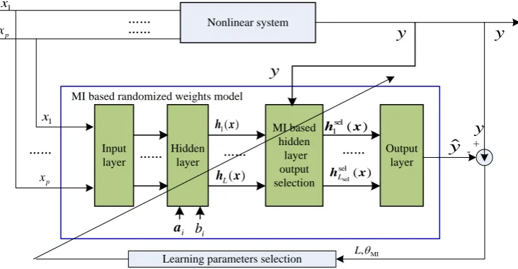
The proposed MI based modified randomized weights neural networks model are shown in Figure 1.

As shown in Figure 1, after obtain the mapping outputs of the hidden layer nodes h x1( ), ∙∙∙ , h xL( ), the MI values between these outputs and predicted variable are calculated with:

(

)

( , )

; ( , ) log ( )

( ) ( ) i

i i i

i

p

MI p d d

p p

=

_∫∫

y h

y h y h h y

h y (18)

Given that pre-set threshold value θMI, the following equation is used to select hidden layer’s outputs:

(

)

(

)

MI

MI

1 if ,

0 else ,

i i i Muin Muin θ ζ θ  _≥  =  <  h y h y h (19)

We denote these hidden layer’s outputs with 1 i

ζ =

h as:

sel sel

sel sel sel

1

[ ( ), , L ( )]k L× =

H h x  h x (20)

where, Lsel is the number of the selected hidden layer’s outputs.

Therefore, Hsel has less randomization than that of the original H. Output weights are also computed us-ing the Moore-Penrose method with:

sel

ˆ_{=( )}+

β H Y (21)

Consideration problem of the learning parameters’ selection, the MI based randomized weights algorithms can be represented as the following optimization problem:

2 2

MI

1 1

min max

min MI max ˆ

Min ( ) ( ( , , ) )

. .

k k

j j j j

j j

E y y k f L y k

L L L

s t

θ

θ θ θ

= =

= − = −

≤ ≤

≤ ≤

∑

∑

β

(22)

Some intelligent optimization methods can be used to address this problem.

5. Application on Modeling Concrete Compressive Strength

Concrete compressive strength data obtained by the experimental studies of the group led by I.C. Yeh in Taiwan

Nonlinear system …… Hidden layer Output layer

y

ˆ

Learning parameters selection

+ -……

……

MI based randomized weights model

y

1 x p x MI based hidden layer output selection …… …… MI ,θ L ) (x hL ) ( sel 1 x h ) ( 1x h ) ( sel sel x hL Input layer ……

[image:4.595.127.493.503.693.2]

1 x p x

y

y

y

i a b_i

Chung Hua University [15]. This dataset contains 1030 samples, each sample has nine columns. The first 7 columns are the input parameters, namely cement, blast furnace slag, fly ash, water, super plasticizer, coarse ag-gregate and fine agag-gregate in concrete per cubic content of the various ingredients of concrete placement. The eighth column is conserved days, and the last column is concrete compressive strength.

Given that L = 300, the MI values between hidden layer’s outputs and predicted variable are shown in Figure 2.

Figure 2 shows that the maximum MI value is almost 10 times than that of the minimum value. Thus, the hidden layer’s outputs are not stability. It is needed to select outputs with high MI values.

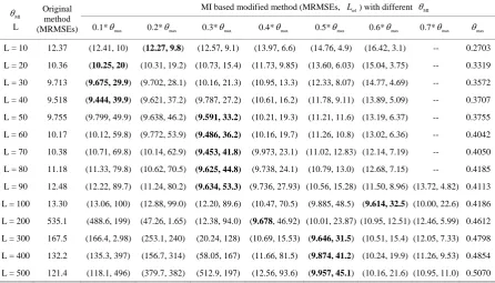
[image:5.595.92.536.244.413.2]

The original randomized weights algorithm and MI based modified version are compared with different hid-den nodes’ number and different MI pre-set threshold values. In order to overcome the randomization of the ini-tial weights, the mean root mean square errors (MRMSEs) with repeated 100 times are used to estimate the model’s prediction accuracy. Statistical results are shown in Table 1.

[image:5.595.90.537.461.716.2]

Figure 2. MI values between hidden layer’s outputs and predicted variable.

Table 1. Statistical results (MRMSEs) of different learning parameters with repeated 100 times.

MI θ

L

Original method (MRMSEs)

MI based modified method (MRMSEs, Lsel) with different θMI

0.1*θmax 0.2*θmax 0.3*θmax 0.4*θmax 0.5*θmax 0.6*θmax 0.7*θmax θmax

L = 10 12.37 (12.41, 10) (12.27, 9.8) (12.57, 9.1) (13.97, 6.6) (14.76, 4.9) (16.42, 3.1) -- 0.2703

L = 20 10.36 (10.25, 20) (10.31, 19.2) (10.73, 15.4) (11.73, 9.85) (13.60, 6.03) (15.04, 3.75) -- 0.3319

L = 30 9.713 (9.675, 29.9) (9.702, 28.1) (10.16, 21.3) (10.95, 13.3) (12.33, 8.07) (14.77, 4.69) -- 0.3572

L = 40 9.518 (9.444, 39.9) (9.621, 37.2) (9.787, 27.2) (10.61, 16.2) (11.78, 9.11) (13.89, 5.09) -- 0.3707

L = 50 9.755 (9.799, 49.9) (9.638, 46.2) (9.591, 33.2) (10.21, 19.3) (11.21, 11.6) (13.19, 6.37) -- 0.3755

L = 60 10.17 (10.12, 59.8) (9.772, 53.9) (9.486, 36.2) (10.16, 19.7) (11.26, 10.8) (13.02, 6.36) -- 0.4042

L = 70 10.38 (10.71, 69.8) (10.14, 62.9) (9.453, 41.8) (9.973, 23.1) (11.02, 12.83) (12.14, 7.19) -- 0.4050

L = 80 11.18 (11.33, 79.8) (10.62, 70.5) (9.625, 44.8) (9.738, 24.1) (10.79, 13.0) (12.68, 7.15) -- 0.4185

L = 90 12.48 (12.22, 89.7) (11.24, 80.2) (9.634, 53.3) (9.736, 27.93) (10.56, 15.28) (11.50, 8.96) (13.72, 4.82) 0.4113

L = 100 13.30 (13.06, 100) (12.88, 99.0) (12.20, 89.6) (10.47, 70.5) (9.885, 48.5) (9.614, 32.5) (10.00, 22.6) 0.4186

L = 200 535.1 (488.6, 199) (47.26, 1.65) (12.38, 94.0) (9.678, 46.92) (10.01, 23.87) (10.95, 12.51) (12.46, 5.99) 0.4612

L = 300 167.5 (166.4, 2.98) (253.1, 240) (20.24, 128) (10.69, 15.53) (9.646, 31.5) (10.51, 15.4) (12.05, 7.33) 0.4798

L = 400 132.2 (135.3, 397) (156.7, 314) (58.05, 167) (11.66, 81.5) (9.874, 41.2) (10.24, 19.9) (11.26, 9.53) 0.4854

L = 500 121.4 (118.1, 496) (379.7, 382) (512.9, 197) (12.56, 93.6) (9.957, 45.1) (10.16, 21.6) (10.95, 11.0) 0.5070

0 50 100 150 200 250 300

0.05 0.1 0.15 0.2 0.25 0.3 0.35 0.4 0.45 0.5

Hidden nodes (n)

Table 1 shows that: 1) The maximum MI values based on different learning parameters between hidden layer’s output and predicted variable increase with the number of the hidden nodes; 2) All smallest prediction errors with different learning parameters (L, θMI) occur with L = 30 - 40; Thus, it may be the best range for this benchmark dataset; 3) The biggest prediction errors occur at about L = 200. The reason may be relate to the Moore-Penrose method; 4) The prediction performance isn’t much improved with the modified approach with L = 40. However, with the other L values, the prediction performance can be improved much with suitable MI pre- set threshold value. Therefore, the largest prediction error problems at L = 200 can be avoided with the MI based modified approach. Thus, the proposed method has better robustness than that of the original randomized weighting algorithm.

6. Conclusion

This paper proposes new mutual information based randomized weights neural networks. Input weights of the hidden layer are produced randomly as normal randomized algorithm. Not all the outputs of the hidden layer are used to compute output weights. Mutual information based simple feature selection method is used to select hidden layer’s outputs. These selected outputs are used to compute weights of hidden layer with pseudo inverse method. Concrete compressive strength benchmark dataset is used to validate this method. More researches will address some theoretically analysis and to validate this idea with more benchmark datasets.

Acknowledgements

The research was sponsored by the post doctoral National Natural Science Foundation of China (2013M532118, 2015T81082), National Natural Science Foundation of China (61573364, 61273177), State Key Laboratory of Synthetical Automation for Process Industries, China National 863 Projects (2015AA043802).

References

[1] Shang, C., Yang, F., Huang, D.X. and Lu, W.X. (2014) Data-Driven Soft Sensor Development Based on Deep Learn-ing. Journal of Process Control, 24, 223-233. http://dx.doi.org/10.1016/j.jprocont.2014.01.012

[2] Pao, Y.H. and Takefuji, Y. (1992) Functional-Link Net Computing, Theory, System Architecture, and Functionalities.

IEEE Computer, 25, 76-79. http://dx.doi.org/10.1109/2.144401

[3] Igelnik, B. and Pao, Y.H. (1995) Stochastic Choice of Basis Functions in Adaptive Function Approximation and the Functional-Link Net. IEEE Trans. Neural Network, 6, 1320-1329. http://dx.doi.org/10.1109/72.471375

[4] Huang, G.B., Chen, L. and Siew, C.K. (2006) Universal Approximation Using Incremental Constructive Feedforward Networks with Random Hidden Nodes. IEEE Transactions on Neural Networks, 17, 879-892.

http://dx.doi.org/10.1109/TNN.2006.875977

[5] Tapson, J. and Schaik, A.V. (2013) Learning the Pseudoinverse Solution to Network Weights. Neural Networks, 45, 94-100. http://dx.doi.org/10.1016/j.neunet.2013.02.008

[6] Alhamdoosh, M. and Wang, D.H. (2014) Fast Decorrelated Neural Network Ensembles with Random Weights. Infor-mation Sciences, 264, 104-117. http://dx.doi.org/10.1016/j.ins.2013.12.016

[7] Bartlett, P.L. (1997) For Valid Generalization, the Size of the Weights Is More Important Than the Size of the Network.

IEEE Conference on Neural Information Processing Systems, MIT Press, Cambridge, 134-140.

[8] Bengio, Y., Lamblin, P., Popovici, D. and Larochelle, H. (2007) Greedy Layer-Wise Training of Deep Networks. Ad-vances in Neural Information Processing Systems, MIT Press, Cambridge, 153-160.

[9] de la Rosa, E. and Yu, W. (2015) Nonlinear System Identification Using Deep Learning and Randomized Algorithms.

IEEE International Conference on Information and Automation (ICIA2015), Lijing, 274-279. http://dx.doi.org/10.1109/ICInfA.2015.7279298

[10] Liu, H.W., Sun, J.G., Liu, L. and Zhang, H.J. (2009) Feature Selection with Dynamic Mutual Information. Pattern Recognition, 42, 1330-1339. http://dx.doi.org/10.1016/j.patcog.2008.10.028

[11] Peng, H.C., Long, F.H. and Ding, C. (2005) Feature Selection Based on Mutual Information: Criteria of Max-Depen- dency, Max-Relevance, and Min-Redundancy. IEEE Transactions on Pattern Analysis and Machine Intelligence, 27, 1226-1238. http://dx.doi.org/10.1109/TPAMI.2005.159

[13] Tang, J., Chai, T.Y., Yu, W. and Zhao, L.J. (2012) Feature Extraction and Selection Based on Vibration Spectrum with Application to Estimate the Load Parameters of Ball Mill in Grinding Process. Control Engineering Practice, 20, 991- 1004. http://dx.doi.org/10.1016/j.conengprac.2012.03.020

[14] Battiti, R. (1994) Using Mutual Information for Selecting Features in Supervised Neural Net Learning. IEEE Transac-tion on Neural Network, 5, 537-550. http://dx.doi.org/10.1109/72.298224