Implementation of RS Encoder and RS Decoder using UHD Architecture

Implementation of RS Encoder and RS Decoder

using UHD Architecture

Naresh.B

M.Tech Student, ECE

Vardhaman College of Engineering, Hyderabad, INDIA

S.Srinivas

Assistant Professor (Sr.), ECE Vardhaman College of Engineering,

Hyderabad, INDIA

ABSTRACT

Reed Solomon (RS) codes are a sort of non-binary cyclic codes. This code is widely used in wireless and mobile communication units. RS encoder along with RS decoder using UHD architecture is designed in this paper. In this brief, a novel low complexity reformulated inverse-free burst-error correction algorithm is developed. Then based on the Proposed RiBC algorithm, a Unified VLSI architecture is designed. It will be shown that, it can achieve high-speed, throughput and improved error correcting capability than Hard Decision Decoding (HDD) design with less area. A design of (7, 3) Reed Solomon encoder and Decoder are implemented using Verilog hardware description language (HDL) code, simulated and synthesized by XILINX ISE simulator.

General Terms

RiBC algorithm,RS codes,UHD.

Keywords

Burst error correction, Hard decision decoding, unified VLSI Architecture

1.

INTRODUCTION

Reed-Solomon (RS) codes are concerned with the detection and correction of errors in symbols. RS codes are widely used for correcting the errors in storage and communication systems [1]. During transmission error may happen for a number of reasons e.g. (scratches on CD, radio frequency interference with mobile phone reception, noise etc.) At the receiving side, the decoder detects and corrects a limited predetermined number of errors occurred during transmission.

When we are dealing with the RS codes as forward error correction, the errors are generated in transmission procedure are divided into burst errors, random errors and erasures[2]. In this brief, a low-complexity high speed RS encoding and decoding architecture will improve the overall system performance significantly. In this a low complexity reformulated inverse free burst-error correcting (RiBC) algorithm is developed for practical applications. Then, based on the proposed reformulated inverse free burst error correcting algorithm, a unified VLSI architecture that is capable of correcting random errors, as well as burst errors and erasures, is firstly presented for multi-mode decoding requirements. It will be shown that, being the first RS Encoder and then decoder owning enhanced burst-error correcting capability, it can achieve significantly better burst error correcting capability than hard-decision decoding (HDD) design.

In this paper, area efficient RS encoder along with RS decoder using UHD architecture are implemented.Section2 discusses the Reed Solomon encoding procedure.Section3 introduces the proposed RiBC algorithm and Section4 covers the proposed unified hybrid decoding Architecture. Experimental results are showing the simulation results of proposed design.

2.

REED SOLOMON ENCODING

2.1

Reed- Solomon codes

Reed-Solomon code is a block code and can be specified as RS (n, k) as shown in Fig1.The variable n is the size of the code word with the unit of symbols, k is the number of data symbols and 2t is the number of parity symbols. Each symbol consists of m number of bits. Reed Solomon codes works on Galois field. The Reed Solomon code allows correct up to t number of symbol errors.Where t is given by

(

) / 2

t



n



k

.

PARITY

DATA

n

k

2t

Fig 1 : The structure of RS Codeword

2.2

Reed-Solomon Encoder

Reed-Solomon codes operate on the information by dividing the message stream into blocks of data, adding redundancy per block, dependent only on the current inputs. The symbols in Reed-Solomon coding are elements of a Galois Field (finite field). Encoding procedure is done by dividing the message polynomial by generator polynomial, then it gives the Galois field remainder. The Galois field remainder is appended to the message[1]. This division is done by a Linear Feedback Shift Register (LFSR) implementation.Reed-Solomon Encoder using LFSR are shown in the Fig 2

.

The Linear Feedback Shift Register is the main computational element of the Reed- Solomon Encoder. The RS encoding procedure is based on Finite Field operations. The generating polynomial for an RS code takes the form

0 1 2 2 2 1 2 1 2 2

( )

....

t t t t

g z

 

g

g z g z



 

g



z





g z

3

( ) 1

Feedback Switch 1

Output symbol sequence

Input message symbol sequence

Switch 2

+ + + +

3





1



0



3

4 Z 3 Z 2 Z 1 Z 0 Z

Fig2: Reed-Solomon Encoder Block Diagram (LFSR)

3.

PROPOSED RIBC ALGORITHM

RS codes are very effective for correcting long burst errors. However, previous decoding algorithms in [5] and [6] are infeasible for hardware implementation due to their high computation complexity, long data path.

3.1

Proposed Reformulated Inverse-free

Burst-Error Correcting (RiBC) Algorithm

In [12] the original burst error correcting algorithm consists of inversion operation and some computational steps contains long data dependency and long data path. To resolve these problems we reformulate BC algorithm to the proposed reformulated inverse free burst error correction algorithm.

The Reformulated inverse free burst error correction algorithm is a kind of list decoding algorithm [4]. In this proposed RiBC algorithm eight polynomials are updated simultaneously in each iteration. After every 2β inner

iterations,

~(2 )

( )

z





, as the candidate of the error locator polynomial of the random errors is computed for current lth outer iteration. When l reaches n, we track the

~(2 )

(z)





, that is identical for longest consecutive l, and record the last element l* of the consecutive l’s. Then the corresponding

(2 )

(z)





and

~(2 )

(z)





, at the l*-th loop are marked as overall error locator polynomial



*

( )

z

and error evaluator polynomial



*

(z)

respectively

Algorithm for Reformulated Inverse - free Burst-Error Correction (RiBC):

f -length ( f<( 2t--2



) burst of errors plus maximum



random errors ):

Input: Syndromes

s s s

_{0, 1}

,

₂

,...

s

_{2 1t} ;

A1: Compute

1 (2 2 ) 2 (2 2 ) 1

(z) (1



 t 

z)(1



 t 

z)...(1





z)(1

z

)

  







2 2 2

1 2 2 2

1



z



z

....



_{t }

z

t 

 







A2: For l=0 step 1 until n-1 do

A2.1: Compute

2 2 2

1 2 2 2

(z)

(



l

z) 1

z

z

...

_t

z

t 

;

  

    

  

A2.2: Compute

2 1

0 1 2 1

(z)

z

...

t

z

t

,

 



    

 

2 2 2 2 0

;

t

i j i t j

j

where

S

 



    

 



A2.3: Initialize

(0) (0) (0) (0) 2 2

0 1 2 2

(z)





z

....



_t

z

t

(z);











 

(0) (0) (0) (0) 2 2

0 1 2 2

(z)

....

_t t

(z);

B



b



b z





b



z



 

~(0) ~(0) ~(0) ~(0)

2 2

0 1 2 2

(z)

...

t

1;

t

z

z























~(0) ~(0) ~(0) ~(0)

2 2

0 1 2 2

(z)

...

t t

1;

B



b



b z





b

_

z





~(0) ~(0) ~(0) ~(0)

2 1

0 1 2 1

(z)





z

...



_t

z

t



(z);













~(0) ~(0) ~(0) ~(0)

2 1

0 1 2 1

(z)





z

...



_t

z

t



(z);













~*(0) ~*(0) ~*(0) ~*(0)

2 1

0 1 2 1

(z)





z

...



_t

z

t

S

(z);













~*(0) ~*(0) ~*(0) ~*(0)

2 1

0 1 2 1

(z)





z

...



_t

z

t

S

(z);













(0) (0)

1,

k

0;







A2.4: For

r



0

Step1 Until

2





1

do

A2.4.1: Compute

~( 1) ~( ) ~( ) ~( )

1 0

;

r r r r

r

i i i







 

_



 

~*( 1) ~*( ) ~( ) ~*( )

1 0

;

r r r r

r

i i i







 

_



 

~( )

1 ( ) ( ) ( )

0 1

;

r

r r r r

i i

b

i





 









~( 1) ~( ) ~( ) ~( ) ( )

0

1;

r r r r

r

i i

bi









 





A2.4.2: If

~( )

0

0

r





and

k

( )r



0

then

a



1

; else

0

a



;

A2.4.3: ( ) ( ) ( 1) 1 ~( ) ~( ) ~( 1) 1 ~( ) ~( ) ~( 1) 1 _ ~*( ) ~*( ) ~*( 1) 1 ~( ) ( ) ( 1) 0

( 1) _{( ) ( )}

1

1

r r r i i i r r r i i i r r r i i i r r r i i i r r r

r _{r r}

b

b

b

b

a

a

k

_k

_k

A3: Track the longest consecutive

~(2 )

(z)





that are identical, recorded the last element

l

* of the consecutive

l s



then the overall error locator polynomial



*

(z)

 

(2 )

(z)

at the

l

*-th outer loop.

The overall evaluator polynomial



*

(z)

is corresponding

~(2 )

(z)





at the

l

*-th outer loop. Output



*

(z)

,



*

(z)

The proposed Reformulated Inverse-free burst error correction algorithm is targeted for correcting burst (local) errors plus some random (global) errors. If the channel condition guarantees that only single long burst of errors occurred. Wu [7] presented a low complexity single long burst of errors correcting (sLBC) for that case. The single long burst of errors correcting algorithm is a special version of Reformulated inverse-free burst error correction algorithm

.

3.2

Algorithm for single long Burst of

Errors Correction (sLBC)

Input: Syndromes

s s s

_{0, 1}

,

₂

,...

s

_{2 1t} ; B1: Compute

1 (2 1) 2 (2 1)

(z)

(1



 t

z)(1



 t

z)....(1

z

)



 





2 2 1

1 2 2 1

1



z



z

....



t

z

t

 

 







B2: Compute

2

2 2 1

2 1 2 2 1 2 3 0 2 1

(z)

s

_t

s

_t



z

s

_t



z

....

s



_t

z

t











B3: B3.1: Find roots of



(z)

;

B3.2: Track the longest consecutive root sequence

1

s





,



s,…..



s 2t 2 ;

B3.3: Use t to calculate the value of s,



,

Then it can claim that a burst of errors starts at position



s with length



;

B4: Compute new error locator polynomial

* 2 2

(z)

(



s t

z)



 

B5: Compute new error value polynomial

* 2 1

0 1 2 1

(z)

...

t

t

z

z

 

















Where



_i

 

*₀

s

_i

 

*₁

s

_i1



...

 

*_i

s

₀

for

i



0,1, 2...2

t



1

;

Output



*

(z)

,



*

(z)

3.3

Algorithm for Random Error and

Erasure Correction (rEEC)

Input: Syndromes

s s s

_{0, 1}

,

₂

,...

s

_{2 1t} ;

Erasure locations:

z z

₀

,

_1,

...,

z

_1

;

 

2

t



2

C1: Compute

0 1 1

(z)

(1 z z)(1

z

z)....(1

z

_

z)



 





2

1 2

1



z



z

...



_

z



 







C2: Compute

2 1

0 1 2 1

(z)

z

....

_t

z

t



    

 

where

0

i j i j

j

s





 

 



;

C3: Initialization:

(0) (0)

(z)

B

(z)

(z)





 

(0) (0) (0) 0 2 1

0 1 2 1

(z)





z

....



_t

z

t

(z)











 

(0) (0) 0 0 2 1

0 1 2 1

(z)





....



_t

z

t

(z)











 

(0) (0)

k



0,





1

C4: For r=0 step 1 until

2

t

  

1

do C4.1: Compute

( 1) 1 (r) (r) (r) (r)

0

(z)

x

(z)

(z)

r 















;

( 1) (r) (r) (r) (r)

0 0

(z)

(z)

x

(z)

x

(z)

r r

B



















C4.2: If



₀( )r



0

and

k

(r)



0

then a=1; else a=0;

(r) (r)

( 1)

1 (r) ( )

(r 1)

(r)

(r 1) (r)

0

( 1) (r) (r)

(z)

(z)

(z)

(z)

(z)

1

1

r

r

r

xB

B

a

x

a

k

k

k









 

 





















_{ }







_

_



_{ }

_{ }









_{ }

 

























 



Output:,



*

(z)

 

(2t)

(z)

4.

UHD ARCHITECTURE

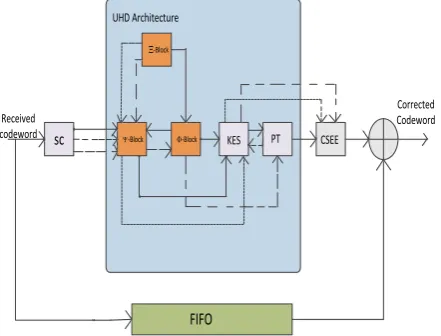
The above three algorithms are share many similar computation steps. Based on this interesting similarity, a UHD architecture is designed. Figure 3 shows the overall architecture of Unified Hybrid Decoding decoder. Three types of lines illustrate data flows for different work modes: solid line for mode-1 for burst combined with random error correction RiBC algorithm, dashed line for mode-2 for only burst error correction and big dashed line for mode-3 for only random error correction. Different blocks are used to process different steps in algorithm.

sc

Received codeword

FIFO

KES PT CSEE

Corrected Codeword UHD Architecture

-Block



-Block

[image:3.595.317.538.552.720.2]

 -Block

A Reed–Solomon decoder consists of mainly four blocks:

 The syndrome computation (SC) block.

 The key Equation solver (KES) block.

 Position tracking (PT) block.

 The Chien search and error evaluator (CSEE) block

4.1 Syndrome Calculation

The first step in decoding process is the received symbol is to determine the data syndrome.The syndrome calculation block is used to check whether the received polynomial contains errors or not. The syndrome generation block evaluates the received codeword polynomial. If the received codeword consists an error then the syndrome polynomial is non zero.If received codeword contains an error, it indicates that the received syndrome polynomial is zero,and the data is passed through the decoder without any error correction.The syndromes can then be calculated by substituting the 2t roots of the generator polynomial G(z) into R(z). The syndrome polynomial is generally represented as, Where α is the primitive element.

1 0

(

)

n i ij i j j

S

r



r













,

i



0,1,....(2

t



1)

4.1.1

Block :

- block is used to carryout steps A1, B1, or C1 in different work modes. No matter which work mode is selected, the computation of (z) is always carried out as follows

:

2

1 1 2

( )

z

_i_

(1

A z

_i

) 1



( )

z



z

...



_

z



  



 







Where denotes or , and



denotes 2t-2 , 2t-1.

4.1.2

Block:



block used to process Steps A2.1 and B3.1. For these steps, the common operation is multiply accumulate for each coefficient of the polynomial. Only a slight difference exists in step B3.1 it is a Chien Search-like step, hence an extra adder tree is required to verify the validity of current received

symbol. For each

l

in step A2.1 since

2 2

1 2

[ ]

z

(



l

z

)

1



z

...



_t

z

t 



 

 





should be maintained within 2t+3 cycles

4.1.3

Block:

-block is used to process steps A2.2, B2 and C2. Actually, the inherent nature of steps A2.2, B2 and C2 is the multiplication of two polynomials

.

4.2

Key Equation Solver Block

Architecture

This is the heart of the Reed-Solomon Decoder. This KES block generates the Error Locator polynomial



(z)

. After the Error Locator polynomial has been found, it is used to determine the Error Evaluator polynomial



(z)

.

In this step with the help of S(z), KES block will calculate error locator polynomial Λ(z) and error evaluator polynomial

(z)



by solving key equation: Λ(z)S(z)=



(z)

mod

z

2t.

Key equation solver block determines the overall system performance significantly.The overall decoding process is done by using this key equation solver only.

Control

PE 10 PE 11 PE 12t-2 PE 12t-1

PE 02t-2 PE 02t-3 PE 01 PE 00

ctrl

0 0

0 0

( )r 

( )r



( )r

[image:4.595.320.535.111.284.2]

 ( ) 0 r  ( ) 0 r  ( ) 0 r 

Fig 4:Overall architecture of Key Equation Solver block

In UHD decoder KES block is carry out steps A2.4, B4, B5 and C4. Fig 4 represents the overall architecture of KES block and internal structures of its two types of processing elements (PE): PE0 and PE1 are shown in the Fig 5 and Fig 6. As shown in fig 4 the KES block consist of 2t-1PE0’s and 2t PE1’s in the rth

iteration. Each register in PE0i / PE1i stores the corresponding coefficients of different polynomials(Fig5, Fig6). D D D D 1 1 1 0 0 0

Group A Ctrl 1

ctrl ( )r



(r) 0



( )r i

b

( )r i b (r) i  (r) i  1 i 

( )r



( r ) 0



(r) 1 bi

(r) 1 i

b

Fig 5: Block diagram of

PE

0

_i

D D D D 1 1 0 0 ctrl

( )r  (r) 0  (r) 0  Group B Group C

( )r i



( )r i 

( ) *r

i  *( )ir

(r)

i 

( r ) *

i 

( )r

[image:4.595.327.530.389.752.2]

 ( ) 1 r i   ( ) * 1 r i  

4.3

Position Track (PT) Block

PT block is used to track the longest consecutive polynomials that are identical or positions of roots that is steps B3.2 and B3.3.

The inputted from KES block at the lth

outer iteration are denoted as

~

( )

i

l



, and

~

( )

i

l



. In

addition, ) (temp) represents

~

(

1)

i

l





, while

~

( )

i

l



(store) are the coefficients of current continuously identical . Moreover, (longest) stores the coefficients of current longest continuously identical

_{. Control signals shift and equalare generated from}

signal generation Schedule. After l reaches n, (longest) and

~

i



(longest) are outputted as the coefficients of overall error locator polynomial and overall error evaluator polynomial



*

( )

z

.

4.4

Chien Search and Error Correction

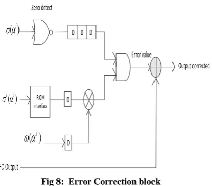
In this approach error locator polynomial and error value polynomial values are passed to the Chien search and Forney algorithm blocks. To find the error location, Chien search is the very good efficient method. Chien search method is used for finding error positions. Fig7 shows the basic Chien search block. Error correction block is shown in the Fig8.Its basic

idea is simple but efficient: If



(



i

)



0

for current i, it indicates that the ith symbol of the received codeword is wrong and needs to be corrected. After obtaining the error positions, the following Forney algorithm is applied to determine the error value.

1

1

(X )

(

)

i i

i

X



 



 



whereYi indicates error magnitude for the ith erroneous

symbol.

Cx ₀

1

D Ci

[image:5.595.330.537.77.258.2]

α l

Fig 7: Basic Chien search cell

Zero detect

FIFO Output

ROM interface

D D D

D

Error value

Output corrected

( )

i

 

( )

i

 

( )

l i

 

D

Fig 8: Error Correction block

[image:5.595.319.541.363.498.2]

The block diagram of proposed architecture is shown in the Fig9. The encoded output being given to the decoder along with introduction of noise. The decoder is fed with all the information need for decoding after a certain latency it will check whether all the code words are valid code words, if so it will output or else it will correct them, if the number of corrupted code words are less than the maximum error correcting capability of the RS Decoder.

Fig 9: Block Diagram of Proposed Architecture

5.

EXPERIMENTAL RESULTS

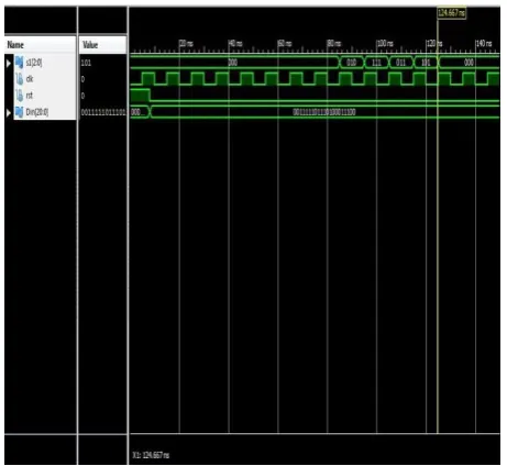
The Simulation results of proposed architecture are carried out using Xilinx ISE simulator.

[image:5.595.58.271.495.660.2]

Fig11: Simulation result for Syndrome

Fig12: Simulation result for decoder

Fig13: Simulation result for Encoder _Decoder

[image:6.595.52.283.70.282.2]

Fig14: Simulation result for Encoder_ Decoder

Fig 15: Final output for proposed Architecture

Message will be passing from encoder to decoder.The decoder checks the resulted data and gives the error free data. Fig15 shows the output of proposed architecture.

6.

CONCLUSION

7.

REFERENCES

[1] B.Sklar, “ Digital Communication, Fundamental and Application” Prentice Hall, Upper Saddle River, 2001.p.1104.

[2] S.B.Wicker and V.K. Bhargava, eds “Reed-Solomon codes and their applications” New york: IEEE press 1994.

[3] Amina, P. Chio, I.A. Sahagun and D. J. Sabido IX “VLSI Implementation of A (255,223) Reed- Solomon Error- Correction Codec,” Roc. Of Second National ECE Conference.

[4] D.V. Sarwate and N.Rshanbhag, “High-speed Architectures for Reed-Solomon Decoder,” IEEE transaction on VLSI system, OCT, 2001.

[5] E. Dawson and A. Khodkar, “Burst error-correcting algorithm for Reed-Solomon codes,” Electron. Lott, vol. 31, pp. 848–849, 1995.

[6] L.Yin, J.Lu, K.B.Letaief and Y.Wu Burst-error-correcting algorithm for Reed-Solomon codes.

Electronics Letters.,vol. 37, no. 11, pp.695-697, may 2001.

[7] Y. Wu, “Novel burst error correcting algorithms for Reed-Solomon codes,” in Proc. IEEE Allerton Conf. Commun., Control, Comput.2009, pp. 1047–1052.

[8] R. E. Blahut, Theory and Practice of Error-Control Codes. Reading, MA: Addison-Wesley, 1983.

[9] H.C.Chang and C. B. Shung, , “New serial architectures for the Berlekamp–Massey algorithm,”IEEE Trans. Commun. vol. 47, pp. 481–483, Apr. 1999.

[10]K. Bhargava, Eds. Piscataway, NJ: IEEE Press, 1994. Algorithms and architectures for a VLSI Reed– Solomon codec.

[11]T. Zhang and K. K. Parhi, “On the high-speed VLSI implementation of errors-and-erasures correcting Reed-Solomon decoders,” in Proc. ACMGreat Lake SympVLSI (GLVLSI), 2002.