Improving Fault Prediction using ANN PSO in Object Oriented Systems

(1)

Improving Fault Prediction using ANN-PSO in Object

Oriented Systems

Kayarvizhy N

Associate Professor, Department of Computer Science and Engineering, AMC Engineering College Bangalore – 560076, India

Kanmani S

Professor, Department of

Information Technology, Pondicherry Engineering College, Puducherry – 605014,

India

Rhymend Uthariaraj V

Professor & Director, Ramanujam Computing Centre Anna University, Chennai, India

ABSTRACT

Object oriented software metrics are computed and used in predicting software quality attributes of object oriented systems. Mapping software metrics to software quality attributes like fault prediction is a complex process and requires extensive computations. Many models have been proposed for fault prediction. Since accuracy is of prime importance in prediction models they are being constantly improved through various research studies. Artificial Neural network (ANN) has gained immense popularity due to its adaptability to the problem at hand by training with known data. Back propagation is a widely used ANN training technique. However the back propagation technique leads to slow convergence rate and an impending threat of getting caught in local minima. In this paper we explore the Particle Swarm Optimization (PSO) technique as an alternative to optimize the weights of ANN for fault prediction in object oriented systems. We evaluate the effect on prediction accuracy that PSO brings to ANN compared to other techniques like BP and Genetic Algorithm (GA). We also evaluate prediction accuracy improvements by optimizing the various parameters of PSO.

General Terms

Software Quality, Object Oriented Metrics and Particle Swarm Optimization.

Keywords

swarm intelligence, particle swarm optimization, object oriented metrics, artificial intelligence, software quality.

1. INTRODUCTION

Software quality is the most sought after aspect of an object oriented software system during and after its development. Software quality could be affected by a variety of factors and occurrence of faults negatively impacts quality. Early detection and removal of faults from the system is a major step towards good quality software. Bellini et al [1] compared the different models of fault prediction and concluded that software quality has become one of the most important requirements of a software system and that fault prediction could be the key in controlling the quality of software systems. Early prediction of the modules that could potentially have a large number of faults saves a lot of effort, time and cost and allows a focused approach for quality enhancement measures.

A software quality model attempts to map an external quality attribute (in this case faults) of software to its internal attributes like size, inheritance, coupling, and cohesion. When the internal attributes are measured and assigned a value; they are referred as software metrics. Once the quality attributes (external) are predicted using the software metrics (internal), it becomes easy to control the quality of the product. During the development of a software product the internal attributes are measured and fed to the model. Based on the prediction made by the model for the quality indicator, necessary corrective and preventive actions can be taken. This ensures that quality is managed even during the design and development stage of a software product. Many software quality prediction models have been proposed in the literature [2] [3] [4] [5] [6] [7] [8]

Prediction accuracy is an important criterion that differentiates software quality prediction models, the better the prediction accuracy the more useful its application. Hence strong emphasis is placed on improving the prediction accuracy of models. So research efforts are focused not only on proposing newer prediction models but also on improving the prediction accuracy of existing, already proposed models. Artificial neural network (ANN) is a non-linear mapping model, representing the functioning of a human brain. ANN is a powerful tool for modeling and have been successfully applied to many areas like bankruptcy prediction [9] [10] [11], handwriting recognition [12] [13], product inspection [14] [15], and in fault detection [16] [17]. ANN is also a widely accepted choice of fault prediction model [18] [19] [20] [21]. ANN is adaptive as it can change its structure based on the information that flows through the network. This adaptability is achieved by training the ANN with known data set. In an ANN based prediction model, prediction accuracy can be improved by optimizing the parameters of the model. ANN parameters like number of input neurons, hidden layers, hidden neurons, activation function, weights, etc can be optimized. Since weights are the key to a well trained ANN, which can map the inputs to outputs accurately, optimizing weights of ANN has been considered in many research studies.

(2)

confirmed that back propagation is prone to the following problems – it may get stuck at a local optimum [22] and it may take a very long time to converge [23]. This led researchers to attack the ANN training problem with other methods.

Another technique for ANN weight optimization is by using Genetic algorithms (GA). GA introduced in 1970s by John Holland, are a family of evolutionary computation models inspired by the concepts of genetics and evolution. GA encodes the ANN weights as possible solutions for the problem in the chromosomes of simulated biological organisms. In each generation the organisms with best chromosomes are chosen for reproduction. The probability of crossover and mutation can be adjusted to determine the outcome of the final result. This continues for a predefined number of generations or until the problem is sufficiently optimized. GA has parallel search strategy and global optimization characteristics which helps the ANN to have a higher prediction accuracy and faster convergence compared to BP [24]. However the genetic operators like crossover and mutation are inherently complex and hence make the computational cost to increase exponentially [25]. The convergence speed of GA, though better than BP, is still slow and even stagnates as it approaches the optimum [26]. In this paper our focus would be on ANN weight optimization using Particle Swarm Optimization (PSO), PSO like GA, is an evolutionary computation technique developed by Russel Eberhart and Kennedy in 1995 [27] inspired by social behavior of a flock of birds or school of fish. In PSO, potential solutions like the weights of ANN are considered as particles moving in the problem space. Iteratively, the particles learn from each other and arrive at the optimal solution for a given problem. PSO algorithm is used in many applications involving prediction and forecasting like prediction of chaotic systems [28], electric load forecasting in [29], time series prediction [30] and stock market decision making in [31] [32]. PSO is known to have a strong ability in training ANN [33] [34] [35] for fault prediction. Unlike GA, PSO has no evolution operators such as crossover and mutation. Another advantage that PSO has over GA is that there is no special requirement of encoding and decoding operators for training the neural network.

The aim of our research is to have ANN trained by PSO technique and observe the changes to prediction accuracy. We compare the prediction accuracy of ANN-PSO with the prediction accuracy of ANN models trained by BP and GA techniques. We also explore optimizing the various parameters of the PSO algorithm and how such optimization affects the ANN-PSO prediction accuracy. For these experiments we have considered data sets available online. In section 2 we describe the Artificial Neural Network (ANN) and its training mechanism. In Section 3 we introduce Particle Swarm Optimization (PSO) algorithm and the steps involved in it. We then introduce the ANN-PSO model where the optimization of weights of ANN is done by the PSO algorithm. Section 4 describes the experimental setups with ANN-BP, ANN-GA and ANN-PSO and the comparative results for them. Further experiments which consider the various PSO parameters and the resulting optimum parameters values are also shown in Section 4. Section 5 provides the conclusions and future course of actions derived from this study.

2. FAULT PREDICTION USING ANN

2.1 Artificial Neural Network

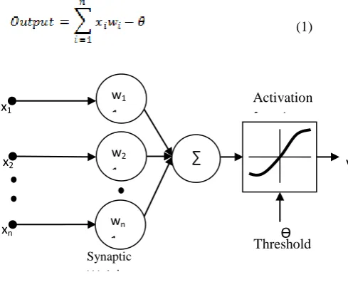
Artificial Neural Network (ANN) is a simplified model of the human nervous system. It is composed of many artificial neurons that co-operate to perform the desired functionality. ANN is an approximation function mapping inputs to outputs. The ability to learn and adapt to the data set makes ANN applicable in a variety of fields. A single neuron in ANN, shown in Figure 1, takes its weighed inputs and produces a single output as given by formula (1).

(1)

[image:2.595.317.562.191.389.2]

Fig 1: Artificial Neuron

The artificial neurons can be combined to form an artificial neural network. A typical artificial neural network has three layers – input, hidden and output. There are „n‟ input neurons to map the inputs and „m' hidden neurons in a single hidden layer. There could be more than one hidden layer as well. The output neurons depend on the number of output variables that we plan to map. Weights are used between input and hidden and hidden and output layers respectively.

ANN exhibits some remarkable properties like adaptability, learning by examples and generalization which makes it an ideal candidate for pattern classification problems. Fault prediction is a subset of classification problem where the fault prone modules need to be identified and tagged. In the case of object oriented systems the lowest level of abstraction is a class. The prediction models like ANN identify classes that could be faulty and tag them. The development team can then work on the tagged classes and design them better.

The first step in the creation of a good fault prediction model based on ANN, involves providing known information with which the model can be trained. In our case we need to have class level metrics data along with the fault details. The ANN model is trained using this information. Once trained the ANN model is ready to be used on fresh data set where only the metrics are known and fault has to be predicted. The ANN model is used to predict whether the classes in the fresh data set are likely to be faulty or not. A properly trained ANN would have a higher probability of prediction the faultiness of classes. The probability is captured by the prediction accuracy which is the percentage of correct classifications compared to the overall classification. Though the prediction accuracy of an ANN fault prediction model depends on various factors like dataset, domain etc, the selection of good ANN parameters is a major contributor.

w1

11

∑

x1

x2

xn

Synaptic

Weights

Activation

function

y

ϴ

Threshold

w2

11

wn

(3)

2.2 ANN Parameter Optimization

ANN is a complex model and its prediction accuracy can be improved by optimizing its parameters. The parameters that can be optimized in an ANN can be grouped under the following categories

 Architecture

o Number of input neurons

o Number of hidden layers and hidden neurons

o Number of output neurons

 Training

o Weights

o Training algorithm o Training epochs

 Transfer function

 Data

o Selection o Pre-processing o Quantity and quality

The major challenge in constructing an ANN model is to find the right values for all these parameters. Among these parameters, weight optimization is considered an important criterion that affects the performance of an ANN. ANN has to be trained to get the optimal values for the weights. The method employed is to have known samples of data with both independent and dependent variables and alter the weights based on how well the ANN predicts the dependent variable (output) for given independent variables (inputs). The difference in the values between predicted and actual is the error. The aim is to minimize this error. This training can be done in a variety of ways like gradient descent, GA, PSO, Fuzzy Logic etc.

The training of an ANN is independent of the ANN structure and hence can be decoupled and worked on separately. For example, the same ANN, could be trained using different algorithms like BP, GA, Fuzzy etc and we could then compare how each of the training algorithm fared in predicting the faults. This would help us to narrow down on the best training algorithm for ANN with the given data set.

3. TRAINING ANN USING PSO

3.1 PSO

PSO employs social learning concept to problem solving. It was developed by James Kennedy and Russell Eberhart in 1995. This is an evolutionary computation method based on the intelligence gained by a swarm through co-operation and sharing of information. Birds flocking together generally exchange valuable information on the location of the food. When a bird learns of a promising location, its experience grows about the surrounding. This is hugely enhanced when the birds share the information with one another, boosting the swarm‟s intelligence. This helps other birds to converge on the most promising food location. PSO is widely applied in many research areas and real world applications as a powerful optimization technique. Simulating the natural behavior, the PSO algorithm has a set of particles that fly around an n-dimensional problem space in search of an optimal solution.

To start with, the particles are distributed randomly in the solution space. Each particle P in the swarm S is represented as {X, V} where X = {x1, x2, x3… xn} represents the position of the particle and V = {v1, v2, v3… vn} represents the velocity of the particle. In every iteration, the particles learn from each other and update their knowledge regarding the whereabouts of a good solution. Each particle keeps track of its best solution with its corresponding position in pbest and the swarm‟s best position is tracked in gbest. Each particle will have the influence of its current direction shown in dotted arrows, the influence of its memory (particle‟s local best - pbest) shown as plain arrows and the influence of the swarm‟s intelligence (global best – gbest).

The particles update their velocity and position based on the formula given in Equation (2). Here „i‟ represents the particle number, „d‟ represents the dimension, „V‟ is the velocity, „p‟ is the pbest, „g‟ represents gbest, „w‟ is the inertia weight, c1 and c2 are the constants for controlling the influence of pi and g respectively, „x‟ is the current position and „rp‟ and „rg‟ are random numbers between 0 and 1.

(2)

Pseudo code of PSO algorithm

1. For each particle i = 1, ..., S do:

a. Initialize the particle's position with a uniformly distributed random vector: xi with

values between the lower and upper boundaries of the search-space.

b. Initialize the particle's pbest to its initial position: pi ← xi

c. If (Objf(pi) < Objf(g)) update the swarm's best

known position: g ← pi

d. Initialize the particle's velocity vi randomly

between the min and max velocity

2. Until a termination criterion is met (Total iterations reached or adequate objective function value is found), repeat:

a. For each particle i = 1, ..., S do:

i. For each dimension d = 1, ..., n do: 1. Pick random numbers: rp,

rg between 0 and 1

2. Update the particle's velocity using equation (2) ii. Update the position: xi ← xi + vi

iii. If (Objf(xi) < Objf(pi)) do:

1. Update the particle's best known position: pi ← xi

2. If (Objf(pi) < Objf(g))

update the swarm's best known position: g ← pi

3. Now g holds the best found solution.

PSO is simple to implement with less number of parameters to adjust. PSO has been used successfully in function optimization, neural network training and many more fields requiring optimization

3.2 ANN-PSO

(4)

number of weights that needs to be optimized. Each particle has a position vector and a velocity vector of n-dimensions. The PSO particles fly around this search space and come up with the optimal set of weights. While evaluating the fitness of a particle in PSO, the weights are assigned to the ANN and its prediction accuracy is found. This provides the fitness for the particle. If the fitness is the best so far for the particle it will be taken as its personal best and if it is the best so far for the swarm, it would be considered as global best. The global best position after a desired number of iterations yield the optimized weights for the ANN. The steps for a PSO optimized ANN is given below.

Pseudo code of ANN-PSO algorithm

Define the ANN architecture – number of input, hidden and output neurons.

Identify the fitness function which returns the error as difference of actual and predicted output for the ANN Initiate a swarm of ‘x’ particles with random weights of ‘n’ dimension where n is the total number of weights that needs to be optimized for the ANN

For each iteration do this to the x particles

Find the fitness of each particle as defined in Step 2 Update pbest if the fitness is better than pbest Update gbest if the fitness is better than gbest Update velocity and position

Do the steps till the iterations are completed

gbest has the best weights for the ANN which yields the highest prediction accuracy.

4. EXPERIMENT AND ANALYSIS

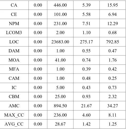
[image:4.595.311.550.71.315.2]

We conducted two kinds of experiments. The first experiment was to compare the prediction accuracy of ANN-PSO against other ANN optimization techniques like Back propagation (ANN-BP) and Genetic Algorithm (ANN-GA). The second experiment was to explore various values for the ANN-PSO parameters and see their effect in prediction accuracy. To conduct these experiments we used six projects from the Promise data set [37] including different versions of the projects resulting in a total of 7773 samples. Each data set sample consisted of twenty object oriented metric values and their corresponding bug data. Table 1 gives the snapshot of the metric values – minimum, maximum, mean and standard deviation. The list of metrics is described in Appendix A.

Table 1. Snapshot of the Metric Values

Metric Min Max Mean SD

WMC 0.00 413.00 10.21 17.61

DIT 0.00 8.00 2.12 1.47

NOC 0.00 52.00 0.47 2.46

CBO 0.00 448.00 10.68 17.53

RFC 0.00 583.00 28.66 39.30

LCOM 0.00 41713.00 117.16 1017.58

CA 0.00 446.00 5.39 15.95

CE 0.00 101.00 5.58 6.94

NPM 0.00 231.00 7.51 12.29

LCOM3 0.00 2.00 1.10 0.68

LOC 0.00 23683.00 275.17 792.85

DAM 0.00 1.00 0.55 0.47

MOA 0.00 41.00 0.74 1.76

MFA 0.00 1.00 0.39 0.42

CAM 0.00 1.00 0.48 0.25

IC 0.00 5.00 0.43 0.73

CBM 0.00 25.00 0.93 2.32

AMC 0.00 894.50 21.67 34.27

MAX_CC 0.00 236.00 4.60 8.11

AVG_CC 0.00 28.67 1.42 1.25

4.1 Comparison of ANN Models

Three different prediction models were constructed for this experiment, one each for ANN-BP, ANN-GA and ANN-PSO. In all the models 70% of the data was used for training and 30% for validation. Each data set was submitted five times to the models and the average prediction accuracy was computed. This was done to avoid any bias resulting from a skewed single run. ANN-BP model was constructed in Matlab using the Neural Network Toolbox. For the ANN architecture we chose 20 input neurons, one hidden layer with 25 neurons and one output neuron. The input neuron number was chosen to match the number of metrics and the output was chosen to match the bug data results. The training was done for a hundred epochs using BP and gradient descent. The hidden neurons and epochs were based on the earlier experimental attempts by other researchers. This number was probed further in the second set of experiments that we had conducted. The ANN-GA prediction model was done using a tool taken from an open source code project [38] and modifying it as required. The tool was originally developed to help in a facial recognition model. The tool also had a requirement that the data set given as input needs to be split as buggy and bug-free samples, we wrote a simple script to partition the data set before submitting it to the ANN-GA tool. The GA parameters were adjusted as given in Table 2 based on recent research in GA.

Table 2. Control Parameters for GA in ANN-GA

Parameter Value

Number of Population 20

Number of Generation 200

Crossover Probability 0.50

Mutation Probability 0.001

Selection function Roulette Wheel

Fitness Prediction accuracy

(5)

The ANN-PSO algorithm was developed as a tool in Visual Studio by the authors to aid in this study. The tool takes in the metrics and bug information from a comma separated data file and computes the prediction accuracy. The tool randomizes the data before making the 70%-30% split for training and validation.

Table 3 provides the control parameters used for running PSO in the ANN-PSO model. These parameters were taken from earlier PSO research experiments and have been optimized our second set of experiments.

Table 3. Control Parameters for PSO in ANN-PSO

Number of Particles 20

Number of Iterations 100

Inertia Weight 0.529

Local Weight (c1) 1.4944

Fitness Prediction accuracy

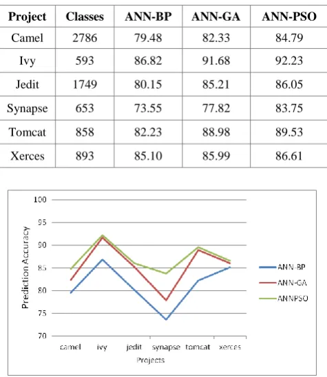
[image:5.595.49.287.440.714.2]

Table 4 and Figure 2 provide the prediction accuracy values for the various experimental setups. We find that ANN-GA predicts compared to ANN-BP by an average of 4.11%. The prediction accuracy of ANN-PSO is better compared to the prediction accuracy of ANN-BP by 5.94% and marginally better compared to the prediction accuracy of ANN-GA by 1.82%. Also for every dataset ANN-PSO predicts better than the corresponding ANN-GA and ANN-BP models.

Table 4. Prediction accuracy of ANN models

Project Classes ANN-BP ANN-GA ANN-PSO

Camel 2786 79.48 82.33 84.79

Ivy 593 86.82 91.68 92.23

Jedit 1749 80.15 85.21 86.05

Synapse 653 73.55 77.82 83.75

Tomcat 858 82.23 88.98 89.53

Xerces 893 85.10 85.99 86.61

Fig 2: Comparison of ANN Training Algorithms

4.2 PSO Parameter Optimization

The second set of experiments that we carried out was to optimize the various parameters of ANN-PSO and identify values for those parameters which resulted in maximum prediction accuracy. The following parameters were considered for optimization

 Number of Particles

 Number of Iterations

 Inertia weight

 Weights for global and local bests

 Number of hidden neurons

4.2.1 Number of Particles

The number of particles in ANN-PSO signifies the amount of area that could be covered in the problem space, in every iteration of the loop. We investigated the ANN-PSO with 5, 10, 20, 50, 75 and 100 particles. ANN-PSO was not able to perform well at 5 and 10 particles since the space covered in the problem is not sufficient. As the number of particles increased to 20 and 50, the prediction accuracy improved. However once the number reached 50, further increase did not result in improvement. In fact with 100 particles we saw a fall in the prediction accuracy as there could have been an over fit of the data. Also the optimization time was getting longer as the number of particles was increased. This is because the optimization time is directly dependent on the solution space covered and with more particles we had to cover more of the space at the expense of time.

[image:5.595.309.549.469.746.2]

Table 5 shows the performance of ANN-PSO with the different number of particles considered. Figure 3 shows the prediction accuracy mapped for the various numbers of particles.

Table 5. Optimization of Particle number

Particles Accuracy

5 82.16

10 85.35

20 89.80

50 90.44

75 90.44

100 73.44

(6)

4.2.2 Number of Iterations

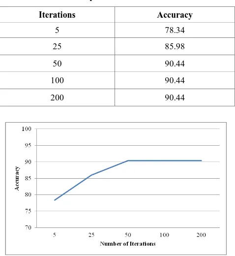
[image:6.595.311.549.82.341.2]

ANN-PSO is investigated with 5, 25, 50, 100 and 200 numbers of total iterations. Table 6 compares the effect that the various values had on prediction accuracy. As the number of iterations increases more of the problem space gets covered and hence the accuracy improves. At 5 and 25 iterations the ANN-PSO is under trained and unable to approximate the underlying function of metrics to faults. After the iterations reached 50, the prediction accuracy did not improve any further, but the time taken for optimization kept on increasing with increase to the iterations. Figure 4 captures these findings.

Table 6. Optimization of Iterations

Iterations Accuracy

5 78.34

25 85.98

50 90.44

100 90.44

200 90.44

Fig 4: Number of iterations affecting Accuracy

4.2.3 Different c1 and c2 values

The constants c1 and c2 are the accelerations constants that pull the particle towards its global or personal best. The c1 indicates the influence that the global best has on the particle and c2 indicates the level of influence that the personal best has on the particle. Reasonable results were obtained when the values of c1 and c2 were ranging between 1.2 and 1.7. With the value of 1.0 the acceleration was not enough to cover the problem space well and resulted in poorer prediction accuracy. There was again a mild drop in prediction accuracy when the acceleration constants reached 2.0. Table 7 gives the prediction values for the various values of c1 and c2. Figure 5 provides the same information as a graph between prediction accuracy and c1/c2 values.

Table 7. Optimization of c1 and c2 values

c1/c2 Accuracy

1.0 70.56

1.2 88.53

1.5 90.44

1.7 90.44

2.0 89.80

Fig 5: c1/c2 values affecting Accuracy

4.2.4 Number of hidden neurons

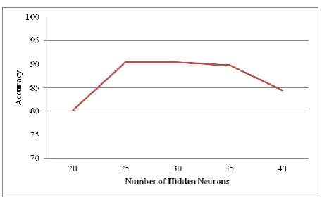
The PSO-ANN was investigated with 20, 25, 30, 35 and 40 hidden neurons in the hidden layer of the architecture. This is not a PSO parameter but a parameter of the ANN architecture in the ANN-PSO model. Table 6 presents the results of this study. At a low value of 20 hidden neurons, the network does not have sufficient flexibility to learn and adapt to the data. This results in low prediction accuracy. Similarly for hidden neurons greater than 30, the ANN taken a long time to get trained and may also be over fitting the data. So the optimum number of hidden neurons was found to be between 25 and 30. The results are captured in Table 8 and Figure 6.

Table 8. Optimization of hidden neurons

Neurons Accuracy

20 80.17

25 90.44

30 90.44

35 89.80

[image:6.595.49.288.214.474.2]

(7)

Fig 6: Number of hidden neurons affecting Accuracy

4.2.5 Optimal Configuration for ANN-PSO

[image:7.595.53.282.67.211.2]

The optimal configuration for ANN-PSO network was found to be as given in Table 9.

Table 9. Optimum configuration values for ANN-PSO

Number of Particles 25

Number of Iteration 50

Hidden Neurons 25 to 30

5. CONCLUSIONS

We explored the particle swarm optimized technique as a training algorithm for artificial neural network (ANN-PSO) to predict the fault proneness of object oriented systems. We found that compared to BP and GA, PSO was able to improve the fault prediction accuracy and speed up the convergence simultaneously. The experimental results conducted on six data sets from promise data repository revealed that PSO is a promising training algorithm for fault prediction in OO systems using OO metrics and its potential should be explored further in this area.

We also experimented with different values for the ANN-PSO configuration parameters. We were able to conclude on the values for configuring the ANN-PSO model to give the best possible prediction accuracy. Future studies could include optimizing more than one parameter of ANN using simultaneous optimization techniques like co-operative PSO and multi objective PSO. Studies can also be done where empirical analysis is done on a wide variety of data set especially industrial projects.

6. REFERENCES

[1] Bellini P. (2005), “Comparing Fault-Proneness Estimation Models”, 10th IEEE International Conference on Engineering of Complex Computer Systems (ICECCS'05), China, pp. 205-214.

[2] Khosgoftaar TM, Gao K, Szabo RM (2001) An Application of zero-inflated poisson regression for software fault prediction, Proceedings of 12th international symposium on software reliability engineering, pp:63-73

[3] Eman K, Benlarbi S, Goel N, Rai S (2001). Comparing case-based reasoning classifiers for predicting high risk

software components. Journal of System software 55(3):301-310

[4] Khosgoftaar TM, Seliya N (2002). Tree-based software quality estimation models for fault prediction. METRICS 2002. 8th IIIE Symposium on Software Metrics. pp:203-214

[5] Munson J, Khoshgoftaar T (1990). Regression Modeling of Software Quality: An Empirical Investigation. J. Info. Software Technol. 32(2):106-114.

[6] Pai G.J Empirical Analysis of Software Fault Content and Fault Proneness Using Bayesian Methods, IEEE transaction on software Engineering, oct 2001, 33(10) :675-686

[7] K. Elish, M. Elish, “Predicting defect-prone software modules using support vector machines,” Journal of System and Software, vol. 81, 649-660.

[8] T.M. Khoshgaftaar, E.D. Allen, J. Deng, Using regression trees to classify fault-prone software modules,” IEEE Transactions on Reliability, vol. 51, no. 4, 455–462, 2002.

[9] [A]K. K. Aggarwal, Yogesh Singh, Arvinder Kaur, and Ruchika Malhotra "Application of Artificial Neural Network for Predicting Maintainability using Object- Oriented Metrics " World Academy of Science, Engineering and Technology 22 2006

[10][B]S. Kanmani, V.R. Uthariaraj, V. Sankaranarayanan, and P.Thambidurai, “Object-oriented software fault prediction using neural networks,” Information and Software Technology, vol. 49, 483–492, 2007.

[11][C]K.K. Aggarwal, Y. Singh, A Kaur, R. Malhotra, “Application of Artificial Neural Network for Predicting Fault Proneness Models,” in International Conference on Information Systems, Technology and. Management (ICISTM 2007), March 12-13, New Delhi, India, 2007. [12][D]Khoshgaftaar, T., M., Allen, E., D., Hudepohl, J., P.,

Aud, S., J., Application of neural networks to software quality modeling of a very large telecommunications system, IEEE Transactions on Neural Networks, vol. 8, no. 4, 902-909, 1997.

[13][No ref]Rumelhart, D.E., Hinton, G.E., Williams, R.J.: Learning Representations by Back propagating Errors. Nature. 323 (1986) 533-536

[14][F]Sexton, R.S., Dorsey, R.E.: Reliable classification using neural networks: A genetic algorithm and back propagation comparison. Decision support systems. 30 (2000) 11-22

[15][G]Yang. J.M., Kao. C. Y.: A Robust Evolutionary Algorithm for Training Neural Networks. Neural Computing and Application. 10 (2001) 214-230

[16][H]Franchini, M.: Use of A Genetic Algorithm Combined with A Local Search Method for the Automatic Calibration of Conceptual Rainfall-runoff Models. Hydrological Science Journal. 41 (1996) 21-39 [17][I]E. I. Altman, G. Marco, and F. Varetto, “Corporate

(8)

[18][J]R. C. Lacher, P. K. Coats, S. C. Sharma, and L. F. Fant, “A neural network for classifying the financial health of a firm,” Eur. J. Oper. Res., vol. 85, pp. 53–65, 1995.

[19][k]K. Y. Tam and M. Y. Kiang, “Managerial application of neural networks: The case of bank failure predictions,” Manage. Sci., vol. 38, no. 7, pp. 926–947, 1992.

[20][L]I. Guyon, “Applications of neural networks to character recognition,” Int. J. Pattern Recognit. Artif. Intell., vol. 5, pp. 353–382, 1991.

[21][M]S. Knerr, L. Personnaz, and G. Dreyfus, “Handwritten digit recognition by neural networks with single-layer training,” IEEE Trans. Neural Networks, vol. 3, pp. 962–968, 1992.

[22][N]T. Petsche, A. Marcantonio, C. Darken, S. J. Hanson, G. M. Huhn, and I. Santoso, “An autoassociator for on-line motor monitoring,” in Industrial Applications of Neural Networks, F. F. Soulie and P. Gallinari, Eds, Singapore: World Scientific, 1998, pp. 91–97.

[23][O]J. Lampinen, S. Smolander, and M.Korhonen, “Wood surface inspection system based on generic visual features,” in Industrial Applications of Neural Networks, F. F. Soulie and P. Gallinari, Eds, Singapore: World Scientific, 1998, pp. 35–42.

[24][P]E. B. Barlett and R. E. Uhrig, “Nuclear power plant status diagnostics using artificial neural networks,” Nucl. Technol., vol. 97, pp. 272–281, 1992.

[25][Q]J. C. Hoskins, K. M. Kaliyur, and D. M. Himmelblau, “Incipient fault detection and diagnosis using artificial neural networks,” in Proc. Int. Joint Conf. Neural Networks, 1990, pp. 81–86.

[26][R]K.S. Narendra and K. Parthasarathy, “Identification and Control of Dynamical Systems Using Neural Networks”, IEEE Transactions on Neural Networks, Vol. 1, No. 1, March 1990, pp 4-27.

[27][S]S.V. Kartalopoulos, Understanding Neural Networks and Fuzzy Logic, IEEE Press, 1996, ISBN 0-7803-1128-0.

[28][T]X. Hu, Y. Shi and R. Eberhart, “Recent Advances in Particle Swarm”, Proceedings of the Congress on Evolutionary Computation, Portland, OR, USA, June 19-23, 2004, Vol. 1, pp 90-97.

[29][U]Reynolds P.D., Duren R.W., Trumbo M.L. and Marks R.J., “FPGA Implementation of particle swarm optimization for inversion of large neural networks,” Proc. IEEE Swarm Intelligence Symposium, SIS, pages 389-392, 2005.

[30][V]Sun W., Zhang Y., and Li F., The neural network model based on pso for short-term load forecasting, International conference on Machine Learning and Cybernetics, pp 3069-3072, 2006.

[31][W]Cai, X., Zhang, N., Venayagamoorthy, G., K., Wunsch, D., C., Time series prediction with recurrent neural networks using a hybrid pso-ea algorithm,

Proceedings of IEEE International Joint Conference in Neural Networks, pp 1647-1652, 2004.

[32][X]Hatem Abdul-kader and Mustafa Abdul Salam “Evaluation of Differential Evolution and Particle Swarm Optimization Algorithms at Training of Neural Network for Stock Prediction" International Arab Journal of e-Technology, Vol.2, No.3, January 2012 145-150 [33][Y]Nenortaite J. and Simutis R., "Application of Particle

Swarm Optimization Algorithm to Stocks" Trading System," 2004

[34][Z]Ebru Ardil., Parvinder S. Sandhu., “A soft computing approach for modeling of severity of faults in software systems,” International Journal of Physical Sciences Vol.5(2), pp.074-085, Feb 2010

[35][AA]Kanu Sharma., Navpreet Kaur.,Sunil Khullar and Harish Kundra., “ Defect prediction based on quantitative and qualitative factors using PSO optimized neural network,” International Journal of Computer Science and Communication. Vol.3, No.1, Jan-June 2012, pp. 33-35

[36][BB]Kewen, Li., Jisong, Kou, Lina, Gong., “Predicting Software Quality by Optimized BP Network Based on PSO,” Journal of Computers, Vol. 6, No. 1, Jan 2011

[37][CC]Promise dataset for object oriented systems – metrics and bug data, http://www.promisedata.org [38]Code Project, Genetic Algorithms in Artificial Neural

Network Classification Problems,

http://www.codeproject.com/Articles/21231/Genetic-Algorithms-in-Artificial-Neural-Network-Cld