A Regularization of the Backward Problem for Nonlinear Parabolic Equation with Time Dependent Coefficient

doi:10.1155/2012/943621

Research Article

A Regularization of the Backward

Problem for Nonlinear Parabolic Equation with

Time-Dependent Coefficient

Pham Hoang Quan,

_{Le Minh Triet,}

_{and Dang Duc Trong}

1_{Department of Mathematics and Applications, Sai Gon University, 273 An Duong Vuong,}

District 5, Ho Chi Minh City, Vietnam

2_{Department of Mathematics, University of Natural Science, Vietnam National University,}

227 Nguyen Van Cu, District 5, Ho Chi Minh City, Vietnam

Correspondence should be addressed to Le Minh Triet,[email protected]

Received 31 March 2012; Revised 21 June 2012; Accepted 11 August 2012

Academic Editor: Theodore E. Simos

Copyrightq2012 Pham Hoang Quan et al. This is an open access article distributed under the Creative Commons Attribution License, which permits unrestricted use, distribution, and reproduction in any medium, provided the original work is properly cited.

We study the backward problem with time-dependent coefficient which is a severely ill-posed problem. We regularize this problem by combining boundary value method and quasi-reversibility method and then obtain sharp error estimate between the exact solution and the regu-larized solution. A numerical experiment is given in order to illustrate our results.

1. Introduction

We consider the inverse time problem for the nonlinear parabolic equation

utx, t−atuxxx, t fx, t, ux, t, x, t∈0, π×0, T, 1.1

u0, t uπ, t 0, t∈0, T, 1.2

ux, T gx, x∈0, π, 1.3

whereatis thermal conductivity function of1.1such that there existp,q >0 satisfying

0< p≤at≤q, 1.4

In other words, from the temperature distribution at a particular timetTfinal data, we want to retrieve the temperature distribution at any earlier timet < T. This problem is called the backward heat problemBHP, or final-value problem. As known, this problem is severely ill-posed in Hadamard’s sense; that is, solutions do not always exist, and when they exist, they do not depend continuously on the given data. In practice, datumgis based on physicalmeasurements. Hence, there will be measurement errors, and we would actually have datum functiongδsuch thatgδ−g_L2_0,π ≤ δ. Thus, form small error contaminating

physical measurements, the solutions corresponding to datum functiongδhave large errors.

This makes it difficult to make numerical calculations with perturbed data.

In our knowledge, there have been many papers on the linear homogeneous case of the backward problem, but there are a few papers on the nonhomogeneous case and the nonlin-ear case such as1–6; especially, the nonlinear case with time-dependent thermal conductiv-ity coefficient is very scarce. Moreover, the thermal conductivity is the property of a material’s ability to conduct heat. Therefore, the thermal conductivity is not a constant in some cases. In this paper, we extend the resultin7for the case of the time-dependent thermal conduc-tivityat. In future, we will research the BHP problem for the case of the time- and space-dependent thermal conductivityax, t.

In 8, the authors used the quasi-reversibility method to regularize a 1D linear nonhomogeneous backward problem. Very recently, in9, the methods of integral equations and of Fourier transform have been used to solve a 1D problem in an unbounded region. In recent articles considering the nonlinear backward heat problem, we refer the reader to10. In11, the authors used the quasi-boundary value method to regularize the latter problem. However, in11, the authors showed that the error between the regularized solution and the exact solution is

uδ·, t−u·, t ≤Ktδt/T, 0< t < T. 1.5

It is easy to see that the convergence of the error estimate between the regularized solution and the exact solution is very slow whentis in a neighborhood of zero. For this reason, the error estimate in initial time is given by

uδ·, t−u·, t ≤K

1 ln1/δ

1/4

. 1.6

We can easily find that the exact solution of1.1–1.3satisfies

ux, t

∞

k1

uktsinkx, 1.7

where

ukt ek

2_λT−λt

gk−

_T

t

ek2λs−λtfkusds, 1.8

fkus

2

π

_π

0

gk

2

π

π

0

gxsinkxdx, 1.10

λt

t

0

asds. 1.11

In this paper, we will approximate1.1–1.3by using the regularization problem:

uδtx, t−atuδxxx, t

∞

k1

e−k2_λT

αkδ e−k2λT

fkuδtsinkx,

uδ0, t uδπ, t 0,

uδx, T

∞

k1

e−k2_λT

αkδ e−k2λT

gksinkx,

1.12

where αkδ δk2. Actually, in 12, we also considered the problem 1.1–1.3 for the

homogeneous case f 0 inR. Hence, we want to extend for the nonlinear casefx, t, u

in bounded region0, π, and this is the biggest different point in this paper.

The remainder of this paper is organized as follows. InSection 2, we shall regularize the ill-posed problem1.1–1.3and give the error estimate between the regularized solution and the exact solution. Then, inSection 3, a numerical example is given.

2. Regularization and Error Estimates

For clarity of notation, we denote the solution of1.1–1.3byux, tand the solution of the regularized problem1.12byuδx, t. Throughout this paper, we denoteλ1 max{1, λT},

and,δbe a positive number such that 0< δ < λT. Hereafter, we have a number of inequali-ties in order to evaluate error estimates.

Lemma 2.1. Letatbe a function satisfying1.4,αkδ δk2,Bδ δlnλT/δ−1 andλt

be as in1.11. Then fork >0 and 0≤t≤s≤T, one gets

iek2_{λs−λt−λT}

/αkδ e−k

2_λT

≤ λ1δlnλT/δλt−λs/λT

λ1Bδλs−λt/λT,

iie−k2_λt

/α_kδ e−k2_λT

≤λ1δlnλT/δλt−λT/λTλ1BδλT−λt/λT.

Proof ofLemma 2.1. The proof ofLemma 2.1can be found in12.

Theorem 2.2. Let g ∈ L2_{0, π and f ∈ L}∞_{0, π×0, T×R such that there existsL > 0}

independent ofx, t, u, vsatisfying

Then problem1.12has a unique weak solution uδ ∈W C0, T; L20, πsatisfying the

fol-lowing equality:

uδx, t

∞

k1

e−k2_λt

αkδ e−k2λT

gk−

T

t

ek2_{λs−λt−λT}

αkδ e−k2λT

fkuδsds

sinkx, 2.2

where

gk

2

π

_π

0

gxsinkxdx,

fkuδs 2

π

π

0

fx, s, uδsinkxdx.

2.3

Proof ofTheorem 2.2. Step 1. The existence and the uniqueness of the solution of the problem

2.2. Put

Fux, t

∞

k1

Pkt−Kkutsinkx, 2.4

where

Pkt

e−k2_λt

αkδ e−k2λT

gk,

Kkut

T

t

ek2_{λs−λt−λT}

αkδ e−k2λT

fkusds.

2.5

We claim that, for everyu, v∈C0, T; L2_{0, π,k≥1, we have}

_Fk_{u·, t−F}k_{v·, t} 2_≤ T−tk

k! Bδ

2kq/p_Cλ2k

1 L2ku−v2C0,T;L2_0,π, 2.6

whereCmax{1, T}and · _C0,T;L2_0,πis supremum norm inC0, T; L20, π. We shall

prove this inequality by induction. Fork1, we have

Fu·, t−Fv·, t2

π

2

∞

k1

π 2 ∞ k1 T t

ek2_{λs−λt−λT}

αkδ e−k2λT

fkus−fkvs

ds 2 ≤ π 2 ∞ k1 ⎡ ⎣T

t

ek2_{λs−λt−λT}

αkδ e−k2λT

2

ds

T

t

fkus−fkvs

2

ds

⎤ ⎦.

2.7

FromLemma 2.1, we get

Fu·, t−Fv·, t2

≤ π 2 ∞ k1 ⎡ ⎣T

t λ1 δln

λT

δ

λt−λs/λT2

ds

T

t

fkus−fkvs

2 ds ⎤ ⎦. 2.8 It follows

Fu·, t−Fv·, t2

≤ π 2 ∞ k1 T t

λ2₁Bδ2λs−λt/λTds

T

t

fkus−fkvs

2 ds ≤ π 2 ∞ k1 T t

λ2₁Bδ2qs−pt/pTds

_T

t

fkus−fkvs

2 ds ≤ π 2 ∞ k1 T t

λ2₁Bδ2q/pds

T

t

fkus−fkvs

2

ds

λ2₁B2_δq/pT−t

_T

t

_π

0

fx, s, ux, s−fx, s, vx, s2dx ds.

2.9

Therefore, we have

Fu·, t−Fv·, t2

≤λ2 1L2B

2q/p

δ T−t

T

t

π

0

ux, s−vx, s2dx ds

≤T−tB_δ2q/pCλ2₁L2u−v2_C0,T;L2_0,π,

2.10

Thus,2.6holds fork 1. Supposing that2.6holds fork n, we shall prove that 2.6holds forkn1. In fact, we get

_Fn1_{u·, t−F}n1_{v·, t} 2

π

2

∞

k1

KkFnut−KkFnvt2

π

2

∞

k1

T

t

ek2_{λs−λt−λT}

αkδ e−k2λT

fkFnus−fkFnvs

ds

2

.

2.11

Hence, we obtain

_Fn1_{ux, t−F}n1_{vx, t} 2

≤ π

2Bδ

2q/p_λ2 1T−t

_T

t

∞

k1

fkFnus−fkFnvs

2

ds

Bδ2q/pλ2₁T−t

T

t

_{f·, s, F}n_{u·, s−f}

k·, s, Fnv·, s 2ds

≤Bδ2q/pλ21T−tL2 _T

t

Fn_{u·, s−F}n_{v·, s}2_ds.

2.12

Thus, we have

_Fn1_{ux, t−F}n1_{vx, t} 2

≤Bδ2q/pλ21T−tL2 _T

t

L2nBδ2nq/pλ21n

T−sn

n! C

n_u−v2

C0,T;L2_0,πds

≤CnBδ2n1q/pλ2₁n2T−tL2n2u−v2_C0,T;L2_0,π

T

t

T−sn

n! ds

≤ T −tn1

n1! C

n1_B

δ2n1q/pλ12n2T−tL2n2u−v2C0,T;L2_0,π.

2.13

Therefore, by the induction principle, we have

_Fk_{ux, t−F}k_{vx, t ≤} T_√−tk/2

k! Bδ

kq/p_Ck/2_λk

1Lku−vC0,T;L2_0,π, 2.14

We considerF :C0, T; L2_{0, π → C0, T; L}2_{0, π. Since}

T−tk/2

√

k! Bδ

kq/p_λk

1Ck/2Lk−→0, 2.15

whenk → ∞,there exists a positive integer numberk0such that

T−tk0/2

k0!

Bδk0q/pλk₁0Ck0/2Lk0<1, 2.16

andFk0 _{is a contraction. It follows that the equationF}k0_{u uhas a unique solutionu}

δ ∈

C0, T; L2_{0, π.We claim thatFu}

δ uδ. In fact, one has FFk0uδ Fuδ. Hence,

Fk0_Fu

δ Fuδ. By the uniqueness of the fixed point ofFk0, one hasFuδ uδ; that is,

the equationFu uhas a unique solutionuδ∈C0, T; L20, π.

Step 2. Ifuδ∈Wsatisfies2.2, thenuδis the solution of the problem1.12. For 0≤t≤T, we

have

uδx, t

∞

k1

e−k2_λt

αkδ e−k2λT

gk−

T

t

ek2_{λs−λt−λT}

αkδ e−k2λT

fkuδsds

sinkx. 2.17

We can verify directly that uδ ∈ C0, T;L20, π ∩ L20, T;H010, π ∩

C1_{0, T;H}1

00, π. In fact,uδ∈C∞0, T;H010, π. Moreover, one has

uδtx, t

∞

k1

−k2_at

e−k2_λt

gk−

_T

t ek

2_{λs−λt−λT}

fkuδsds

αkδ e−k2λT

sinkx

∞

k1

e−k2_λT

αkδ e−k2λT

fkuδtsinkx

−atuδxxx, t

∞

k1

e−k2_λT

αkδ e−k2λT

fkuδtsinkx,

uδx, T

∞

k1

e−k2_λT

αkδ e−k2λT

gksinkx.

2.18

Hence,uδis the solution of1.12.

Step 3. The problem 1.12 has at most one solution uδ ∈ C0, T; L20, π ∩

L2_{0, T; H}1

00, π∩C10, T; H010, π. In fact, letuδandvδbe two solutions of1.12such

thatuδ, vδ∈W. Puttingwδx, t uδx, t−vδx, t, thenwδsatisfies

wδt−wδxx

∞

k1

e−k2_λT

αkδ e−k2λT

fkuδt−fkvδt

It follows that

wδt−wδxx2≤

1

δ2

∞

k1

fkuδt−fkvδt

2

≤ 1

δ2 f·, t, uδ·, t−f·, t, vδ·, t

2

≤ L2

δ2uδ·, t−vδ·, t

2

L2

δ2wδ·, t

2_.

2.20

By using the result in Lees and Protter13, we getwδ·, t 0. This completes the

proof of Step 3.

Finally, by combining three steps, we complete the proof ofTheorem 2.2.

Theorem 2.3stability of the modified method. Let f be as inTheorem 2.2,αkδ δk2, gand let

gδinL20, πsatisfygδ−g ≤δ. If one supposes thatuδandvδdefined by2.2are corresponding

to the final valuesgandgδinL20, π, respectively, then one obtains

uδ·, t−vδ·, t ≤

√

2λ1eL

2_λ2

1TT−tδλt/λT

ln

λT

δ

λt−λT/λT

. 2.21

Proof ofTheorem 2.3. Using the inequalityab2 ≤ 2a2 b2 andLemma 2.1, we get the

estimate

uδ·, t−vδ·, t2

≤π

∞

k1

e−k2_λt

αkδ e−k2λT

gk−gk,δ

2

π

∞

k1

_T

t

ek2_{λs−λt−λT}

αkδ e−k2λT

fkuδs−fkvδs

ds

2

≤π

∞

k1

e−k2_λt

αkδ e−k2λT

gk−gk,δ

2

πT−t

∞

k1 T

t

ek2_{λs−λt−λT}

αkδ e−k2λT

fkuδs−fkvδs

2

ds.

Thus, we get

uδ·, t−vδ·, t2

≤πλ2₁Bδ2λT−λt/λT

∞

k1

gk−gk,δ2

πT−t

∞

k1 T

t

λ2₁Bδ2λs−λt/λTfkuδs−fkvδs2ds.

2.23

Hence, we obtain

uδ·, t−vδ·, t2

≤πλ2₁Bδ2λT−λt/λT

∞

k1

gk−gk,δ2

λ2₁πTBδ2λT−λt/λT

∞

k1 T

t

Bδ2λs−λT/λTfkuδs−fkvδs2ds

≤πλ2₁Bδ2λT−λt/λT

∞

k1

_gk−gk,δ2

λ2

1πTBδ2λT−λt/λT

_T

t

Bδ2λs−λT/λT

∞

k1

fkuδs−fkvδs2ds.

2.24

Thus, we get

Bδ2λt−λT/λTuδ·, t−vδ·, t2

≤2λ2₁ g−gδ 2

2λ2₁T

_T

t

Bδ2λs−λT/λT f·, s, uδ·, s−f·, s, vδ·, s 2

≤2λ2₁ g−gδ 2

2L2λ2₁T

_T

t

Bδ2λs−λT/λTuδ·, s−vδ·, s2.

2.25

By using Gronwall’s inequality, we have

Bδ2λt−λT/λTuδ·, t−vδ·, t2 ≤2λ2₁e2L

2_λ2

It follows

uδ·, t−vδ·, t ≤

√

2λ1eL

2_λ2

1TT−tB_δλT−λt/λT g_δ−g

≤√2λ1eL

2_λ2

1TT−tδλt/λT

ln

λT

δ

λt−λT/λT

.

2.27

This completes the proof ofTheorem 2.3.

Theorem 2.4. Let u be the exact solution of problem1.1–1.3such that

Qt 3λ2₁e3L2Tλ21T−t_uxx·_,02_<∞_,

Mt 6Tλ2₁e3L2Tλ21T−t

T

0 π

0 ∞

k1

k2ek2λsusx, s−asuxxx, s

2

dx ds <∞,

2.28

for allt∈0, T. Lettingαkδ δk2andvδ·, tgiven by2.2corresponding to the perturbed data

gδ, then one has for everyt∈0, T

u·, t−vδ·, t ≤Ctδλt/λT

ln

λT

δ

λt−λT/λT

, 2.29

whereCt √2λ1eL

2_λ2

1TT−tQt Mt.

Proof ofTheorem 2.4. From1.1, we construct the regularized solution corresponding to the

exact data and the perturbed data

uδx, t

∞

k1

uk,δtsinkx, 2.30

vδx, t

∞

k1

vk,δtsinkx, 2.31

where

uk,δt

e−k2_λt

αkδ e−k2λT

gk−

T

t

ek2_{λs−λt−λT}

αkδ e−k2λT

fkuδsds, 2.32

vk,δt

e−k2_λt

αkδ e−k2λT

gk,δ−

T

t

ek2_{λs−λt−λT}

αkδ e−k2λT

Since1.8and2.32, we get

|ukt−uk,δt|

αkδe−k

2_λt

αkδ e−k2λT

ek2_λT

gk−

_T

t

αkδek

2_{λs−λt−λT}

αkδ e−k2λT

ek2λTfkusds

T

t

ek2λs−λt−λT

αkδ e−k2λT

fkuδs−fkus

ds . 2.34

Fromαkδ δk2, we get

|ukt−uk,δt|

≤ δe−k

2_λt

δk2_e−k2_λTk

2_ek2_λT

gk−

_T

t

δek2_{λs−λt−λT}

δk2_e−k2_λT k

2_ek2_λT

fkusds

_T t

ek2_{λs−λt−λT}

δk2_e−k2_λT

fkuδs−fkus

ds

≤ δe−k

2_λt

δk2_e−k2_λT

k2ek

2_λT

gk−k2

T

0

ek2λsfkusds

δe−k

2_λt

δk2_e−k2_λT

T 0

k2ek2λsfkusds

T

t

ek2_{λs−λt−λT}

δk2_e−k2_λT

fkuδs−fkus

ds . 2.35

By applying the inequalityabc2≤3a2_b2_c2_{, we get}

u·, t−uδ·, t2

π

2

∞

k1

|uk,δt−ukt|2

≤ 3π

2 ∞ k1

δe−k2_λt

δk2_e−k2_λT

2

k2ek

2_λT

gk−k2

_T

0

ek2λsfkusds

2 3π 2 ∞ k1

δe−k2_λt

δk2_e−k2_λT

2_T

0

k2ek2λsfkusds

2 3π 2 ∞ k1 T t

ek2_{λs−λt−λT}

δk2_e−k2_λT

fkuδs−fkus

ds

2

.

UsingLemma 2.1, we obtain

u·, t−uδ·, t2

≤ 3π

2 λ

2

1L1t L2t L3t,

3π 2 λ

2

1δ2λt/λT

ln

λT

δ

2λt−λT/λT∞

k1

k2uk0

2

3π 2 λ

2

1δ2λt/λT

ln

λT

δ

₂λt−λT/λT∞

k1

T

0

k2_ek2_λs

fkusds

2

3π 2 λ

2

1Tδ2λt/λT

ln

λT

δ

₂λt−λT/λT

×

_T

t

δ−2λs/λT

ln

λT

δ

₂λT−λs/λT∞

k1

fkuδs−fkus2ds,

2.37

where

L1t δ2λt/λT

ln

λT

δ

2λt−λT/λT∞

k1

k2uk0

2

,

L2t δ2λt/λT

ln

λT

δ

2λt−λT/λT∞

k1

T

0

k2ek2λsfkusds

2

,

L3t Tδ2λt/λT

ln

λT

δ

2λt−λT/λT

×

T

t

δ−2λs/λT

ln

λT

δ

2λT−λs/λT∞

k1

_{fkuδs−fkus}2

ds.

2.38

Hence, we get the following estimates

3π

2 λ

2

1L1t≤ 3λ12δ2λt/λT

ln

λT

δ

₂λt−λT/λT

uxx·,02 ,

3π

2 λ

2 1L2t≤

3π

2 Tλ

2

1δ2λt/λT

ln

λT

δ

2λt−λT/λTT

0 ∞

k1

k4e2k2λsf_k2usds,

3π

2 λ

2

1L3t≤ 3L2λ21Tδ2λt/λT

ln

λT

δ

2λt−λT/λT

×

_T

t

δ−2λs/λT

ln

λT

δ

₂λT−λs/λT

u·, s−uδ·, s2ds.

From the estimate2.39, we get

u·, t−uδ·, t2

≤3λ2₁δ2λt/λT

ln

λT

δ

2λt−λT/λT

×

uxx·,02π

2T

T

0 ∞

k1

k4e2k2λsf_k2usds

3L2Tλ2₁δ2λt/λT

ln

λT

δ

2λt−λT/λT

×

_T

t

δ−2λs/λT

ln

λT

δ

2λT−2λs/λT

u·, s−uδ·, s 2ds.

2.40

Hence, we have

δ−2λt/λT

ln

λT

δ

2λT−λt/λT

u·, t−uδ·, t2

≤3λ2₁

uxx·,02

π

2T

_T

0 ∞

k1

k4e2k2λsf_k2usds

3L2Tλ2₁

_T

t

δ−2λs/λT

ln

λT

δ

2λT−2λs/λT

u·, s−uδ·, s 2ds.

2.41

Applying Gronwall’s inequality, we obtain

δ−2λt/λT

ln

λT

δ

2λT−2λt/λT

u·, t−uδ·, t2

≤3λ2₁e3L2Tλ21T−t

uxx·,02

π

2T

_T

0 ∞

k1

k4e2k2λsf_k2usds

.

2.42

Hence, we get

δ−2λt/λT

ln

λT

δ

2λT−2λt/λT

u·, t−uδ·, t2

≤3λ2 1e3L

2_Tλ2 1T−t

uxx·,02

π

2T

T

0 ∞

k1

k4_e2k2_λs

fkus

3λ2₁e3L2Tλ21T−t

uxx·,02 2

πT

T

0 ∞

k1

k4e2k2λs

π

0

fx, s, ux, ssinkxdx

2

ds

≤3λ2 1e3L

2_Tλ2 1T−t

uxx·,022T

_T

0 ∞

k1

k4_e2k2_λsπ

0

fx, s, ux, s2dx

ds

.

2.43

From1.1, we have

δ−2λt/λT

ln

λT

δ

₂λT−2λt/λT

u·, t−uδ·, t2

≤3λ2₁e3L2Tλ21T−t

uxx·,022T

_T

0 ∞

k1

k4e2k2λs

π

0

fx, s, ux, s2dx

ds

≤3λ2₁e3L2Tλ21T−t

×

uxx·,022T

_T

0 _π

0 ∞

k1

k2ek2λsusx, s−asuxxx, s

2

dx ds

Qt Mt,

2.44

where

Qt 3λ2₁e3L2Tλ21T−tu_xx·,02,

Mt 6Tλ2₁e3L2Tλ21T−t

T

0 π

0 ∞

k1

k2ek2λsusx, s−asuxxx, s

2

dx ds.

2.45

Therefore, we get the estimate

u·, t−uδ·, t ≤

Qt Mtδλt/λT

ln

λT

δ

λt−λT/λT

. 2.46

Letvδbe the solution of1.12corresponding to the perturbed datagδ, and letuδbe

the solution of1.12corresponding to the exact datag. FromTheorem 2.3and2.46, we can get

vδ·, t −u·, t ≤ vδ·, t−uδ·, tuδ·, t−u·, t

≤√2λ1eL

2_λ2

1TT−tδλt/λT

ln

λT

δ

Qt Mtδλt/λT

ln

λT

δ

λt−λT/λT

Ctδλt/λT

ln

λT

δ

λt−λT/λT

,

2.47

whereCt √2λ1eL

2_λ2

1TT−tQt Mt.

This completes the proof ofTheorem 2.4.

3. Numerical Experiment

Consider the nonlinear parabolic equation with time-dependent coefficient:

utx, t−atuxxx, t fx, t, ux, t, x, t∈0, π×0,1,

u0, t uπ, t 0, t∈0,1,

ux, T gx, x∈0, π,

3.1

where

at 2t1,

fx, t, ux, t u4etsinxcosx2t1,

gx esinxcosx.

3.2

The exact solution of the equation is

ux, t etsinxcosx. 3.3

Lettingt0, from3.3, we have

ux,0 sinxcosx. 3.4

Consider the measured data

gδx

1 δ

g

gx

1 δ

1.7034

gx. 3.5

Then we have

Table 1

δ vδin·,0−u·,0₂

δ110−1 3.763414e−001

δ210−2 3.735245e−001

δ310−3 3.475127e−001

δ410−4 2.048545e−001

δ510−5 4.012725e−002

δ610−10 4.491189e−007

δ710−20 2.638466e−013

δ810−50 2.179771e−013

From2.31and3.5, we have the regularized solution for the caset0 in the form of iteration

vδnω,0

∞

k1

vδ,knx,0sinkx, 3.7

where

vδ,knx,0 1

αkδ exp{−2k2}

gδ,k−

1

t

expk2_s2_s−2

αkδ exp{−2k2}

fkvδn−1sds,

gδ,k 2

π

π

0

gδxsinkxdx,

vδ1x,0 1δsinxcosx,

αkδ δk2.

3.8

We considerδ110−1,δ210−2,δ3 10−3,δ410−4,δ510−5,δ610−10,δ710−20,

δ810−50, andn10. Now, we getTable 1for the caset0.

We have inFigure 1the graphs of the regularized solutionvδin·, t,i 1,2,3 and

n10.

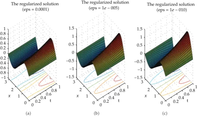
We have inFigure 2the graphs of the regularized solutionvδin·, t,i 4,5,6 and

n10.

We have in Figure 3 the graphs of the exact solution u·, t and of the regularized solutionvδin·, t,i7,8 andn10.

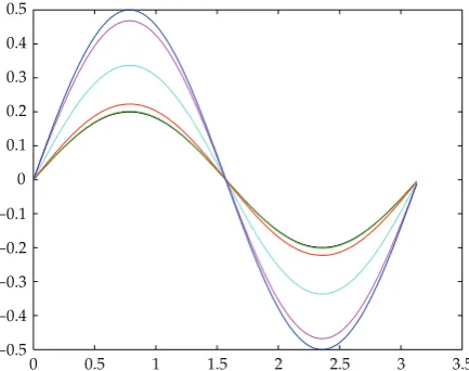
Now, Figure 4 can represent visually the exact solution and regularized solutions corresponding toδi,i1, . . . ,8 at initially timet0.

Notice that, inFigure 4, the curve number 0 expressing the exact solution is indistinguishable from the curve numberiexpressing the regularized solution corresponding toδi,i6,7,8.

Remark 3.1. From1.7and3.5, we obtain the exact solution corresponding to the measured

datagδx:

wx, t

∞

k1

0 0.2 0.40.6 0.81 0 1 2 3

−0.2

−0.15

−0.1

−0.05

0 0.05 0.1 0.15 0.2 t x

The regularized solution

(eps=0.1)

a 0 0.2 0.40.6 0.81 0 1 2 3

−0.2

−0.15

−0.1

−0.05

0 0.05 0.1 0.15 0.2 t x

The regularized solution

(eps=0.01)

b

−0.25

−0.2

−0.15

−0.1

−0.05

0 0.05 0.1 0.15 0.2 0.25 0 0.2 0.40.6 0.81 0 1 2 3 t x

The regularized solution

(eps=0.001)

c

Figure 1: The regularized solutions corresponding toδi,i1,2,3.

−1

−0.8

−0.6

−0.4

−0.2

0 0.2 0.4 0.6 0.8 1 t x 00.2 0.40.6 0.81 0 1 2 3

The regularized solution

(eps=0.0001)

a

0

−1.5

−1

−0.5

0.5 1 1.5

The regularized solution

(eps=1e−005)

t x 00.2 0.40.6 0.81 0 1 2 3 b 0

−1.5

−1

−0.5

0.5 1 1.5

The regularized solution

(eps=1e−010)

t x 0 0.2 0.40.6 0.81 0 1 2 3 c

Figure 2: The regularized solutions corresponding toδi,i4,5,6.

where

wkt ek

2_λT−λt

gδ,k−

_T

t

ek2λs−λtfkwsds,

fkws

2

π

_π

0

fx, s, wx, ssinkxdx,

gδ,k

2

π

_π

0

gδxsinkxdx.

0

−1.5 −1 −0.5 0.5 1 1.5

t x

00.2 0.40.6

0.81

0 1 2 3

The regularized solution

(eps=1e−020)

a

0

−1.5

−1

−0.5

0.5 1 1.5

t

x

00.2

0.40.6

0.81

0 1 2 3

The regularized solution

(eps=1e−050)

b

0

−1.5

−1

−0.5

0.5 1 1.5

t

x

00.2

0.40.6

0.81

0 1 2 3

The exact solution

c

Figure 3: The regularized solutions correspondingδi,i7,8 and the exact solution.

0 0.5 1 1.5 2 2.5 3 3.5

−0.5

−0.4

−0.3

−0.2

−0.1

0 0.1 0.2 0.3 0.4 0.5

Figure 4: The exact solution and the regularized solutions corresponding toδi,i1, . . . ,8 at initial time

t0.

Now, we cannot calculate the formula3.9exactlywe need to findfkwswhile

we have not knownw yet. FromTheorem 2.2, we use the iteration for3.9at initial time

t0 as follows:

wnω,0

∞

k1

Table 2

δ wδi5·,0−u·,0₂

δ110−1 1.1856e031

δ210−2 1.0e031

δ310−3 1.0e031

δ410−4 1.0e031

δ510−5 1.0e031

δ610−10 1.0e031

δ710−20 1.0e031

δ810−50 1.0e031

where

wknx,0 exp

2k2gδ,k−

₁

0

expk2s2sfkwn−1sds,

gδ,k

2

π

_π

0

gδxsinkxdx,

w1x,0 1δsinxcosx.

3.12

Then we get the error in theTable 2.

We can see that the errorwδi5·,0−u·,02is very large. Therefore, the problem is

ill-posed and a regularization is necessary.

Acknowledgment

All authors were supported by the National Foundation for Science and Technology DevelopmentNAFOSTED.

References

1 Z. Qian, C.-L. Fu, and R. Shi, “A modified method for a backward heat conduction problem,” Applied

Mathematics and Computation, vol. 185, no. 1, pp. 564–573, 2007.

2 R. E. Ewing, “The approximation of certain parabolic equations backward in time by Sobolev equations,” SIAM Journal on Mathematical Analysis, vol. 6, pp. 283–294, 1975.

3 X.-L. Feng, Z. Qian, and C.-L. Fu, “Numerical approximation of solution of nonhomogeneous back-ward heat conduction problem in bounded region,” Mathematics and Computers in Simulation, vol. 79, no. 2, pp. 177–188, 2008.

4 C.-L. Fu, X.-T. Xiong, and Z. Qian, “Fourier regularization for a backward heat equation,” Journal of

Mathematical Analysis and Applications, vol. 331, no. 1, pp. 472–480, 2007.

5 D. N. H`ao, “A mollification method for ill-posed problems,” Numerische Mathematik, vol. 68, no. 4, pp. 469–506, 1994.

6 A. Hasanov and J. L. Mueller, “A numerical method for backward parabolic problems with non-selfadjoint elliptic operators,” Applied Numerical Mathematics, vol. 37, no. 1-2, pp. 55–78, 2001. 7 D. D. Trong, P. H. Quan, and N. H. Tuan, “A quasi-boundary value method for regularizing nonlinear

ill-posed problems,” Electronic Journal of Differential Equations, vol. 2009, no. 109, pp. 1–16, 2009.

9 I. V. Mel’nikova and A. I. Filinkov, The Cauchy Problem. Three Approaches, vol. 120 of Monograph and

Surveys in Pure and Applied Mathematics, Chapman & Hall, London, UK, 2001.

10 D. D. Trong and N. H. Tuan, “A nonhomogeneous backward heat problem: regularization and error estimates,” Electronic Journal of Differential Equations, vol. 2008, no. 33, pp. 1–14, 2008.

11 D. D. Trong, P. H. Quan, T. V. Khanh, and N. H. Tuan, “A nonlinear case of the 1-D backward heat problem: regularization and error estimate,” Zeitschrift f ¨ur Analysis und ihre Anwendungen, vol. 26, no. 2, pp. 231–245, 2007.

12 P. H. Quan, D. D. Trong, L. M. Triet, and N. H. Tuan, “A modified quasi-boundary value method for regularizing of a backward problem with time-dependent coefficient,” Inverse Problems in Science and

Engineering, vol. 19, no. 3, pp. 409–423, 2011.

Submit your manuscripts at

http://www.hindawi.com

Hindawi Publishing Corporation

http://www.hindawi.com Volume 2014

Mathematics

Hindawi Publishing Corporation http://www.hindawi.com

Differential Equations

International Journal of

Volume 2014

Applied MathematicsJournal of

Hindawi Publishing Corporation

http://www.hindawi.com Volume 2014

Hindawi Publishing Corporation

http://www.hindawi.com Volume 2014

Mathematical PhysicsAdvances in

Complex Analysis

Hindawi Publishing Corporation

http://www.hindawi.com Volume 2014

Optimization

Hindawi Publishing Corporation

http://www.hindawi.com Volume 2014

Combinatorics

Hindawi Publishing Corporation

http://www.hindawi.com Volume 2014 International Journal of

Journal of

Hindawi Publishing Corporation

http://www.hindawi.com Volume 2014

Function Spaces

Abstract and Applied Analysis

Hindawi Publishing Corporation

http://www.hindawi.com Volume 2014

International Journal of Mathematics and Mathematical Sciences

Hindawi Publishing Corporation http://www.hindawi.com Volume 2014

The Scientific

World Journal

http://www.hindawi.com Volume 2014

Discrete Dynamics in Nature and Society

Hindawi Publishing Corporation

http://www.hindawi.com Volume 2014

Discrete Mathematics

Hindawi Publishing Corporation

http://www.hindawi.com Volume 2014

Hindawi Publishing Corporation

http://www.hindawi.com Volume 2014