R E S E A R C H
Open Access
Further results on robust stability for
uncertain neutral systems with distributed
delay
Tao Wu
1, Lianglin Xiong
1,2*, Jinde Cao
2and Xinzhi Liu
3*Correspondence:
[email protected] 1School of Mathematics and Computer Science, Yunnan Minzu University, Kunming, China 2School of Mathematics, Southeast University, Nanjing, China Full list of author information is available at the end of the article
Abstract
This paper studies the problem of robust stability for uncertain neutral systems with distributed delay. By utilizing the incorporation of a new integral inequality technique and a novel Lyapunov–Krasovskii functional, some reduced conservative
delay-dependent stability conditions for asymptotic stability are established. Then some special cases of neutral systems are discussed. Based on these delay-dependent stability conditions, the condition for robustness is obtained for uncertain linear delayed systems. All these stability conditions are given in terms of linear matrix inequalities (LMIs), which can easily be computed by the LMI toolbox of Matlab. Finally, several examples are discussed in detail to display the usefulness and superiority of the obtained results.
Keywords: Robust stability; Uncertain neutral delayed system; Delay-dependent stability; Lyapunov functional; Linear matrix inequalities
1 Introduction
The stability analysis of neutral delay-differential systems has received considerable at-tention over the decades [1–18]. In the literature [1–18], the W-transform approach [1], the positivity-based approach [2–16], the characteristic equation method [17], the Lya-punov technique [18], and the state trajectory approach have been utilized to derive suf-ficient conditions for asymptotic stability and exponential stability of the systems. How-ever, most of the criteria are expressed in terms of a matrix norm or matrix measure of the system matrices. Unfortunately, the matrix norm operations usually make the crite-ria more conservative. Also the critecrite-ria in recent studies [16–18] require strong assump-tions such as that the matrix measures of system matrices have to be negative. These as-sumptions often make it difficult to apply the criteria to various systems, such as neu-tral delay-differential systems with time-varying delay, uncertain neuneu-tral delay-differential systems with time-delay, and so on. Inversely, these problems can easily be solved via the Lyapunov–Krasovskii functional (LKF) method, and this method has thus received con-siderable attention in the area of control engineering (see [19–23]).
As is well known, the Lyapunov functional method has received more and more atten-tion in recent years due to its effectiveness in many problems, such as the problem of control for linear neutral systems, the problem of delay-dependent stability (DDS) for
ear neutral systems (LNSS), etc. Based on this method, many interesting results on less conservative DDS conditions have been obtained (see, e.g., [24–42]). It is worth noting that [24–30,42] mainly considered the neutral and discrete delay. In fact, a lot of practical applications are modeled by systems with distributed delay. Consequently, a large number of stability and stabilization results on systems with distributed delay have been reported in [31–40]. It is pointed out that, although the information of three kinds of time-delays were considered in [32–37], the relationships between the three kinds of time-delays have not been fully studied. Accordingly, their interrelationships are discussed in [41]. How-ever, so far, the obtained maximum allowable upper bounds (MAUBs) of delay in [41] are not the best results. Thus, there still exists some room to improve with some novel LKFs, which combines with a new inequality technique.
On the other hand, DDS conditions are often obtained by the Lyapunov functionals theorem accompanied by some important techniques. Many important methods include the bounding inequalities for the cross term [24], a descriptor model transformation [25], the free-weighting matrix technique [26], integral inequality (II) methods (see [27,28,42]), delay decomposition [29], and discretized LKFs [30]. Generally speaking, the II method has always played a very important role in acquiring a DDS condition.
Up to now, many outstanding efforts have been made focused on the investigation of integral inequalities to decrease the conservatism of stability criteria. As an option of the Jensen inequality [25], the Wirtinger-based inequality was presented [43], in which the single integral information of the state is considered. Recently, the free-matrix based II was proposed in [44] by introducing some free matrices, which may be considered as an improved version of the Wirtinger-based inequality. More recently, the double integral information and triple integral information of the states was considered and a proposal was made [45] which could lead to more relaxed stability criteria for the systems. Spe-cially, it is noted that in order to further reduce the conservatism, some triple integral functions have been added into the LKFs [45]. Very recently, [46] presented a series of single/multiple IIs which proved to be less conservative than the existing ones. With the results in [46], further less conservative results would be obtained based on some novel Lyapunov functionals. Hence, the IIs in [46] should not be ignored, because they maybe play a significant role in getting a delay-dependent stability condition for neutral systems with discrete and distributed delays.
Motivated by the above discussion, the uncertain LNSS with discrete and distributed delays will be considered in this article. By choosing some suitable IIs, a novel LKF is con-structed. Based on the Lyapunov stability theory, some DDS conditions are got in terms of LMIs. Moreover, some examples are given to display the superiority and low conservatism of our results.
2 Problem statement
Consider the uncertain LNSS with time-delay ⎧
⎨ ⎩ ˙
x(t) – B˙x(t–τ) = Ax(t) + A1x(t–h) + A2
t
t–rx(s)ds,
x(t) =φ(t), ∀t∈[–ρ, 0],ρ=max{τ,h,r},t≥0, (1)
wherex(t)∈Rnis the state vector,τ,handrrepresent the neutral, discrete and distributed delay, respectively. ρ=max{τ,h,r}, φ(t) is the initial condition function. B =B+B,
A=A+A, A1=A1+A1, A2=A2+A2.A,B,A1,A2are known constant matrices. A,A1,A2andBdenote the time-varying uncertainties, and the uncertainties are supposed to be norm-bounded and satisfy
A A1 A2 B
=DF(t)
Na Nb Nc Nd
, (2)
whereD,Na,Nb,NcandNdare known constant matrices, andF(t) is an unknown continu-ous time-varying matrix function and satisfiesFT(t)F(t)≤I. Furthermore, for system (1), in order to guarantee system (1) has asymptotic stability, we need to assumeB+B ≤1. The major object of this paper is to establish some less conservative stability and robust stability conditions (RSCSs) for system (1). Before giving the primary results of this article, some important lemmas are firstly introduced as follows.
Lemma 2.1([45]) For a given R> 0and any differentiable function w: [a,b]→Rn,the
following inequality holds:
b
a
wT(α)Rw(α)dα≥ 1 b–a
b
a
w(α)dα
T
R
b
a
w(α)dα
, (3)
b
a
wT(α)Rw(α)dα≥ 1 b–a
b
a
w(α)dα
T
R
b
a
w(α)dα
+ 3
b–aΩ¯
T
1RΩ¯1+ 5
b–aΩ¯
T
2RΩ¯2, (4)
where
¯
Ω1=
b
a
w(α)dα– 2
b–a
b
a b
β
w(α)dαdβ,
¯
Ω2=
b
a
w(α)dα– 6
b–a
b
a b
β
w(α)dαdβ+ 12 (b–a)2
b
a b
γ
b
β
w(α)dαdβdγ.
Lemma 2.2([46]) For a given R> 0and any differentiable function x: [a,b]→Rn,and
Mk∈R6n×n(k= 1, 2, 3, 4, 5),the following inequality holds:
– b
a ˙
xT(s)Rx˙(s)ds≤υTΩυ, (5)
where
υ=
xT(b) xT(a) 1
bav
T
1 b22
av
T
2 b63
av
T
3 24b4
av
T
4
Ω= 5
k=1 ba 2k– 1MkR
–1MT
k +sym{MkΠk}, ba=b–a,
v1=
b
a
x(s)ds, v2=
b
a b
θ
x(s)ds dθ, v3=
b
a b
θ
b
u
x(s)ds du dθ,
v4=
b
a b
θ
b
u b
v
x(s)ds dv du dθ, Π1=¯e1–e¯2, Π2=¯e1+e¯2– 2¯e3,
Π3=e¯1–e¯2+ 6e¯3– 6e¯4, Π4=e¯1+¯e2– 12e¯3+ 30e¯4– 20e¯5,
Π5=e¯1–e¯2+ 20¯e3– 90¯e4+ 140¯e5– 70¯e6,
¯
ei=
0n×(i–1)n In 0n×(6–i)n
, i= 1, 2, . . . , 6.
In the following, we will use Lemmas2.1and2.2to obtain some main results.
3 Main results
In this section, for the uncertain LNSS (1), we give some sufficient conditions to ensure its robust stability. Then, for the sake of convenient calculation, we rewrite system (1) as
⎧ ⎪ ⎪ ⎨ ⎪ ⎪ ⎩ ˙
x(t) =Ax(t) +A1x(t–h) +A2
t
t–rx(s)ds+Bx˙(t–τ) +Dp(t),
p(t) =F(t)q(t),
q(t) =Nax(t) +Nbx(t–h) +Nc t
t–rx(s)ds+Ndx˙(t–τ),
(6)
wherep(t)∈Rn,q(t)∈Rn. Now, the DDS conditions are presented by taking advantage of the new inequality technique and the novel constructed Lyapunov functionals.
Theorem 3.1 For given delaysτ, h and r,system (1)is robustly asymptotically stable,
if there exist positive definite matrices P∈R5n×5n,and H,Q
i,Ri∈Rn×n(i∈1, 2, 3),Q4∈
R2n×2nand any matrices N
k,Mk,Fk∈R5n×n(k∈1, 2, 3, 4)satisfying the following
inequal-ities:
Ψ =symΓ2TPΓ1
+eT1(Q1+Q2+rQ3)e1–eT2Q1e2–eT3Q2e3–reT12Q3e12
– 3rΩ1TQ3Ω1– 5rΩ2TQ3Ω2+Θ1TQ4Θ1–Θ2TQ4Θ2+heT0R1e0
+τeT
0R2e0+re0TR3e0+Ω3+Ω4+Ω5+ΣTHΣ–eT15He15< 0, (7)
where
Γ1=
eT1 eT3 heT6 τeT9 reT12
T ,
Γ2=
eT
0 eT5 eT1 –eT2 eT1 –eT3 eT1 –eT4
T ,
Ω1=e12– 2e13, Ω2=e12– 6e13+ 12e14, Θ1=
eT
1 eT0
T ,
Θ2=
eT3 eT5
T
, e0=Ae1+A1e2+rA2e12+Be5+De15,
υ1=
eT
1 eT2 eT6 eT7 eT8
T
, υ2=
eT
1 eT2 eT9 eT10 eT11
υ3=
eT
1 eT2 eT12 eT13 eT14
T
, Σ=Nae1+Nbe2+rNce12+Nde5,
Ω3=υ1T
4
k=1 h
2k– 1NkR –1 1 NkT
υ1+sym
υ1TNkEk
,
Ω4=υ2T
4
k=1 τ
2k– 1MkR –1 2 MTk
υ2+sym
υ2TMkDk
,
Ω5=υ3T
4
k=1 r
2k– 1FkR –1 3 FkT
υ3+sym
υ3TFkGk
,
E1=e1–e2, E2=e1+e2– 2e6, E3=e1–e2+ 6e6– 6e7,
E4=e1+e2– 12e6+ 30e7– 20e8,
D1=e1–e3, D2=e1+e3– 2e9, D3=e1–e3+ 6e9– 6e10,
D4=e1+e3– 12e9+ 30e10– 20e11,
G1=e1–e4, G2=e1+e4– 2e12, G3=e1–e4+ 6e12– 6e13,
G4=e1+e4– 12e12+ 30e13– 20e14,
ei=
0n×(i–1)n In 0n×(15–i)n
, i= 1, 2, 3, . . . , 15.
Proof Take the following LKF candidate:
V(t) =ηT1(t)Pη1(t) +
t
t–h
xT(s)Q1x(s)ds+
t
t–τ
xT(s)Q2x(s)ds
+ t
t–r t
θ
xT(s)Q3x(s)ds dθ+
t
t–τ
x(s) ˙
x(s) T
Q4
x(s) ˙
x(s)
ds
+ t
t–h t
θ
˙
xT(s)R1x˙(s)ds dθ+
t
t–τ
t
θ
˙
xT(s)R2x˙(s)ds dθ
+ t
t–r t
θ
˙
xT(s)R3x˙(s)ds dθ, (8)
where
η1(t) =
xT(t) xT(t–τ) t
t–hxT(s)ds t
t–τxT(s)ds
t
t–rxT(s)ds T
.
Define
ξ(t) =
xT(t) xT(t–h) xT(t–τ) xT(t–r) x˙T(t–τ) 1
hcT1 h22cT2
6
h3cT3 1τc
T
4 τ22cT5 τ63cT6 1rc T
7 r22cT8 r63cT9 pT(t)
T
, (9)
with
c1=
t
t–h
x(s)ds, c2=
t
t–h t
θ
x(s)ds dθ, c3=
t
t–h t
θ
t
u
x(s)ds du dθ,
c4=
t
t–τ
x(s)ds, c5=
t
t–τ
t
θ
x(s)ds dθ, c6=
t
t–τ
t
θ
t
u
c7=
t
t–r
x(s)ds, c8=
t
t–r t
θ
x(s)ds dθ, c9=
t
t–r t
θ
t
u
x(s)ds du dθ.
From (8), differentiatingV(t) leads to ˙
V(t) = 2η˙1T(t)Pη1(t) +xT(t)Q1x(t) +xT(t)Q2x(t) –xT(t–h)Q1x(t–h)
+hx˙T(t)R1x˙(t) –xT(t–τ)Q2x(t–τ) +rxT(t)Q3x(t)
– t
t–r
xT(s)Q3x(s)ds+
x(t) ˙
x(t) T
Q4
x(t) ˙
x(t)
–
x(t–τ) ˙
x(t–τ) T
Q4
x(t–τ) ˙
x(t–τ)
– t
t–h ˙
xT(s)R1x˙(s)ds
+τx˙T(t)R2x˙(t) –
t
t–τ
˙
xT(s)R2x˙(s)ds
+rx˙T(t)R3x˙(t) –
t
t–r ˙
xT(s)R3x˙(s)ds, (10)
where
˙
η1(t) =
˙
xT(t) x˙T(t–τ) xT(t) –xT(t–h) xT(t) –xT(t–τ) xT(t) –xT(t–r)T.
By notingη1(t) =Γ1ξ(t),η˙1(t) =Γ2ξ(t) andx˙(t) =e0ξ(t) and by utilizing (4), we obtain
– t
t–r
xT(s)Q3x(s)ds≤ξT(t)
–reT12Q3e12– 3rΩ1TQ3Ω1– 5rΩ2TQ3Ω2
ξ(t). (11)
Employing Lemma2.2to (10), it is not difficult to get
– t
t–h ˙
xT(s)R1x˙(s)ds≤ξT(t)Ω3ξ(t), (12)
– t
t–τ
˙
xT(s)R2x˙(s)ds≤ξT(t)Ω4ξ(t), (13)
and
– t
t–r ˙
xT(s)R3x˙(s)ds≤ξT(t)Ω5ξ(t). (14)
From the conditionFT(t)F(t)≤I, clearly, we have
pT(t)p(t)≤qT(t)q(t) =ξT(t)ΣTΣ ξ(t). (15)
Accordingly, there exists a matrixH> 0, such that the following inequality holds:
0≤ξT(t)ΣTHΣ ξ(t) –pT(t)Hp(t), (16)
From (10) to (16), one can obtain ˙
V(t)≤ξT(t)Ψ ξ(t).
By using the Schur complement, according to the condition (7), it is easy to see that the inequalityΨ < 0. Hence, by Theorem 1.3 in [19], system (1) is robustly asymptotically
stable. This completes our proof.
Remark 3.2 It is worthy to note that the construction on Lyapunov functionals in (8) is very creative. Firstly, the functional contains three single integrals and four dou-ble integrals based on the property of the neutral distributed delay systems. Secondly, functionals consider the cross influence between the state information x(t –τ), and its derivatives and the system. Thirdly, the constructed functionals introduce addi-tional state information because of the utilization of the inequalities in the above lemmas, such as h12
t t–h
t
θxT(s)ds dθ, 1 τ2
t t–τ
t
θxT(s)ds dθ, 1
h3 t
t–h t
θ
t
uxT(s)ds du dθ,
1 τ3
t t–τ
t
θ
t
uxT(s)ds du dθ,
1
r3 t
t–r t
θ
t
uxT(s)ds du dθ and so on. Since the information of the state can be fully utilized, the resulting stability criteria may be less conservative.
Remark3.3 In many practical systems, finding the MAUB onrorhfor differenthorrto analyze the stability of the distributed delay systems is also meaningful.
By utilizing a method like in Theorem3.1, one obtains the less conservative DDS crite-rion for the following system withh=r:
⎧ ⎨ ⎩ ˙
x(t) =Ax(t) +A1x(t–h) +A2
t
t–rx(s)ds,
x(t) =φ(t), ∀t∈[–σ, 0],σ=max{h,r},t≥0. (17)
Corollary 3.4 For given scalars h and r,system(17)is asymptotically stable,if there exist positive definite matrices P∈R3n×3n,Q
i∈Rn×n(i∈1, 2, 3),and R1,R2∈Rn×n,and any matrices Nk,Mk∈R3n×n(k∈1, 2)satisfying the following inequalities:
¯
Ψ =symΓ4TPΓ3
+eT1(Q1+Q2+rQ3)e1–eT2Q1e2–eT3Q2e3
–reT5Q3e5+heT0R1e0+reT0R2e0+Ω6+Ω7< 0, (18)
where
Γ3=
eT
1 heT4 reT5
T
, Γ4=
eT
0 eT1 –eT2 eT1 –eT3
T ,
e0=Ae1+A1e2+rA2e5, υ¯1=
eT
1 eT2 eT4
T
, υ¯2=
eT
1 eT3 eT5
T ,
Ω6=υ¯1T
2
k=1 h
2k– 1NkR –1 1 NkT
¯
υ1+sym
¯
υ1TNkEk
,
Ω7=υ¯2T
2
k=1 r
2k– 1MkR –1 2 MTk
¯
υ2+sym
¯
υ2TMkDk
,
D1=e1–e3, D2=e1+e3– 2e5,
ei=
0n×(i–1)n In 0n×(5–i)n
, i= 1, 2, 3, 4, 5.
Proof Choose LKF as follows:
˜
V(t) =ηT2(t)Pη2(t) +
t
t–h
xT(s)Q1x(s)ds+
t
t–r
xT(s)Q2x(s)ds
+ t
t–r t
θ
xT(s)Q3x(s)ds dθ+
t
t–h t
θ
˙
xT(s)R1x˙(s)ds dθ
+ t
t–r t
θ
˙
xT(s)R2x˙(s)ds dθ,
where
η2(t) =
xT(t) t
t–hxT(s)ds t
t–rxT(s)ds T
,
ξ1(t) =
xT(t) xT(t–h) xT(t–r) 1
h t
t–hxT(s)ds
1
r t
t–rxT(s)ds T
.
Combining (3) with (5), and following a similar line to Theorem3.1, it is not hard to obtain
the DDS criterion (18). The proof is completed.
In the case ofr=h, system (1) is rewritten as
˙
x(t) –Bx˙(t–τ) =Ax(t) +A1x(t–h) +A2
t
t–h
x(s)ds. (19)
Theorem 3.5 For given scalarsτ and h,system(19)is asymptotically stable,if there ex-ist matrices P∈R5n×5n,Q
1,Q2,R∈Rn×n,and any matrices Mk∈R6n×n(k∈1, 2, 3, 4, 5)
satisfying the following inequalities:
Φ=symΥ2TPΥ1
+eT1Q1e1–eT2Q1e2+eT0Q2e0–eT7Q2e7
+heT0Re0+υTΩυ< 0, (20)
where
Υ1=
eT1 heT3 h22eT4 h63eT5 h244eT6
T ,
Υ2=
eT
0 eT1 –eT2 h(eT1 –eT3) h 2 2(e
T
1 –eT4) h 3 6(e
T
1 –eT5)
T ,
e0=Ae1+A1e2+hA2e3+Be7,
ei=
0n×(i–1)n In 0n×(7–i)n
, i= 1, 2, . . . , 7.
Proof Consider the LKF candidate
¯
V(t) =ηT3(t)Pη3(t) +
t
t–h
xT(s)Q1x(s)ds+
t
t–τ
˙
xT(s)Q2x˙(s)ds
+ t
t–h t
θ
˙
xT(s)Rx˙(s)ds dθ, (21)
where
η3(t) =
xT(t) vT
1(t) vT2(t) vT3(t) vT4(t)
T
, v1(t) =
t
t–h
x(s)ds,
v2(t) =
t
t–h t
θ
x(s)ds dθ, v3(t) =
t
t–h t
θ
t
u
xT(s)ds du dθ,
v4(t) =
t
t–h t
θ
t
u t
v
xT(s)ds dv du dθ.
Define
ξ2(t) =
xT(t) xT(t–h) 1
hv T
1(t) h22v2T(t) h63vT3(t) 24h4vT4(t) x˙T(t–τ)
T .
By notingη3(t) =Υ1ξ2(t),η˙T3(t) =Υ2ξ2(t) andx˙(t) =e0ξ2(t), the derivative ofV¯(t) along the trajectory of system (19) is computed:
˙¯
V(t) = 2η˙3T(t)Pη3(t) +xT(t)Q1x(t) –xT(t–h)Q1x(t–h) +x˙T(t)Q2x˙(t)
–x˙T(t–τ)Q2x˙(t–τ) +hx˙T(t)Rx˙(t) –
t
t–h ˙
xT(s)Rx˙(s)ds. (22)
Using Lemma2.2, one can see that the following inequality holds:
– t
t–h ˙
xT(s)Rx˙(s)ds≤ξ2T(t) 5
k=1 h
2k– 1MkR –1MT
k +
5
k=1
sym{MkΠk}
ξ2(t). (23)
Therefore, by combining (22) and (23), one has ˙¯
V(t)≤ξ2T(t)Φξ2(t).
We proceed by applying the Schur complement, andΦis given in Theorem3.5. Thus, if Φ< 0 in (20) holds, it is easy to see thatV˙¯(t) < 0, which means that system (19) has
asymptotic stability. This completes the proof.
For system (19), if there exist uncertain matricesA,A1,A2andB, we may also obtain the sufficient condition to ensure the robustly asymptotically stability. Hence, we will consider the uncertain neutral delayed system as follows:
˙
x(t) – B˙x(t–τ) = Ax(t) + A1x(t–h) + A2
t
t–h
x(s)ds. (24)
From (24), by using similar techniques to Theorem3.1to handle the uncertainties, a robust asymptotic stability condition can be given as follows.
Corollary 3.7 For given scalarsτ and h,the uncertain system(24)with A1+A1= 0is robustly asymptotically stable,if there exist matrices P∈R5n×5n,Q1,Q2,R,K∈Rn×n,and any matrices Mk∈R6n×n(k∈1, 2, 3, 4, 5)satisfying the following inequalities:
¯
Φ=Φ+Σ¯TKΣ¯ –eT8K e8< 0, (25)
whereΦis defined in(20)and
e0=Ae1+hA2e3+Be7+De8, Σ¯ =Nae1+hNce3+Nde7,
ei=
0n×(i–1)n In 0n×(8–i)n
, i= 1, 2, . . . , 8,
where
ξ3(t) =
xT(t) xT(t–h) 1
hv T
1(t) h22vT2(t) h63vT3(t) 24h4vT4(t) x˙T(t–τ) pT(t)
.
Similar to the proof of Theorem3.1, Corollary3.7can be proved, so it is omitted here.
Remark3.8 This paper just discusses the delay-dependent stability criteria, in which some useful approach can be effectively used to analyze the stabilization for linear neutral sys-tems with time-delay. Moreover, the employed results and methods may be extended to many interesting dynamical models such as uncertain neutral systems with Markovian jumping parameters and uncertain neutral systems with nonlinear perturbations or time-varying delays.
Remark3.9 Although the asymptotic stability of system (1) is discussed in this paper, the exponential stability of system (1) can easily be obtained by using a similar proof in [53]. In fact, for a linear neutral system with time-delay, the asymptotic stability implies expo-nential stability.
4 Numerical examples
In this section, several examples are provided to illustrate the usefulness of the above re-sults.
Example4.1 Consider system (1) with the following parameters [32]:
A=
–0.9 0.2 0.1 –0.9
, A1=
–1.1 –0.2 –0.1 –1.1
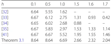
Table 1 The MAUB ofrforτ= 0.1 and different valueshin Example4.1
h 0.1 0.5 1.0 1.5 1.6 1.7
[image:11.595.128.397.206.362.2][32] 6.64 5.55 1.62 – – – [33] 6.67 6.12 2.75 1.31 0.93 0.42 [34] 6.65 6.02 2.68 0.88 – – [35] 6.67 5.83 2.97 1.53 1.33 1.14 [41] 6.67 6.67 5.52 1.95 1.55 1.46 Theorem3.1 8.64 8.64 6.69 2.66 2.32 2.04
Table 2 The MAUB ofhforτ= 0.1 and different valuesrin Example4.1
r 1 2 3 4 5 6
[32] 1.12 0.93 0.77 0.65 0.55 0.43 [33] 1.58 1.20 0.95 0.77 0.64 0.51 [34] 1.47 1.14 0.95 0.80 0.68 0.50 [35] 1.78 1.30 0.99 0.77 0.62 0.47 [41] 1.90 1.49 1.34 1.20 1.07 0.91 Theorem3.1 2.10 1.71 1.41 1.25 1.14 1.05
A2=
–0.12 –0.12 –0.12 0.12
, B=
–0.2 0
0.2 –0.1
,
D=I, Na=Nb=Nc=Nd= 0.1I.
For this example, supposeτ = 0.1, by applying Theorem3.1, one can obtain the MAUB onrandhfor differenthandr, which is enumerated in Table1and Table2, respectively.
Example4.2 Consider system (17) with the following parameters [41]:
A=
–0.9 0
0 –0.9
, A1=
–1 –0.12
0.12 –1
, A2=
–0.12 –0.12 –0.12 0.12
.
For this example, in the caseh= 1, the allowable delay bounds onrin [41] is computed as 11.05, but by Corollary3.4, we can get a larger delay bound, 11.21. Besides, in the caser= 1, the allowable delay bounds onhin [36,37] and [41] are computed as 1.8302, 2.8011 and 3.5823, respectively. However, by Corollary3.4, one can obtain a larger delay bound 3.9235, which are 114.375%, 40.070%, 9.524%more than that of [36,37] and [41], respectively. In addition, this example shows that our method in this paper is better than that in [36,37] and [41].
Example4.3 Consider system (19) with the following parameters whenB= 0:
A=
–2 0
0 –0.9
, A1=
–1 0
–1 –1
, A2= 0.
Table 3 Upper bound onhobtained for Example4.3
Methods hmax
(N= 1) [19] 6.059 (N= 2) [19] 6.165
[47] 6.1107
[43] 6.059
(N= 6) [48] 6.12
[49] 6.1664
[46] 6.1719
Theorem3.5 6.1725 The analytical bounds 6.1725
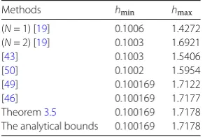
Table 4 Delay interval which stability of system in Example4.4is guaranteed
Methods hmin hmax
(N= 1) [19] 0.1006 1.4272 (N= 2) [19] 0.1003 1.6921 [43] 0.1003 1.5406 [50] 0.1002 1.5954 [49] 0.100169 1.7122 [46] 0.100169 1.7177 Theorem3.5 0.100169 1.7178 The analytical bounds 0.100169 1.7178
Example4.4 Consider system (19) with the following parameters whenB= 0:
A=
0 1
–2 0.1
, A1=
0 0
1 0
, A2=
0 0
0 0
.
SinceRe(eig(A+A1)) = 0.05 > 0, the system is unstable whenh= 0. Few linear matrix inequalities can test the stability condition of this system. This is so because the delay is distributed in some interval to guarantee the stability for the systems. Table4lists the results obtained from Theorem3.5and other conditions reported in the literature. From Table4, we can see that our maximum admissible upper bounds are the analytical bounds.
Example4.5 When the parameters of system (19) in this example is described as follows (B= 0):
A=
0.2 0
0.2 0.1
, A1= 0, A2=
–1 0
–1 –1
.
The corresponding delay bounds can also be given by computing the linear matrix in-equality in Theorem3.5. From Table5, in order to gain the MAUB to guarantee the system stability, various kinds of methods are proposed to calculate the MAUB. It is easily seen that our presented approach is best due to the fact that the obtained MAUB concerns the analytical bounds.
Example4.6 To show the comparison in more detail, the parameters of the system (19) in this example are given by [43] whenB= 0:
A=
0 1
–100 –1
, A1=
0 0.1
0.1 0.2
[image:12.595.225.372.238.336.2]Table 5 Upper bound onhobtained for Example4.5
Methods hmax
[37] 1.6339
[43] 1.8770
[50] 1.9504
[51] 2.0395
[49] 2.0395
[52] 2.0402
[46] 2.0412
Theorem3.5 2.0412 The analytical bounds 2.0412
Table 6 Upper bound onhobtained for Example4.6
Methods hmax
[50] 0.126 [51] 0.577 [52] 0.675 Theorem3.5 0.749
By using Theorem3.5, a larger delay bound 0.7495 is got. In order to show more clearly, Table6lists the computed upper bounds by unlike methods. It is easily observed that our method produces better result than the existing results.
Example4.7 Consider system (19) with the following parameters:
A=
–2 0
0 –0.9
, A1= 0, A2=
–1 0
–1 –1
, B=
–0.2 0
0.2 –0.1
.
[image:13.595.134.403.513.564.2]By Corollary 1 in [37], the system (19) is asymptotically stable for all delays h ∈
[0, 1.8536]. Applying Theorem3.5to this example, system (19) becomes asymptotically stable for all delaysh∈[0, 3.6574].
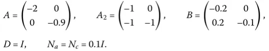
Example4.8 Consider system (24) with the following parameters:
A=
–2 0
0 –0.9
, A2=
–1 0
–1 –1
, B=
–0.2 0
0.2 –0.1
,
D=I, Na=Nc= 0.1I.
In the first place, we takeNd= 0. By Corollary 1 in [37], the system (24) is robustly asymptotically stable for all delaysh∈[0, 1.7174]. However, using Corollary3.7in this ex-ample, the interval of delayhsuch that the system (24) is robustly asymptotically stable is [0, 3.2314]. Then letNd= 0.1I, by Corollary 2 in [37], the system (24) is robustly asymp-totically stable forh∈[0, 1.4986]. However, by applying Corollary3.7, we can obtain the interval of delayh∈[0, 3.0175] which ensures the robust stability of system (24).
Example4.9 To show the comparison in more detail, the parameters of the system (19) in this example is given by [18]
A=
–3 –2
1 0
, A1=
0 α
α 0
, A2= 0, B=
0.1 0
0 0.1
whereαis a real parameter. In this example, we assumeτ =h= 1. By Theorems 2.5 and 2.6 in [18], it can be found that this system (19) is not only asymptotic but exponential for all|α| ≤0.6213. However, by Theorem3.5, it is computed that the maximum allowed value|α| ≤1. Therefore, Theorem3.5is less conservative than the results in [18].
5 Conclusion
Based on some new LKF and IIs, several new stability and RSCSs have been proposed for uncertain linear neutral system with time-delay. The obtained DDS conditions in this paper are of low conservatism owing to the constructed novel LKF, which combines with the new II technique. Besides, the problem of robust stability for uncertain systems with-out neutral or distributed term are commendably addressed. Moreover, some interesting examples have been presented to display the low conservatism of the derived DDS condi-tions by comparison with the existing results.
Acknowledgements
The authors would like to thank the reviewers for their comments and suggestions which help to improve the presentation of the paper.
Funding
This work was supported by National Natural Science Foundation under Grant 11461082, 11601474, 61573096, 61463050 and 61472093, supported by the Jiangsu Provincial Key Laboratory of Networked Collective Intelligence under Grant No. BM2017002, the key laboratory of numerical simulation of Sichuan Province, under Grant No. 2017KF002, Yunnan Provincial Department of Education Science Research Fund Project, under Grant No. 2018Y105, the Natural Science Foundation of Yunnan Province No. 2015FB113, Postgraduate Innovation Foundation of Yunnan Minzu University, under Grant No. 2018YJCXS225.
Competing interests
The authors declare that they have no competing interests.
Authors’ contributions
Each of the authors, TW, LLX, JDC and XZL, contributed to each part of this work equally and read and approved the final version of the manuscript.
Author details
1School of Mathematics and Computer Science, Yunnan Minzu University, Kunming, China.2School of Mathematics,
Southeast University, Nanjing, China.3Department of Applied Mathematics, University of Waterloo, Waterloo, Canada.
Publisher’s Note
Springer Nature remains neutral with regard to jurisdictional claims in published maps and institutional affiliations.
Received: 25 July 2018 Accepted: 12 November 2018
References
1. Azbelev, N.V., Simonov, P.M.: Stability of Differential Equations with Aftereffect. Stability and Control: Theory, Methods and Applications, vol. 20. Taylor & Francis, London (2003)
2. Briat, C.: Robust stability and stabilization of uncertain linear positive systems via integral linear constraints—Liand
L∞—gains characterizations. Int. J. Robust Nonlinear Control23(17), 1932–1954 (2013)
3. Buslowicz, M.: Robust stability of positive continuous time linear systems with delays. Int. J. Appl. Math. Comput. Sci. 20, 665–670 (2010)
4. Campbell, S.A.: Delay independent stability for additive neural networks. Differ. Equ. Dyn. Syst.9, 115–138 (2001) 5. Domoshnitsky, A., Sheina, M.V.: Nonnegativity of Cauchy matrix and stability of systems with delay. Differ. Uravn.25,
201–208 (1989)
6. Domoshnitsky, A., Fridman, E.: A positivity-based approach to delay-dependent stability of systems with large time-varying delays. Syst. Control Lett.97, 139–148 (2016)
7. Domoshnitsky, A., Shklyar, R.: Positivity for non-Metzler systems and its applications to stability of time-varying delay systems. Syst. Control Lett.118, 44–51 (2018)
8. Feyzmahdavian, H.R., Charalambous, T., Johansson, M.: Exponential stability of homogeneous positive systems of degree one with time-varying delays. IEEE Trans. Autom. Control59, 1594–1599 (2014)
9. Gyori, I., Hartung, F.: Fundamental solution and asymptotic stability of linear delay differential equations. Dyn. Contin. Discrete Impuls. Syst.13, 261–287 (2006)
11. Hofbauer, J., So, J.W.-H.: Diagonal dominance and harmless off-diagonal delays. Proc. Am. Math. Soc.128, 2675–2682 (2000)
12. Kaczorek, T.: Stability of positive continuous-time linear systems with delays. Bull. Pol. Acad. Sci., Tech. Sci.57, 395–398 (2009)
13. Liu, X., Yu, W., Wang, L.: Stability analysis for continuous-time positive systems with time-varying delays. IEEE Trans. Autom. Control55, 1024–1028 (2010)
14. Ngoc, P.H.A.: Stability of positive differential systems with delay. IEEE Trans. Autom. Control58, 203–209 (2013) 15. Bainov, D., Domoshnitsky, A.: Nonnegativity of the Cauchy matrix and exponential stability of a neutral type system
of functional-differential equations. Extr. Math.8, 75–82 (1993)
16. Domoshnitsky, A., Gitman, M., Shklyar, R.: Stability and estimate of solution to uncertain neutral delay systems. Bound. Value Probl.2014, 55 (2014)
17. Park, J.H., Won, S.: A note on stability of neutral delay-differential systems. J. Franklin Inst.336, 543–548 (1999) 18. Bˇastinec, J., Diblík, J., Khusainov, D.Y., et al.: Exponential stability and estimation of solutions of linear differential
systems of neutral type with constant coefficients. Bound. Value Probl.2010, Article ID 956121 (2010) 19. Gu, K., Kharitonov, V.L., Chen, J.: Stability of Time-Delay Systems, p. 12. Birkhäuser, Boston (2003)
20. Richard, J.P.: Time-delay systems: an overview of some recent advances and open problems. Automatica39(10), 1667–1994 (2003)
21. Kim, J.H.: Note on stability analysis of linear systems with time-varying delay. Automatica47(9), 2118–2121 (2011) 22. Park, P.G., Ko, J.W.: Stability and robust stability for systems with a time-varying delay. Automatica43(10), 1855–1858
(2007)
23. Sun, J., Liu, G.P., Chen, J., Rees, D.: Improved delay-range-dependent stability criteria for linear systems with time-varying delays. Automatica46(2), 466–470 (2010)
24. Park, P.: A delay-dependent stability criterion for systems with uncertain time-invariant delays. IEEE Trans. Autom. Control44(4), 876–877 (1999)
25. Fridman, E., Shaked, U.: An improved stabilization method for linear time-delay systems. IEEE Trans. Autom. Control 47(11), 1931–1937 (2002)
26. He, Y., Wu, M., She, J.H.: Delay-dependent robust stability and stabilization of uncertain neutral systems. Asian J. Control10(3), 376–383 (2008)
27. Sun, J., Liu, G.P., Chen, J.: Delay-dependent stability and stabilization of neutral time-delays systems. Int. J. Robust Nonlinear Control19(1), 1364–1375 (2009)
28. Gu, K.: An integral inequality in the stability problem of time-delay systems. In: Proceedings of the 39th IEEE Conference on Decision and Control, pp. 2805–2810 (2000)
29. Han, Q.L.: A discrete delay decomposition approach to stability of linear retarded and neutral systems. Automatica 45(2), 517–524 (2009)
30. Gu, K.: A further refinement of discretized Lyapunov functional method for the stability of time-delay systems. Int. J. Control74(10), 967–976 (2001)
31. Zheng, F., Frank, P.M.: Robust control of uncertain distributed delay systems with application to the stabilization of combustion in rocket motorchambers. Automatica38(3), 487–497 (2002)
32. Li, X.G., Hu, X.J.: Stability analysis of neutral systems with distributed delays. Automatica44, 2197–2201 (2008) 33. Sun, J., Chen, J., Liu, G., Rees, D.: On robust of uncertain neutral systems with discrete and distributed delays. In:
American Control Conference, Hyatt Regency Riverfront, St. Louis, MO, USA, June 10–12, pp. 5469–5473 (2009) 34. Hu, Y., Yu, K., Li, Y., Li, M.: Robust stability of uncertain systems with discrete and distributed delays. In: Proceedings of
the 29th Chinese Control Conference, pp. 1011–1015 (2010)
35. Chen, H.B., Zhang, Y., Zhao, Y.: Stability analysis for uncertain neutral systems with discrete and distributed delays. Appl. Math. Comput.218, 11351–11361 (2012)
36. Yue, D., Won, S., Kwon, O.: Delay dependent stability of neutral systems with time delay: an LMI approach. IEE Proc., Control Theory Appl.150(1), 23–27 (2003)
37. Chen, W.H., Zheng, W.X.: Delay-dependent robust stabilization for uncertain neutral systems with distributed delays. Automatica43(1), 95–104 (2007)
38. Qian, W., Liu, J., Sun, Y., et al.: A less conservative robust stability criteria for uncertain neutral systems with mixed delays. Math. Comput. Simul.80(5), 1007–1017 (2010)
39. Parlakci, M.: Robust stability of uncertain neutral systems: a novel augmented Lyapunov functional approach. IET Control Theory Appl.1(3), 802–809 (2007)
40. Chen, Y., Fei, S., Gu, Z., et al.: New mixed-delay-dependent robust stability conditions for uncertain linear neutral systems. IET Control Theory Appl.8(8), 606–613 (2014)
41. Chen, Y.G., Qian, W., Fei, S.M.: Improved robust stability conditions for uncertain neutral systems with discrete and distributed delays. J. Franklin Inst.352, 2634–2645 (2015)
42. Xiong, L., Zhang, H., Li, Y., Liu, Z.: Improved stabilization criteria for neutral time-delay systems. Math. Probl. Eng.2016, Article ID 8682543 (2016)
43. Seuret, A., Gouaisbaut, F.: Wirtinger-based integral inequality: application to time-delay systems. Automatica49(9), 2860–2866 (2013)
44. Zeng, H.B., He, Y., Wu, M., She, J.: Free-matrix-based integral inequality for stability analysis of systems with time-varying delay. IEEE Trans. Autom. Control60(10), 2768–2772 (2015)
45. Park, P.G., Lee, W., Lee, S.Y.: Auxiliary function-based integral inequalities for quadratic functions and their applications to time-delay systems. J. Franklin Inst.352, 1378–1396 (2015)
46. Chen, J., Xu, S., Zhang, B.: Single/multiple integral inequalities with applications to stability analysis of time-delay systems. IEEE Trans. Autom. Control62(7), 3488–3493 (2017)
47. Kao, C.Y., Rantzer, A.: Stability analysis of systems with uncertain time varying delays. Automatica43(6), 959–970 (2007)
48. Seuret, A., Gouaisbaut, F.: Complete quadratic Lyapunov functionals using Bessel–Legendre inequality. In: 2014 European Control Conference, ECC, Strasbourg, France, June 24–27, pp. 448–453 (2014)
50. Park, M.J., Kwon, O., Park, J.H., Lee, S.M., Cha, E.J.: Stability of time-delay systems via Wirtinger-based double integral inequality. Automatica55(5), 204–208 (2015)
51. Hien, L.V., Trinh, H.M.: Refined Jensen-based inequality approach to stability analysis of time-delay systems. IET Control Theory Appl.9(14), 218–219 (2015)
52. Zhao, N., Lin, C., Chen, B., Wang, Q.G.: A new double integral inequality and application to stability for time-delay systems. Appl. Math. Lett.65, 26–31 (2017)