R E S E A R C H
Open Access
Real-time CUDA-based stereo matching
using
Cyclops2
algorithm
Arnas Ivanavi
č
ius
1*, Henrikas Simonavi
č
ius
1, Julius Gel
š
vartas
1,2, Andrius Lauraitis
3, Rytis Maskeli
ū
nas
4,
Piotras Cimmperman
5and Paulius Serafinavi
č
ius
5Abstract
This paper presents a novel stereo matching algorithmCyclops2. The algorithm produces a disparity image, provided two rectified grayscale images. The matching is based on the concept of minimising a weight function calculated using the absolute difference of pixel intensities. We present three simple and easily parallelizable weight functions. Each presented function gives a different trade-off between algorithm processing time and reconstructed depth image accuracy. Detailed description of the algorithm implementation in CUDA is provided. The implementation was specifically optimised for embedded NVIDIA Jetson platform. NVIDIA Jetson TK1 and TX1 boards have been used to evaluate the algorithms. We evaluated seven algorithm variations with different parameter values. Each variation results in a different speed accuracy trade-off, demonstrating that our algorithm can be used in various situations. The presented algorithm achieves up to 70 FPS processing time on lower resolution images (750 × 500 pixels) and up to 23 FPS on high-resolution images (1500 × 1000 pixels). The use of optional post-processing stage (median filter) has also been investigated. We conclude that despite its limitations, our algorithm is relevant in the field of real-time obstacle avoidance.
Keywords:Stereo vision, Computer vision, Image processing, CUDA, GPU, Embedded systems
1 Introduction
The rapid advance of computational power has had a sig-nificant influence on the development of autonomous vehicles. Over the last decade, unmanned aerial vehicles (UAVs) and unmanned ground vehicles (UGVs) have been reaching higher degrees of autonomy, deploying more complex algorithms and sensors. Nonetheless, obstacle avoidance remains a challenge when considering real life applications. There are several types of sensors commonly used for 3D environment sensing and obstacle avoidance, such as light detection and ranging (LIDAR), structured-light, Time-of-Flight (TOF) and stereo cameras.
One of the most popular structured-light sensors often used in research is Microsoft’s Kinect. Structured-light sensors project known patterns onto the environment in order to estimate scene depth information. Structured-light sensors have successfully been used to solve many computer vision problems in indoor environments [1]. However, this approach has several limitations, namely
structured-light sensors do not work in direct sunlight and they have a limited detection range of 5 m.
TOF cameras, on the other hand, are less affected by direct sunlight because they use modulated light. Some TOF cameras have longer range than structured-light cameras but at the cost of increased power consumption. Another limitation of TOF cameras is low resolution of currently available sensors. The main advantage of TOF cameras is their very high frame rate (usually more than 100 Hz) [2].
LIDAR sensors, on the other hand, are often used in outdoor environments. These types of sensors have high accuracy and offer working ranges of up to 100 m. Main disadvantages of 3D LIDAR sensors are their low vertical resolution (for example 16 vertical channels) and very high price.
All of the discussed sensors are active, meaning they emit light rays in order to determine distances to objects in the environment. The biggest disadvantage of active sensors is their power consumption. Actively emitting light requires a lot of energy. Microsoft’s Kinect sensor consumes approximately 15 W of power. Stereo cameras are passive sensors; therefore, they consume less energy. * Correspondence:[email protected]
1Rubedo Sistemos, K. Baršausko st. 59a, Kaunas, Lithuania
Full list of author information is available at the end of the article
For example, stereo camera ZED from StereoLabs con-sumes only 2 W of power. Moreover, stereo cameras can adapt better to changing environment lighting condi-tions by controlling its gain and exposure parameters. Another advantage of passive sensors is that multiple sensors operating in the same environment do not inter-fere each other.
Stereo cameras usually consist of multiple sensors that work as one unit. Two or more video cameras can be used for this purpose. The main requirement is the calibration and synchronisation among all the devices within the sys-tem. It means that more than one image has to be proc-essed at a time in order to reconstruct a disparity map. A disparity map is an image where each pixel stores the shift of that pixel between two stereo images. A disparity map can be converted into a 3D point cloud using the camera parameters determined during the calibration. A 3D point cloud is a digital representation of the environment and can easily be used for path planning and obstacle avoid-ance. Stereo reconstruction is a computationally intensive procedure. Due to this fact, stereo matching is usually per-formed on powerful computers.
In recent years, with the graphics processing unit (GPU) technology becoming more affordable and powerful, NVI-DIA’s CUDA technology has been developed. It has opened up new opportunities for embedded systems which originally were not able to perform computationally intensive tasks in real time. Implementing a stereo match-ing algorithm in CUDA is a complex task. In some cases, it might even be impossible to implement a particular al-gorithm due to memory restrictions (especially on a low-end GPU). Moreover, most stereo matching algorithms have a trade-off between speed and accuracy.
Therefore, the aim of the carried research was to de-velop a stereo matching algorithm that would be oriented towards embedded systems and real-time applications. The presented algorithm concentrates on the speed aspect of stereo matching sacrificing accuracy where necessary.
Cyclops2 algorithm was evaluated on two embedded systems—NVIDIA’s Jetson boards—TK1 and TX1.
The paper is structured as follows. An overview of CUDA-based stereo matching algorithms is presented in Section 2. Section 3 describes the main principles of
Cyclops2 algorithm, its implementation and the experi-mental setup. The evaluation of results and discussion is presented in Section4and Section5respectively.
2 Related work
The main goal of this section is to compare stereo match-ing algorithms that support CUDA parallel computmatch-ing plat-form. The working principle of each algorithm is briefly described, highlighting their main advantages and disadvan-tages. Two metrics were used for algorithm comparison, namely the percentage of bad pixels (detailed description in
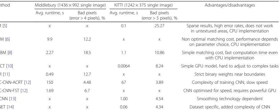
Section3.3) and algorithm runtime in seconds. The com-parison data was obtained from Middlebury version 3 [3] and KITTI Vision Benchmark [4] datasets. The comparison results are presented in Table1. Qualitative comparison of different algorithms is, however, complicated.
First, the threshold for bad pixels is different in Middle-bury and KITTI datasets. For MiddleMiddle-bury dataset pixels whose disparity error is more than 4 pixels are considered bad pixels (same threshold as that used to evaluate our algorithms). Whereas, in the KITTI dataset, bad pixels have disparity error of more than 3 pixels. Therefore, the percentage of bad pixels should be higher in KITTI data-set if two algorithms have identical performance.
Second, Middlebury and KITTI datasets are very differ-ent. The KITTI dataset contains outdoor images, whereas Middlebury contains only indoor images. Moreover, the resolutions of images in the datasets are different.
Third, comparison of the algorithm runtime is even more complicated. Both Middlebury and KITTI datasets mainly focus on accuracy of reconstructed disparity images. Researchers run algorithms on their own hardware and only submit computed disparity images and computation times. The hardware used for computation is different be-tween algorithms and runtime results are therefore difficult to compare.
Most stereo matching algorithms can be split into two stages, namely cost computation and stereo matching. The cost computation stage usually determines the simi-larity of image regions in stereo image pair, and stereo matching finds the pair of patches with the best match-ing score. In this paper, we mainly focus on cost compu-tation functions optimised for embedded GPU platforms NVIDIA Jetson TK1 and TX1.
Block matching (BM) is a classical and very simple ste-reo matching algorithm. Image blocks from two steste-reo images are compared using Summed Absolute Difference (SAD) error criterion and full scanline search for finding optimal block displacement. Full scanline search used in BM produces a lot of errors especially in untextured areas. This is usually addressed by running image pre-filters that remove untextured areas and adding matched pixel uniqueness criterion. Even with these measures, results produced by BM are sparse and have high bad pixel per-centage, i.e. 25.27%. BM can be easily parallelised due to its simplicity [5], but results of CUDA implementation are not submitted in Middlebury and KITTI datasets. Our algorithm is similar to BM in that we are also performing a full scanline search.
two matching cost penalties, namely P1 and P2. P1 is a penalty applied to the matching cost when disparity value of a current pixel changes by 1 pixel, and P2 is applied when disparity value of a current pixel changes by more than 1 pixel. This technique helps to reconstruct disparity values in untextured areas of stereo images. Choosing good parameter values can be challenging and has a big impact on algorithm performance. CUDA implementation of SGM is available in libSGM [7] library, but no evalu-ation data is available at the time of writing.
Despite its limitations, SGM has led to the develop-ment of many modern stereo matching algorithms. For example, Semi-Global Block Matching (SGBM) uses Semi-Global Matching from SGM algorithm but calcu-lates matching costs using SAD of image patches. At the moment, SGBM is one of the most widely used algo-rithms in real-time applications due to its fast processing times and quality of produced images. It is also imple-mented in many major computer vision libraries, such as OpenCV [8] and VisionWorks [9]. This was the main reason why we chose to use SGBM for result compari-son in this paper.
Embedded real-time stereo estimation via Semi-Global Matching on the GPU (CSCT) [10] is another method that uses Semi-Global Matching. The matching cost is computed using Center-Symmetric Census Transform and additionally median filter is used to remove outliers. This implementation was optimised for CUDA platform and achieves very good processing time of 0.0064 s on NVIDIA Titan X.
The Iterative Refinement Method for Adaptive Support-Weight Correspondences (IDR) method [11] has a strict binary assignment of weights near boundaries and uses a two-pass approximation of adaptive support weights for matching cost aggregation and an iterative refinement technique that enforces consistency of disparities. IDR
was the fastest method of those compared in Middlebury dataset, but the computations were performed on a powerful NVIDIA TITAN Black GPU. IDR’s average speed was 0.49 s and its percentage of bad pixels was 12.7%.
In recent years, convolutional neural networks (CNN) have become very popular in solving various computer vision problems, and stereo matching is not an excep-tion. In 2015, Stereo Matching by training a Convolu-tional Neural Network to Compare Image Patches (MC-CNN) [12] was one of the first methods utilising CNN and achieving bad pixel percentages lower than 7%. This algorithm has two network architectures (one optimised for speed (FST), other for accuracy (ACRT)). MC-CNN uses CNN for matching cost computation, and matching is performed using Semi-Global Matching from SGM. The success of MC-CNN has led to the adoption of CNN in modern stereo matching algorithms.
Efficient Deep Learning for Stereo Matching (C-CNN) [13] is a more advanced method that uses CNN not only for cost computation but also for predicting the disparity image values. A C-CNN-produced output is not competi-tive compared with other modern methods, and the authors are therefore using additional post-processing stages to improve the quality of produced disparity image.
A Large Dataset to Train Convolutional Networks for Disparity, Optical Flow, and Scene Flow Estimation DNET [14] is also a CNN-based approach that is trained to perform full disparity estimation task without requir-ing additional matchrequir-ing algorithms. This method recon-structs good disparity images that have only 4.34% of bad pixels. DNET also has a short processing time of 0.06 s. The main challenge of CNN-based stereo match-ing algorithms is that they require large datasets for training. This is usually addressed by synthetically gener-ating large datasets. The main disadvantage of most CNN-based methods is that even optimised versions of Table 1A comparison of CUDA-based stereo matching algorithms on Middlebury and KITTI datasets
Method Middlebury (1436 × 992 single image) KITTI (1242 × 375 single image) Advantages/disadvantages
Avg. runtime, s Bad pixels (error > 4 pixels), %
Avg. runtime, s Bad pixels (error > 3 pixels), %
BM [5] x x 0.1 25.27 Sparse results, high error rates, does not work
in untextured areas, CPU implementation
SGM [6] 9.9 12.2 x x Non optimal matching cost, performance depends
on parameter choice, CPU implementation
SGBM [8] 2.27 18.5 1.1 10.86 Simple matching cost, fast computation time even
with CPU implementation
CSCT [10] x x 0.0064 8.24 Simple GPU model, hard to adjust to complex tasks
IDR [11] 0.49 12.7 x x Strict binary weights near boundaries
MC-CNN-ACRT [12] 150 4.48 67 3.89 Complexity of training CNN, slow speed
MC-CNN-FST [12] 1.69 6.7 x x CNN optimised for speed, requires powerful GPU
C-CNN [13] x x 1.00 4.54 Smoothing technology dependent
these algorithms require powerful GPU processors (usu-ally NVIDIA Titan X). Therefore, these methods cannot be used on a low-power embedded GPU, such as NVI-DIA TX1.
3 Materials and methods
Cyclops2 is a stereo matching algorithm that produces a disparity image from two rectified grayscale images: left and right. Rectified stereo images satisfy epipolar con-straints; therefore, the corresponding pixel search only has to be performed along image rows. The algorithm at-tempts to find the disparity value that minimises a weight function. We define the weight function as follows:
w¼ fðs;y;xÞ;dmin≤s≤dmax ð1Þ
Here, y (image row) and x (image column) are pixel coordinates in the left camera image; the independent variable s denotes a shift in image columns of rectified left and right images, expressed in pixels.sbelongs to an interval which is chosen taking into account the charac-teristic of a physical setup. The interval is denoted by dmin and dmax, which correspond to minimum and
maximum disparities respectively. w is the matching weight between the (y, x) pixel in left camera image and (y, x−s) pixel in the right camera image. The produced disparity image satisfies the following equation:
dðy;xÞ ¼s: minðwðs;y;xÞÞ ð2Þ
Here, d (y, x) is each pixel in the computed disparity image. The value s that is assigned to each disparity image pixel (y, x) is chosen such that the weight function would have minimal value for that (y, x).A weight func-tion is used to determine the similarity of two pixels in the input images.
Progressively, three different weight functions have been investigated. Each of these weight functions will be presented as separate methods:
1. Minimum Difference (MD); 2. Region Minimum Average (RMA); 3. Minimum Neighbour Sum (MNS).
The weight function of each method is described in the following subsection.
3.1Cyclops2weight functions
The MD method can be described as a straightforward implementation of the absolute difference concept. It calculates an absolute difference between two specific pixels located in the left and right images. Here, the minuend is the intensity of the pixel located in the left image and the subtrahend is the intensity of the pixel
located in the shifted right image. The difference is then assigned as the value of functionf, at points,y,x:
f sð;y;xÞ ¼jL yð ;xÞ−R yð ;x−sÞ j; ð3Þ
Here, y and x correspond to a row and column of an image and L and R are matrices of the left and right images. The last step is to find a shift value for eachy,x
pair, i.e. for each pixel in the disparity image that mini-mises the function at that point. The shift value is then assigned as a disparity value.
On the other hand, the RMA method is based on the notion that a disparity value that is closer to the ground truth can be found by taking into account the absolute differences between the neighbouring pixels as well. The method works iteratively. Starting with N= 0, each iter-ation calculates the average of 2Nabsolute differences lo-cated in the same row until the end of the row is reached. The goal is to find the minimum average which would in-dicate the maximum correspondence of two regions. The weight function of RMA can be defined as follows:
f sð;y;x;NÞ ¼ 1
2N X2N
i¼0jL yð ;x−iÞ−R yð ;x−i−sÞj ð4Þ Here, N is varied from 0 to the value such that the following equation is satisfied:
x−2N−s>0 ð5Þ
This is done to ensure that the weight calculation func-tion never goes out of the image row.
The MNS method is different from the previous two methods in a few ways. First, the calculation of delta here can be represented as follows:
ΔI sð;y;xÞ ¼jL yð ;xÞ−R yð ;x−sÞ−LþRj: ð6Þ
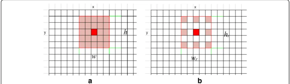
Hence, the delta function value at each shift and pixel is determined not only by the difference between pixel intensities, but also by the difference between the aver-age intensities. The weight function value is then ob-tained by summing up those deltas that fall into the bounds of a block. A block can be described as a kernel that has three parameters:
1. Kernel heighthorhr(odd);
2. Kernel widthworwr(odd);
3. Kernel stepks(greater than 0).
Therefore, a block is a data structure that has a rect-angular shape, i.e. it is an array of deltas with dimensions
1. Ifksequals 1, then the centre of the block is shifted
to the pointy,xand all the values that fit into a frame with dimensionsh×ware assigned (see Fig.1a);
2. Ifksis greater than one, then the array is filled, ignoring eachks−1 row and column, starting at
the centre pointy,x(see Fig.1b).
In the second case, the real size of a kernel can be cal-culated as follows:
wr¼ðks−1Þðw−1Þ þw;hr¼ðks−1Þðh−1Þ þh: ð7Þ
Lastly, the shift value that minimises the weight func-tion is calculated for eachy,xpair.
3.2 Implementation ofCyclops2
To obtain a stereo matching frame rate that would be suit-able for real-time applications, Cyclops2 algorithm has been oriented to utilise the GPU computational resources. Nevertheless, some portion of computations had to be delegated to the central processing unit (CPU).
Before going into further details, there are a few rules about the GPU programming that have to be addressed:
1. The main operations of an algorithm have to be performed concurrently; they have to be independent from one another or the dependence has to be minimised [15];
2. When NVIDIA CUDA technology is used, every memory access by threads has to be organised in such a way that read and write operations would be in the scope of neighbouring memory cells. Otherwise, cache memory gets updated, which leads to a significant increase of the processing time [15]; 3. NVIDIA’s CUDA architecture indicates that kernels
are executed concurrently by thread blocks. Each
block is divided into warps that consist of 32 threads. Threads inside a warp perform the same branch of the algorithm at the same time. Threads that belong to a warp but do not execute the same branch of the algorithm are executed sequentially. That being said, loops and conditional statements should be avoided when possible; 4. Shared memory is a unique memory on the
GPU shared among threads within a thread block. The size of a thread block on the newest GPUs is limited to 1024 threads [15].
Considering the rules above, we have created two implementations of the MNS method.
The first implementation consists of the main cycle per-formed on the CPU. The cycle is responsible for managing kernels and uploading data to the GPU memory. Each iteration of the cycle has its own shift value which leads to different deltas. Shifting the right image row with respect to the left image row is depicted in Fig.2.
In the cycle, two separate CUDA kernels were used: one for calculating absolute differences and the other for calculating weights and minimising its function. The main reason behind the separation is based on the fact that the performance of a thread block is maximised when threads interfere with fewer conditions and loops. The second operation is slightly more expensive com-pared with the first one. Therefore, in case of combin-ation, it would bring some of the threads to a halt.
Both kernels are called by the CPU specifying the number of threads per block and the size of a grid. The size of a block is determined by the size of an image. It was set to be a one-dimensional structure with a length equal to the quarter of an image width. In this case, the size of the grid is 4 × height.
Inside a grid, each thread has its own relative position. According to this position, individual pixels are accessed
and the absolute differences are calculated. When all the blocks within the grid have finished execution, another kernel is launched by the CPU, passing a pointer to the data stored on the GPU memory. The kernel responsible for the computation of weights has a loop that iterates through the specified neighbours of a pixel (see subsec-tion 3.1). It gathers the neighbouring deltas and aggre-gates their values. Then, the sum is compared with the latest weight value at pointy,x. If the current sum is lower than the previous, a new disparity value is assigned to that point. The same sequence of operations is repeated for every shift, overriding already set weights and disparities.
This approach does not use the advantages of the shared memory concept because it is performed on the global GPU memory. Accessing the global GPU memory is a more expensive operation, but it makes it possible to have kernels of various sizes, which leads to a more ver-satile algorithm implementation.
The second approach uses the CPU for uploading/ downloading data to/from the GPU, and there is only one CUDA kernel that is called by the CPU. The kernel for this purpose is loaded to the GPU, providing the size of a thread block that equals width of an image and the size of a grid that equals height of the image. An array of shared memory is then allocated dynamically, based on the size of the thread block. Inside the CUDA kernel, before doing any computation, images are loaded from the global GPU memory to the shared memory. It is done by reading individual pixels from the global ory and assigning them to the array of the shared mem-ory. The procedure is followed by the synchronisation of the threads within a block since the following steps re-quire the intensities (of a single image row) to be known. Then, each thread performs a loop, shifting a row of the
right image with respect to the left one. For each shift and point (y, x), the value of weight function is calcu-lated. The main difference compared with the previous approach is the fact that the height of a kernel is limited to 1 pixel and the width of the image is limited to 1024 pixels. It leads to a less favourable image quality, but the number of times the global GPU memory needs to be accessed is reduced.
3.3 Experimental setup
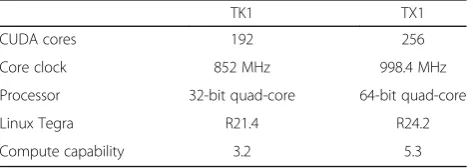
For a better overview, all experiments were performed on two separate embedded systems—NVIDIA Jetson de-velopment boards—TK1 and TX1. A side-by-side com-parison of their main specifications is shown in Table2.
The evaluated algorithms used both the CPU and GPU computations. The performance of each system was maximised by disabling the CPU power saving func-tionality and setting the GPU clock to the maximum frequency. The boards were powered using the default power adaptors provided with the development kits. Dur-ing the experiments, only the algorithm evaluation process was running.
Cyclops2 was compared with only one algorithm, SGBM, because it was one of the fastest algorithms in the Middlebury evaluation table that had a publicly Fig. 2Illustration of the basic concept of Cyclops2 algorithm. Right and left image rows are first shifted by specified number of columns. Shifted rows are subtracted to produce deltas. Deltas that correspond to minimal weight are used to fill disparity image with current shift value
Table 2Specifications of Jetson boards
TK1 TX1
CUDA cores 192 256
Core clock 852 MHz 998.4 MHz
Processor 32-bit quad-core 64-bit quad-core
Linux Tegra R21.4 R24.2
available GPU implementation. VisionWorks provided the most popular and stable implementation [9]; there-fore, it was used for the performance tests.
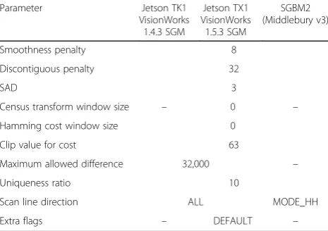
The VisionWorks implementation had a slightly different interpretation of its parameters for a better GPU adapta-tion. Also, both Jetson boards had different VisionWorks versions available. Nonetheless, the SGBM algorithm was configured to have similar parameters (see Table 3), which led to similar error-wise performance.
Cyclops2 (particularly the MNS method) has several parameters to play with (see subsection3.1). Five differ-ent versions of MNS were selected (see Table4) to
dem-onstrate the impact various parameters have on
performance. There is one parameter that has not been introduced yet, namely a step of disparity shift. Ordinar-ily, stereo matching algorithms consider each integral number that belongs to a disparity range. In this case, a step of disparity shift equals 1 pixel, which means that there are as many shifts as integral values in the interval. If the step is an integral number greater than 1 pixel, then every time one input image is shifted with respect to the other, by this number, the algorithm ignores in-between disparity values.
Both SGBM and Cyclops2 were evaluated using the method provided by Middlebury dataset version 3 [3] providing evaluation tools and images. It has a specific procedure, scripts, file formats, criteria and images. The most recent Middlebury version has three identical data-sets that differ in resolution:
1. Quarter (Q) resolution dataset. Quarter resolution images have up to 750 × 500 pixels and no more than 200 disparity values;
2. Half (H) resolution dataset. Half resolution images have up to 1500 × 1000 pixels and no more than 400 disparity values;
3. Full (F) resolution dataset. Full resolution images have up to 3000 × 2000 pixels and no more than 800 disparity values.
Each dataset has two parts: a training set and a test set with 15 image pairs each. The training set can be used to evaluate the error rate because each image pair comes with a ground truth disparity. Also, Middlebury provides the maximum disparity values of each image individu-ally. However, only the algorithms that have been pub-lished can be evaluated with the test set.
We used only quarter and half resolution training sets because full resolution images were too large for the Jetson embedded systems to process. There are many metrics available in the Middlebury stereo evaluation website. However, we decided to use only the following, as they provided enough information to compare the algorithms:
1. Algorithm computation time. As the Middlebury evaluation procedure states, it was measured without considering the time taken to load input images and save the result. The computation time was calculated for each image individually. Section
4provides the average algorithm computation time per image together with frames per second; 2. Percentage of bad pixels whose disparity
error is greater than 4.0 pixels. The provided measure is the average percentage of bad pixels per image. As already mentioned in introduction, the methods presented in this paper concentrate on optimising algorithm processing time at a cost of higher percentage of errors. This is reflected in the choice of higher than default bad pixel threshold (4.0 pixels instead of 2.0 pixels default of Middlebury dataset) which is more suitable in obstacle avoidance scenario;
3. Percentage of invalid pixels per image. These are pixels where the stereo matching algorithm was not
Table 3SGM parameters for different VisionWorks versions, side by side with the SGBM parameters that are presented in the Middlebury evaluation table
Parameter Jetson TK1
VisionWorks 1.4.3 SGM Jetson TX1 VisionWorks 1.5.3 SGM SGBM2 (Middlebury v3)
Smoothness penalty 8
Discontiguous penalty 32
SAD 3
Census transform window size – 0 –
Hamming cost window size 0
Clip value for cost 63
Maximum allowed difference 32,000 –
Uniqueness ratio 10
Scan line direction ALL MODE_HH
Extra flags – DEFAULT –
Table 4Cyclops2MNS methods and their relevant parameters used in the evaluation
Algorithm Parameters Step of disparity shift Kernel heighth Kernel widthw Kernel step ks
Note
MNS1 1 5 5 2 Only for quarter
resolution
MNS2 4 1 7 3
MNS3 4 1 7 3 Uses shared
memory. Only for quarter
resolution
MNS4 2 5 5 4 Only for half
resolution
able to estimate a disparity value. The provided measure is the average percentage of invalid pixels per image;
4. Average error of bad pixels per image. The average disparity value error of pixels that have been classified as bad pixels.
4 Results
One of the most important criteria used to evaluate the capability of an algorithm is the computation time. It can be represented as either seconds per frame or frames per second. In order to support the Middlebury evaluation method, the processing speed will be expressed in seconds. However, majority of our algo-rithm modifications had processing times in the order of milliseconds. Also, when working with real-time oriented computer vision applications, it is customary to present the computation time as frames per second (FPS). For these reasons, the processing speed will also be expressed in FPS.
We first compare the methods of Cyclops2
men-tioned in section3.1. The MD method yields high pro-cessing frame rate (see Table 5) at the expense of disparity image quality (see Fig. 3). Conceptually, it is due to the fact that the weight function of this method is simple. It considers only the intensity difference of 1 pixel, which, as we can see, is only enough to detect unique parts of the objects in the scene. Other pixels
are mismatched since there are a lot of pairs in the images that have similar differences.
RMA has approximately the same frame rate as MD (see Table 5). The core difference between the two is that RMA searches for a value that minimises the whole region rather than a single pixel. RMA recon-structs the shape of larger objects in the scene better than MD (see Fig. 4). This is mainly due to the fact that larger regions are usually more unique than small regions. However, the edges of objects in the disparity map become scattered.
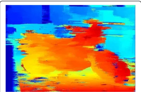
Compared with the previous methods, the quality of the MNS method is arguably better for robot naviga-tion (see Fig. 5). The basic shape of objects can be detected and there is less noise compared with that of RMA. However, small objects and shapes are filtered Table 5The average frame rate and processing time of each
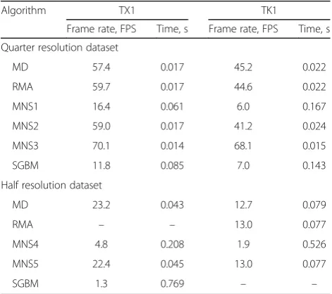
algorithm. Evaluation was performed on both Jetson boards. The RMA method was not performed on Jetson TX1 board with H resolution. The SGBM algorithm was not performed on TX1 with H resolution
Algorithm TX1 TK1
Frame rate, FPS Time, s Frame rate, FPS Time, s
Quarter resolution dataset
MD 57.4 0.017 45.2 0.022
RMA 59.7 0.017 44.6 0.022
MNS1 16.4 0.061 6.0 0.167
MNS2 59.0 0.017 41.2 0.024
MNS3 70.1 0.014 68.1 0.015
SGBM 11.8 0.085 7.0 0.143
Half resolution dataset
MD 23.2 0.043 12.7 0.079
RMA – – 13.0 0.077
MNS4 4.8 0.208 1.9 0.526
MNS5 22.4 0.045 13.0 0.077
SGBM 1.3 0.769 – –
Fig. 3Disparity image produced using the MD method. Overall object shape is visible in MD method output, but the image contains many noisy pixels. Incorrect pixels are visible on both foreground and background pixels
out, which could be a disadvantage in some scenarios. The results depend not only on the weight function, but also on its parameters. It is worth pointing out that MNS performs better on larger objects, since the weight function considers neighbouring differences. MNS has a slightly increased processing time caused by greater number of differences that have to be calcu-lated (see Table5).
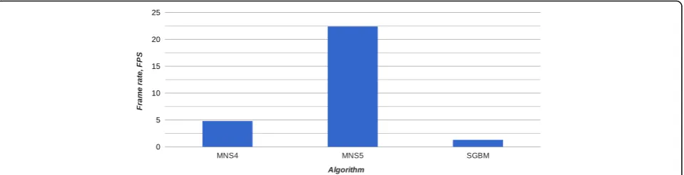
The processing speed comparison of several Cyc-lops2 modifications and SGBM algorithm can be seen in Figs. 6 and7.
Based on the two charts above, one can conclude that the computation time of MNS increases significantly with the size of a kernel (more processing). Whereas, increas-ing the step of disparity shift can reduce the amount of performed computations.
On quarter resolution images and TX1 board, MNS1, being the slowest modification, has 3.5 times lower frame rate compared with the fastest—MNS3. Nevertheless, MNS1 was 1.4 faster than SGBM. MNS3 has the same parameters as MNS2, but MNS3 was
implemented using the shared memory approach (see
subsection 3.2). Shared memory implementation
produces disparity images 1.2 times faster on average, compared with its non-shared memory implementa-tion. The fastest modification of MNS, namely, MNS3, is about 18 times faster than SGBM.
The results of the H training set suggest that SGBM computational times increase exponentially with reso-lution. Cyclops2, on the other hand, still manages to operate with a high frame rate. Detailed results of the processing speed are presented in Table5.
A comparison between TX1 and TK1 processing speed is shown in Fig.8.
The chart of Fig.8 signifies the core principle of the GPU performance optimisation. As expected, the majority of the algorithms perform significantly faster on the newer board due to its more advanced hard-ware. Depending on the Jetson board, the frame rate of the same algorithm can differ up to 2.5 times. Meanwhile, the shared memory modification of the algorithm seems to yield similar processing times. The reason for this similarity lies in the interaction between the CPU and GPU. The shared memory modification minimises CUDA kernel calls by the CPU and reads from the global GPU memory less often. It ensures a high processing rate even for a less powerful board.
It is worth mentioning that the VisionWorks imple-mentation of SGBM was not able to process half reso-lution training set images on Jetson TK1. The process terminated whenever the size of the image was close to 1500 × 1000 pixels. This is caused by the GPU driver timeout pre-set that works as a safety switch for many systems. Whenever the GPU does not report back to the OS within a specified time, the OS re-starts the GPU driver automatically. This is a stand-ard behaviour of NVIDIA GPU driver under Linux operating system.
The implementation of SGBM is targeting systems that have more computational power. Therefore, it is Fig. 5Disparity image produced using the MNS1 method. MNS1 is
able to reconstruct the shapes and spatial locations of the objects in the scene. This method produces significantly less noise than other presented methods
not possible to use SGBM for real-time applications with half resolution images on embedded systems. Same ap-plies to RMA and Jetson TX1 board, as RMA compares pixels iteratively until it reaches the number of pixels in a row. For large images, it requires a lot of time to per-form this procedure, so it gets terminated by the OS.
Next, the average percentage of bad and invalid pixels in the produced disparity images were evaluated. The re-sults of the experiment are presented in Figs.9and10.
The percentage of bad pixels in the disparity image
produced by the MNS method is kernel-size
dependent. Approximately, it belongs to the interval 46–77%. Similar error-wise quality can be obtained for both resolutions. There are a few reasons why the results of the same MNS modifications performed on both resolutions are not presented. First, it was noted that for higher resolution images, the step of a kernel has to be increased in order to obtain better quality. Second, for higher resolutions, the higher shifting step gives better results in terms of the processing time, where the quality of produced disparity images does not change at the same rate. Eventually, there is a trade-off between accuracy and frame rate that has to be made when considering a specific application.
Compared with SGBM, MNS produces up to 3–6 times more disparity values that have error greater
than 4 pixels. Nevertheless, unlike SGBM, MNS esti-mates disparity values of every pixel; therefore, its per-centage of invalid pixels is 0. More detailed results are shown in Table6.
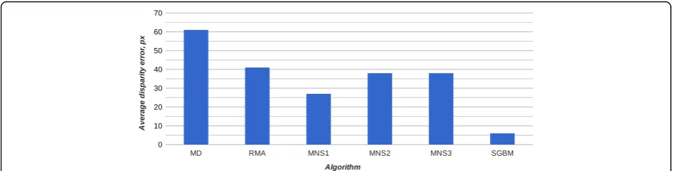
Another important metric for evaluating stereo match-ing algorithm quality is the average disparity error of bad pixels. The results of this evaluation are presented in Figs.11and12.
SGBM has a lower rate of average error compared with that of our proposed algorithm. The error of SGBM increases with resolution. Cyclops2 MNS algo-rithm has its bounds for the average error. The upper limit is the error of the MD method, and the lower limit is the error of MNS with the largest kernel size, which indicates that MD is a simplified MNS that has a kernel size of 1 pixel. Within these bounds, the parame-ters can be manipulated in order to achieve the desired processing time. That being said, the average error of MNS is considerably higher than that of SGBM. The main reason for such high percentage of bad pixels and average error is the fact that the weights are calculated using only the intensities of a grayscale image and their differences. This information is insufficient to match two points more accurately. The proposed methods are oriented towards higher frame rates, and higher errors are therefore tolerable.
Fig. 7The average frame rate of all training images. Evaluated on the H resolution training set using Jetson TX1
In order to increase the quality of the produced dis-parity images, a median blur filter was used as a post-processing stage. OpenCV 3.1.0 [8] implementa-tion of median blur was applied to the produced disparity images.
For quarter resolution images, median blur with ker-nel size of 3 pixels was used, for half resolution im-ages—5 pixels. The improvement on the average error for both resolutions can be seen in Figs.13and14.
Post-processing quarter resolution images had a sig-nificant impact on the output of those methods that produce relatively noisy disparities, e.g. MD's average error was reduced by 23%. Whereas for MNS1, being
the most accurate Cyclops2 method (Q resolution)
(see Table 5), only 7% error reduction was observed. On the other hand, MNS4, the most accurate modifi-cation (H resolution) of Cyclops2, gets the average error reduction of 34%, while MNS5 gets only 11%. The reason of such difference is that MNS5 had a smaller kernel and a larger shift step compared with that of MNS4. The results of MNS5 were too scat-tered for the post-processing to make a greater im-provement, as the median blur filter simply removes outliers.
More detailed results together with the added latency are presented in Table7.
Based on the results of both Table 7and Table 5, we can conclude that Jetson TK1 processing speed decreases up to two times after applying the suggested post-processing. On the other hand, the procedure has a less significant impact on the Jetson TX1 board pro-cessing time. It is mainly because the blur is per-formed on the CPU and TX1 has a better one. The added latency on TX1 for both resolutions differs up to 10 times, while on TK1—up to 21.
5 Discussion
The algorithm presented in this paper was optimised for high processing frequency, making it usable in real-time applications, such as obstacle detection and avoidance. The implementation was targeted for NVI-DIA Jetson embedded platforms. These platforms are optimised for low power consumption and are there-fore well suited in robotics applications.
The computational simplicity of the proposed algo-rithm made it possible to parallelise it efficiently using CUDA technology. The main disadvantage of the pro-posed algorithm is high percentage of bad pixels. On Fig. 9Average percentage of bad pixels, whose error is larger than 4 pixels, and average percentage of invalid pixels. Evaluation performed using Q resolution training set images
average, more than half of the points in the produced disparity image have an error greater than 4 pixels. The error tolerance of a stereo matching algorithm de-pends on a specific use-case and operating environ-ment. For example, in a controlled environment, where a robot is only likely to encounter big obstacles, a higher than currently selected (4 pixels) threshold would be tolerable. The accuracy versus speed trade-off of our algorithm is adjustable by tuning its parame-ters and can be tuned for different use-cases.
An alternative solution for reducing bad pixel per-centage is to use pre-processing filters and additional matching pixel uniqueness checks, such as those used in the BM algorithm. The pre-processing filter removes untextured regions from the original left and right images so that these regions would not produce erroneous disparities. The uniqueness check stage ensures that the matching pixel weight is sig-nificantly different from the weight of the second best
matching pixel. Both of these techniques would re-quire additional computations that would have a sig-nificant impact on the performance of the algorithm. Furthermore, pre-processing filters and uniqueness checks do not solve the problem of incorrect matches but instead reduce the percentage of bad pixels by in-creasing the percentage of invalid pixels.
The majority of errors produced by our algorithm are due to the fact that the disparity values are calcu-lated only using neighbouring pixel intensities. This could be improved by taking into account already cal-culated disparities of the neighbouring pixels. Neigh-bouring disparities can be used to take into account the fact that real objects are usually regions and not individual points. This can be done by incorporating additional terms into the current weight function. These terms, for example, could be the distance to the nearest edge, region, etc. The neighbouring pixel disparities can also be incorporated by using more sophisticated matching techniques, such as that used in SGM. This, however, is a non-trivial task and would most certainly have significant performance cost mainly due to additional memory being accessed by the algorithm.
Another approach is to use post-processing algo-rithms to remove outliers. This is usually implemented by filtering the produced disparity image with a median blur or Gaussian blur filters. For some modifi-cations of our proposed algorithm, the suggested median filter post-processing reduced the average error by 34%. Median filter is a commonly used post-processing algorithm that has not been observed to significantly decrease object locality accuracy. More-over, this method is successfully being used by the top-ranking algorithms, such as MC-CNN. The main disadvantage of additional post-processing stages is the added computational time.
The proposed algorithm was evaluated using Mid-dlebury dataset. The algorithm showed competitive processing time results despite the fact that it was Table 6The average quality measures of each algorithm
performed on the Q and H resolution training sets images
Algorithm Bad 4.0, % Invalid, % Average error, pixel
Quarter resolution dataset
MD 89.0 0.0 61
RMA 77.4 0.2 41
MNS1 46.4 0.0 27
MNS2 72.9 0.0 38
MNS3 72.9 0.0 38
SGBM 12.1 6.6 6
Half resolution dataset
MD 89.4 0.0 61
RMA 78.3 0.1 42
MNS4 47.5 0.0 38
MNS5 76.5 0.0 43
SGBM 8.7 9.7 7
evaluated on an embedded NVIDIA Jetson platform. Evaluating the algorithm using the KITTI dataset would have provided additional insights of its per-formance on the outdoor environment images.
6 Conclusions
The aim of this paper is to present a novel stereo match-ing algorithmCyclops2. The algorithm performs scanline correspondence search and minimises a simple weight function. The weight function values are calculated using absolute difference of pixel intensity values. We described three different weight functions, namely MD, RMA and MNS. MD is a very simple method only taking single pixel intensities into account. RMA and MNS are more sophisticated methods that incorp-orate the neighbouring pixel information. Presented functions can be used to adjust stereo matching per-formance for a specific use-case.
The proposed algorithm was implemented using CUDA parallel programming library and optimised for embedded NVIDIA Jetson platform. This paper discusses the rules that should be followed when optimising algorithms for parallel GPU execution. We provide detailed algorithm implementation de-scription. Two algorithm versions have been imple-mented. The first version used CPU loops and two
GPU kernels, whereas the second used a single GPU kernel and GPU shared memory.
Cyclops2 has been evaluated on two NVIDIA Jetson boards, namely TK1 and TX1. Training image sets from Middlebury dataset were used in all experi-ments. We only used Q and H resolution images be-cause Jetson boards did not have sufficient resources to process F resolution images. The performance of our algorithm was compared with that of SGBM, one of the most popular stereo matching algorithms. We chose SGBM because it had a publicly available GPU implementation. Four metrics were used to evaluate the algorithms, namely computation time, percentage of bad pixels, percentage of invalid pixels and average error of bad pixels.
Our algorithm provides a range of configurations that are suitable for different real-time applications. It is capable of maintaining up to 70 FPS for Q reso-lution images and 22 FPS for H resoreso-lution images. Weight function and algorithm parameters can be chosen such that the desired processing time and accuracy is achieved. This paper contains detailed experimental results of seven variations of Cyclops2. Evaluated variations had high percentage of bad pixels. The percentage of bad pixels is directly related to the bad pixel threshold (set to 4 pixels in this paper). In Fig. 12The average disparity error of bad pixels. Evaluation performed on H resolution training set images
situations where speed is more critical than accuracy, this threshold could be set to a larger value resulting in smaller percentage of bad pixels. Further algorithm improvements can be done by implementing add-itional pre-processing stages that filter out untextured regions. Such approach could reduce the percentage of bad pixels but would also increase the percentage of invalid pixels.
Additional post-processing stage using a median filter was investigated and proved to be useful in significantly reducing the errors of the produced disparity images. Average error improvement was 14.59% on Q reso-lution images and 25.16% on H resoreso-lution images. The post-processing significantly increased the algorithm’s
computation time on TK1 by 0.014 s for Q resolution and 0.303 s for H resolution. TX1 post-processed dis-parity images in 0.004 and 0.038 s for Q and H resolu-tions respectively. These results indicate that the post-processing can be used in real-time scenarios on TX1 but is not practical for TK1.
Considering the fact that the experiments were per-formed on NVIDIA’s Jetson TX1 board, we conclude that the algorithm is relevant in the field of embedded systems and could be used for UAVs, obstacle detection and avoidance.
Abbreviations
ACRT:Optimised for accuracy; BM: Block matching; C-CNN: Efficient Deep Learning for Stereo Matching; CNN: Convolutional neural networks; CPU: Central processing unit; CSCT: Embedded real-time stereo estimation via Semi-Global Matching on the GPU; DNET: A Large Dataset to Train Convolutional Networks for Disparity, Optical Flow, and Scene Flow Estimation; F: Full; FPS: Frames per second; FST: Optimised for speed; GPU: Graphics processing unit; H: Half; IDR: Iterative Refinement Method for Adaptive Support-Weight Correspondences; LIDAR: Light detection and ranging; MC-CNN: Stereo Matching by training a Convolutional Neural Network to Compare Image Patches; MD: Minimum Difference;
MNS: Minimum Neighbour Sum; Q: Quarter; RMA: Region Minimum Average; SAD: Summed Absolute Difference; SGBM: Semi-Global Block Matching; SGM: Stereo Processing by the Semi-Global Matching and Mutual Informa-tion; TOF: Time-of-Flight; UAVs: Unmanned aerial vehicles; UGVs: Unmanned ground vehicles
Acknowledgements Not applicable.
Funding
This research was funded by a grant (no. REP-1/2015) from the Research Council of Lithuania.
Availability of data and materials Not applicable.
Authors’contributions
HS proposed and implementedCyclops2algorithm. AI implemented the shared memory version of the MNS algorithm, performed the experiments and drafted the manuscript, except for section2that was written by RM and AL. JG supervised the whole work and participated in its design. The other authors offered useful suggestions. All authors read and approved the final manuscript.
Fig. 14Improvement on the average error after the post-processing. Evaluation performed on H resolution training dataset images
Table 7Average error improvement after applying suggested post-processing, i.e. median blur filter. Post-processing significantly improved produced results. The added computation time was not significant. We performed the tests using only our proposed algorithms on the two Middlebury training sets images
Algorithm Improvement on
average error, %
Latency, s
TX1 TK1
Quarter resolution dataset
MD 22.95 0.004 0.013
RMA 12.20 0.003 0.013
MNS1 7.41 0.005 0.015
MNS2 15.79 0.004 0.018
MNS3 15.79 0.004 0.011
Average 14.59 0.004 0.014
Half resolution dataset
MD 24.59 0.040 0.306
RMA 16.67 – 0.293
MNS4 34.21 0.036 0.307
MNS5 10.53 0.039 0.308
Ethics approval and consent to participate Not applicable.
Consent for publication Not applicable.
Competing interests
The authors declare that they have no competing interests.
Publisher’s Note
Springer Nature remains neutral with regard to jurisdictional claims in published maps and institutional affiliations.
Author details
1Rubedo Sistemos, K. Baršausko st. 59a, Kaunas, Lithuania.2Department of
Automation, Faculty of Electrical and Electronics Engineering, Kaunas University of Technology, Studentųst. 50-154, Kaunas, Lithuania.
3Department of Multimedia Engineering, Faculty of Informatics, Kaunas
University of Technology, Baršausko st. 59-336a, Kaunas, Lithuania.4Centre of
Real Time Computer Systems, Kaunas University of Technology, Baršausko st. 59-338a, Kaunas, Lithuania.5Baltic Institute of Advanced Technology,
Saulėtekio av. 15, Vilnius, Lithuania.
Received: 9 December 2016 Accepted: 5 February 2018
References
1. J Han, L Shao, D Xu, J Shotton, Enhanced computer vision with microsoft kinect sensor: a review. IEEE transactions on cybernetics43(5), 1318–1334 (2013) 2. S Foix, G Alenya, C Torras, Lock-in time-of-flight (ToF) cameras: a survey. IEEE
Sensors J.11(9), 1917–1926 (2011)
3. D Scharstein, H Hirschmüller, Y Kitajima, G Krathwohl, N Nešić, X Wang, P Westling, inGerman Conference on Pattern Recognition. High-resolution stereo datasets with subpixel-accurate ground truth (Springer, Cham, 2014), pp. 31–42 4. M Menze, A Geiger, inProceedings of the IEEE Conference on Computer Vision
and Pattern Recognition. Object scene flow for autonomous vehicles (2015), pp. 3061–3070
5. F Massanes, M Cadennes, JG Brankov. Cuda Implementation of a Block– Matching Algorithm for Multiple GPU Cards (2010),https://www. researchgate.net/publication/267379671_CUDA_implementation_of_a_ block-matching_algorithm_for_Multiple_GPU_cards. Accessed 8 Nov 2016 6. H Hirschmuller, Stereo processing by semi-global matching and mutual
information. IEEE Trans Patt A Mach Int30(2), 328–341 (2008)
7. A CUDA implementation performing Semi-Global Matching (2016),https:// github.com/fixstars/libSGM. Accessed 30 Nov 2016
8. G Bradski, A Kaehler,Learning OpenCV: Computer Vision with the OpenCV Library(O'Reilly Media, Inc., 2008)
9. NVIDIA VisionWorks toolkit (2017),https://developer.nvidia.com/embedded/ visionworks. Accessed 02 Sep 2017
10. D Hernandez-Juarez, A Chacon, A Espinosa, D Vasquez, JC Moure, AM Lopez, Embedded real-time stereo estimation via Semi-Global Matching on GPU. Int Conf Comp Sc80, 143–153 (2016)
11. J Kowalczuk, ET Psota, LC Perez, Real-time stereo matching on CUDA using an iterative refinement method for adaptive support-weight
correspondences. IEEE Trans Syst Video Technol25(1), 94–104 (2013). https://doi.org/10.1109/TCSVT.2012.2203200
12. JŽbontar, Y LeCun, Stereo matching by training a convolutional neural network to compare image patches. J Mach L Res17(65), 1–32 (2016) 13. W Luo, GA Schwing, R Urtasun, Efficient deep learning for stereo matching.
IEEE Conf Comp Vision Patt Recog, 5695–5703 (2016)
14. N Mayer, E Ilg, P Hausser, P Fischer, D Cremers, A Dosovitskiy, T Brox, A large dataset to train convolutional networks for disparity, optical flow, and scene flow estimation. arXiv:1512.02134v1