R E S E A R C H
Open Access
A cutting hyperplane method for solving
pseudomonotone non-Lipschitzian
equilibrium problems
Pham N Anh
1, Jong K Kim
2*and Nguyen D Hien
3*Correspondence:
2Department of Mathematics
Education, Kyungnam University, Masan, Kyungnam 631-701, Korea Full list of author information is available at the end of the article
Abstract
We present a new method for solving equilibrium problems, where the underlying function is continuous and satisfies a pseudomonotone assumption. First, we construct an appropriate hyperplane which separates the current iterative point from the solution set. Then the next iterate is obtained as the projection of the current iterate onto the intersection of the feasible set with the half-space containing the solution set. We also analyze the global convergence of the method under minimal assumptions.
MSC: 65K10; 90C25
Keywords: pseudomonotone equilibrium problems; cutting hyperplane method;
continuous
1 Introduction
The typical form of equilibrium problems is formulated by the Ky Fan inequality as follows (see []):
Findx*∈Csuch thatfx*,y≥ for ally∈C,
whereCis a nonempty closed convex subset ofRnandf :C×C→Ris abifunctionsuch thatf(x,x) = for allx∈C, shortlyEP(f,C). In this paper, we suppose thatf(x,·) is convex onCfor allx∈C,f is continuous onC×Cand the solution setSofEP(f,C) is nonempty. AlthoughEP(f,C) has a simple formulation, it includes many important problems in applied mathematics such as variational inequalities, complementarity problems, (vector) optimization problems, fixed point problems and saddle point problems (see [–]). In recent years, equilibrium problems have become an attractive field for many researchers in both theory and applications (see [–]). There is a myriad of literature related to equi-librium problems and their applications in electricity market, transportation, economics and network [, ].
Theory of equilibrium problems has been studied extensively and intensively in terms of the existence of solutions and generalizations to many abstract ways. However, methods for solvingEP(f,C) are still limited and have not satisfied the need of applications. There are popular approaches to solvingEP(f,C) to our knowledge. The first approach is based on the gap function (see []), the second way is to use the proximal point method [] and
the third one is the auxiliary subproblem principle []. Recently, basing on the fixed point property thatx*∈Cis a solution toEP(f,C) if and only if it is the unique solution of the
problem
min
fx*,y+ λy–x
*
|y∈C
, (.)
whereλ> , and Armijo linesearch techniques, Tranet al.in [] introduced extragradi-ent algorithms for solving equilibrium problems and obtained the convergence under the assumption that the bifunctionf is pseudomonotone as the following:
⎧ ⎪ ⎪ ⎪ ⎪ ⎪ ⎪ ⎪ ⎪ ⎪ ⎪ ⎪ ⎪ ⎪ ⎪ ⎪ ⎪ ⎪ ⎪ ⎪ ⎪ ⎪ ⎪ ⎪ ⎨ ⎪ ⎪ ⎪ ⎪ ⎪ ⎪ ⎪ ⎪ ⎪ ⎪ ⎪ ⎪ ⎪ ⎪ ⎪ ⎪ ⎪ ⎪ ⎪ ⎪ ⎪ ⎪ ⎪ ⎩
x∈C,α∈(, ),θ∈(, ),ρ> . yk=arg min{f(xk,y) +
ρ(G(y) –∇G(x
k),y–xk) :y∈C}.
Ifyk=xk, then STOP.
Otherwise, find the smallest nonnegative integermsuch that zk,m= ( –θm)xk+θmyk,f(zk,m,yk)+
α ρ(G(y
k) –G(xk) –∇G(xk),yk–xk)≤.
Setθk=θm,zk=zk,m. If ∈∂f(zk,·)(zk), then STOP. Otherwise, selectgk∈∂f(zk,·)(zk)
and computeσk=–θkf(z
k,yk)
(–θ) F(x
k–γikr(xk)),r(xk) ≥σ r(xk) (ifr(xk)= ).
Setzk:=xk–γikr(xk).
(.)
By replacing a quadratic term y–x* in the subproblem (.) by the Bregman distance
function, Nguyenet al.in [] proposed the interior proximal extragradient method for solvingEP(f,C), wheref is pseudomonotone andConly is a polyhedron convex set. The method has also been extensively studied to solveEP(f,C) and variational inequalities (see [–]).
A special case of ProblemEP(f,C) is the variational inequality problem, shortlyVI(F,C), which is to find a pointx*∈Csuch that
Fx*,x–x*≥ ∀x∈C,
whereCis a nonempty closed convex subset ofRnandF:C→C. A typical method to solve ProblemVI(F,C) is the projection method, which is based on the property thatxis a solution to ProblemVI(F,C) if and only if it coincides with zeros of the projected resid-ual functionr(x) :=x–PrC(x–F(x)), wherePrC(·) is the metric projection onC. Solodov and Svaiter in [] proposed a projection method which starts with a pointx∈Cand generates a sequence{xk}defined, for allk≥,γ ∈(, ),σ∈(, ), by
⎧ ⎪ ⎪ ⎪ ⎪ ⎪ ⎪ ⎪ ⎪ ⎨ ⎪ ⎪ ⎪ ⎪ ⎪ ⎪ ⎪ ⎪ ⎩
Find the smallest nonnegative integeriksatisfying F(xk–γikr(xk)),r(xk) ≥σ r(xk) (ifr(xk)= ).
Setzk:=xk–γikr(xk).
Computexk+:=Pr
C∩Hk(x
k),
whereHk:={x∈Rn| F(zk),x–zk ≤}.
Under pseudomonotone and continuous assumptions ofF, the authors showed that the sequences globally converge to a solution of the variational inequality problemVI(F,C). Note that ifr(xk) = , thenxkis a solution to the problem.
In this paper, by combining the extragradient methods in [] and Armijo-type line-search techniques in (.), we propose a new method for solving ProblemEP(f,C), which is called to becutting hyperplane method. First, we construct an appropriate hyperplane which separates the current iterative point from the solution set. Next, we combine this technique with Armijo-type linesearch techniques to obtain a convergent iteration scheme for pseudomonotone equilibrium problems. Then, the next iterate is obtained as the pro-jection of the current iterate onto the intersection of the feasible set with the half-space containing the solution set. Compared with the extragradient method in [] and the cur-rent methods, our iteration method is quite simple. The fundamental difference here is that the global convergence of the method only requires the continuity and pseudomono-tonicity of the bifunctionf. Moreover, we also show that the cluster point of the sequence in our scheme is the limit of the projection of the iteration point onto the solution set of ProblemEP(f,C).
The rest of the paper is organized as follows. In Section , we give formal definitions of our targetEP(f,C) and the pseudomonotonicity off. We then propose the cutting hy-perplane method. Section is devoted to the proof of its global convergence to a solution ofEP(f,C). In the last section, we apply the method for oligopolistic equilibrium market models with concave cost functions and a generalized form of the bifunction defined by the Cournot-Nash equilibrium model considered in [, –].
2 Proposed method
Suppose thatC⊆Rn,f:C×C→R∪ {+∞}is a bifunction. We first recall the following definitions that will be required in our analysis of equilibrium problems (see [, ]).
Definition . A bifunctionf is said to be
(a) strongly monotone onCif there exists a constantρ> such that
f(x,y) +f(y,x)≤–ρ x–y ∀x,y∈C;
(b) monotone onCif
f(x,y) +f(y,x)≤ ∀x,y∈C;
(c) pseudomonotone onCif
f(x,y)≥ implies f(y,x)≤ ∀x,y∈C.
It is observed that (a)⇒(b)⇒(c). Iff is a mapping defined by
f(x,y) :=supw,y–x |w∈F(x),
Findx*∈C,w*∈F(x*) such that
w*,x–x*≥ ∀x∈C.
In this case, it is known that solutions coincide with zeros of the following projected resid-ual function:
T(x) =x–PrC(x–λw),
whereλ> andw∈F(x). In other words, withx∈C,w∈F(x), the point (x,w) is
a solution of (MVI) if and only if T(x) = , where T(x) =x–PrC(x–w) (see []).
Applying this idea to the equilibrium problemsEP(f,C), we obtain the following solution scheme.
Letxkbe a current approximation to the solution ofEP(f,C). First, we compute
yk=arg min
fxk,y+β y–x
k|y∈C
(.)
for some positive constantβ(as Step of Algorithm in []). Setr(xk) :=yk–xk. It is easy to see that ifr(xk) = , thenxkis a solution to ProblemEP(f,C). Otherwise, we search the line segment betweenxkandykfor a point (w¯k,zk) such that the hyperplane
∂Hk=x∈Rn|w¯k,x–zk=
strictly separatesxkfrom the solution setSofEP(f,C). To find suchzk, we may use a com-putationally inexpensive Armijo-type procedure in []. We find the smallest nonnegative numbermksuch that
fxk–γmkrxk,yk≤–σrxk. (.)
We setzk:=xk–γmkr(xk) and choosew¯k∈∂
f(zk,zk). Then we compute the next iterate
xk+by projectingxkonto the intersection of the feasible setCwith the half-space
Hk:=x∈Rn|w¯k,x–zk≤.
This means that
xk+:=PrC∩Hk
xk. (.)
3 Convergence
Instead of (.), Tranet al.in [] used a linesearch technique as follows:
fxk–γmkrxk,yk+α ρ
Gyk–Gxk–∇Gxk,yk–xk≤, (.)
Lemma . If r(xk)= forγ ∈(, ),then there exists the smallest nonnegative integer mk such that
fxk–γmkrxk,yk≤–σrxk.
Proof Forr(xk)= andγ ∈(, ), we suppose to obtain a contradiction that for every nonnegative integerm, we have
fxk–γmrxk,yk+σrxk> .
Passing to the limit in the above inequality, asm→ ∞, by continuity off(·,yk), we obtain
fxk,yk+σrxk≥. (.)
On the other hand, sinceykis a solution to the convex optimization problem
min
fxk,y+β y–x
k|y∈C
,
we have
fxk,y+β y–x
k≥fxk,yk+β y
k–xk ∀y∈C.
Withy=xk, the last inequality implies
fxk,yk+β r
xk≤. (.)
Combining (.) with (.), we obtain
σrxk≥β r
xk.
Hence, it must be eitherr(xk) = orσ≥β
. The first case contradictsr(x
k)= , while the
second one contradicts the fact thatσ<β.
Lemma .(see []) Let C be a nonempty closed convex subset of a real Hilbert spaceH. Suppose that,for all u∈C,the sequence{xk}satisfies
xk+–u≤xk–u ∀k≥.
Then the sequence{PrC(xk)}converges strongly to some x*∈C.
Let us discuss the global convergence of Scheme (.)-(.).
Lemma . Let{xk}be the sequence generated by Scheme(.)-(.).Then the following hold:
(ii) If r(xk) = ,thenxk∈/Hk. (iii) If r(xk) = ,thenS⊆C∩Hk. (iv) xk+=PrC∩Hk(y¯
k),wherey¯k=Pr Hk(x
k).
Proof (i) For a proof of this, see Lemma . in [] and Theorem . in []. (ii) Fromzk=xk–γmkr(xk), we have
xk–zk= γ mk
–γmk
zk–yk.
Combining this inequality with (.) andw¯k∈∂f(zk,zk), we obtain
¯
wk,xk–zk= γ mk
–γmk
¯
wk,zk–yk
≥ γmk –γmk
fzk,zk–fzk,yk
= – γ mk
–γmkf
zk,yk
≥ γmkσ –γmk
r
xk
> .
This implies that ¯wk,xk–zk> . It means thatxk∈/H k.
(iii) Supposex*∈S. Thenf(x*,x)≥ for allx∈C, and sincef is pseudomonotone onC, we get
fzk,x*≤. (.)
Fromw¯k∈∂
f(zk,zk), we have
¯
wk,x*–zk≤fzk,x*–fzk,zk
=fzk,x*.
From this inequality and (.), it follows that
¯
wk,x*–zk≤.
Thusx*∈H
k. (iv) We know that
ifH=x∈Rn|w,x–x≤, thenPrH(y) =y–w,y–x
w w.
Sincexk∈Candxk∈/Hk, for everyy∈C∩Hk, there existsλ∈(, ) such that
ˆ
where∂Hk={x∈Rn| ¯wk,x–zk= }. In particular, fory=xk+, we easily deduce that the
correspondingxˆ=xk+∈C∩∂H
kand thus thatxk+=PrC∩∂Hk(x
k). Therefore, for every
y∈C∩Hk, we have
y–y¯k≥( –λ)y–y¯k
=xˆ–λxk– ( –λ)¯yk
=xˆ–y¯k–λxk–¯yk
=xˆ–y¯k+λxk–y¯k– λxˆ–y¯k,xk–¯yk
=xˆ–y¯k+λxk–y¯k
≥xˆ–y¯k (.)
becausey¯k=Pr ∂Hk(x
k). Also, we have
xˆ–xk=xˆ–y¯k+y¯k–xk
=xˆ–y¯k– xˆ–y¯k,xk–y¯k+y¯k–xk
=xˆ–y¯k+y¯k–xk.
Sincexk+=Pr
C∩Hk(x
k), using the Pythagorean theorem, we can reduce that
xˆ–y¯k =xˆ–xk–y¯k–xk ≥xk+–xk–y¯k–xk
=xk+–y¯k. (.)
From (.) and (.), we have
xk+–y¯k≤y–y¯k ∀y∈C∩Hk,
which means
xk+=PrC∩Hk
¯
yk.
Using Lemma ., we can prove the global convergence of Scheme (.)-(.) under moderate assumptions.
Theorem . Let f be pseudomonotone and∂f(x,·)(x)be bounded on C.Then
xk+–x*≤xk–x*–xk+–y¯k–
γmkσ
¯wk ( –γmk)
rxk,
wherey¯k=Pr ∂Hk(x
Proof We first show that the sequence{xk}is bounded. Sincexk+=Pr
C∩Hk(¯y
k), we have
¯
yk–xk+,z–xk+≤ ∀z∈C∩Hk.
Substitutingz=x*∈C∩H
k, we have
¯
yk–xk+,x*–xk+≤ ⇔ y¯k–xk+,x*–y¯k+y¯k–xk+≤,
which implies that
xk+–y¯k≤xk+–y¯k,x*–y¯k.
Hence, we have
xk+–x* =xk+–¯yk+y¯k–x*
=xk+–¯yk+y¯k–x*+ xk+–y¯k,y¯k–x*
≤x*–y¯k,xk+–¯yk+y¯k–x*+ xk+–y¯k,y¯k–x*
=¯yk–x*+xk+–y¯k,y¯k–x*
=¯yk–x*–xk+–y¯k. (.)
Sincezk=xk–γmkr(xk) and
¯
yk=PrHkxk=xk– ¯w
k,xk–zk ¯wk w¯
k,
we have
y¯k–x*=xk–x*+ ¯w
k,xk–zk
¯wk w¯
k
– ¯w
k,xk–zk ¯wk
¯
wk,xk–x*
=xk–x*+
γmk ¯wk,r(xk)
¯wk
–γ
mk ¯wk,r(xk)
¯wk
¯
wk,xk–x*
=xk–x*–
γmk ¯wk,r(xk)
¯wk
–
γmk ¯wk,r(xk)
¯wk
¯
wk,xk–x*–
γmk ¯wk,r(xk)
¯wk
=xk–x*–
γmk ¯wk,r(xk)
¯wk
–γ
mk ¯wk,r(xk)
¯wk
¯
wk,xk–x*–γmkw¯k,rxk
=xk–x*–
γmk ¯wk,r(xk)
¯wk
–γ
mk ¯wk,r(xk)
¯wk
¯
wk,xk–x*–γmkrxk
=xk–x*–
γmk ¯wk,r(xk)
¯wk
–γ
mk ¯wk,r(xk)
¯wk
¯
Fromw¯k∈∂
f(zk,zk), it follows that
fzk,y–fzk,zk≥w¯k,y–zk ∀y∈C.
Replacingybyykand combining with assumptionsf(zk,zk) = andzk=xk–γmkr(xk), we
have
fzk,yk≥w¯k,yk–zk
= – –γmkw¯k,rxk.
Combining this inequality with (.) and the assumptionγ ∈(, ), we obtain
¯
wk,rxk≥ σ –γmkr
xk.
Hence, (.) reduces to
y¯k–x*≤xk–x*–
γmk ¯wk,r(xk)
¯wk
≤xk–x*–
γmkσ
¯wk ( –γmk)
rxk. (.)
Combining (.) with (.), we obtain
xk+–x*≤xk–x*–xk+–y¯k–
γmkσ
¯wk( –γmk)
rxk. (.)
This implies that the sequence{ xk–x* }is nonincreasing and hence convergent. So, there exists a subsequence{xkj}which converges tox. We consider the function¯ g(y) :=
f(xkj,y) + β
y–x
kj +δC(y), where δC(·) is the indicator function onC. Theng is the
strongly convex function onCand hence∂gis strongly monotone with a constantβ> . By the definition of a strongly monotone mapping, we have
βxkj–ykj≤gkj
–g
kj ,xkj–ykj
∀gkj
∈∂g
xkj,gkj
∈∂g
ykj
≤gkj–gkjxkj–ykj.
Since∂g(y) =∂f(xkj,·)(y) +β(y–xkj) +NC(y) and ∈∂g(ykj), we choosegkj
∈∂f(xkj,·)(xkj)
andgkj= . So,
βxkj–ykj≤gkj
. (.)
By the assumption that∂f(x,·)(x) is upper semicontinuous onCand{xkj}converges to
¯
x, the sequence{gkj}is bounded. Combining this and (.), the sequence {ykj} is also
bounded. Therefore, the sequences{zkj=xkj–γmkjr(xkj)}and{ ¯wkj}are bounded. We
sup-pose that
This together with (.) implies
xkj+–x*≤xkj–x*–xkj+–y¯kj–
γmkjσ
M( –γmkj)
rxkj. (.)
Since{ xk–x* }is convergent, it is easy to see that
lim
j→∞γ mkj
rxkj= .
The cases remaining to consider are the following.
Case .lim supj→∞γmkj > . This case must follow thatlim infj→∞ r(xkj) = . In other
words, the subsequence{xkj}converges tox¯and{ykj}converges toy. Then we have¯ r(¯x) :=
¯
x–y¯= . Then we see from Lemma . thatx¯∈S, and besides we can takex*=x, in¯
particular in (.). Thus{ xk–x }¯ is a convergent sequence. Sincex¯is an accumulation point of{xk}, the sequence{ xk–x¯ }converges to zero,i.e.,{xk}converges tox¯∈S.
Case .limj→∞γmkj = . Sincemkj is the smallest nonnegative integer,mkj– does not
satisfy (.). Hence, we have
fxkj–γmkj–rxkj,ykj> –σrxkj. (.)
Passing to the limit in (.) as j→ ∞, and using the continuity off, limj→∞xkj =x,¯
limj→∞ykj=y, we have¯
f(¯x,y)¯ ≥–σr(¯x), (.)
wherer(¯x) =x¯–y. From Scheme (.)-(.), we have¯
fxkj–γmkjrxkj,ykj≤–σrxkj.
Sincef is continuous, passing to the limit asj→ ∞, we obtain
f(¯x,y)¯ ≤–σr(¯x).
Combining this with (.), we have
–σr(¯x)≤f(¯x,y)¯ ≤–σr(¯x),
which impliesr(x) = , and hence¯ x¯∈S. Lettingx*=x¯ and repeating the previous
argu-ments, we conclude that the whole sequence{xk}converges tox¯∈S. This completes the
proof.
Corollary . Under assumptions of Theorem.,the sequence{xk}converges to x*,where
x*= lim
k→∞PrS
Proof It is well known thatf is pseudomonotone, soS is convex. By Theorem ., the sequence{xk}converges to a solutionx*∈S. Setzk:=PrS(xk). By the definition ofPrC(·), we have
zk–xk,zk–x≤ ∀x∈S. (.)
It follows from Theorem . that
xk+–x*≤xk–x* ∀k≥,x*∈S.
Then, by Lemma ., we have
PrS
xk→x∈S ask→ ∞. (.)
Passing the limit in (.) and combining this with (.), we have
x–x*,x–x
≤ ∀x∈S.
This means thatx*=x
and
x*= lim
k→∞PrS
xk.
4 Illustrative examples and numerical results
As an example for equilibrium problemsEP(f,C), we consider the Cournot-Nash oligop-olistic market equilibrium model (see [, , ]). In this model, it is assumed that there aren-firms producing a common homogenous commodity and that the pricepi of the firmidepends on the total quantityσx=
n
i=xiof the commodity. Lethi(xi) denote the
cost of the firmiwhen its production level isxi. Suppose that the profit of the firmiis given by
fi(x, . . . ,xn) :=xipi(σx) –hi(xi), i= , . . . ,n, (.)
where hi is the cost function of the firmi that is assumed to be dependent only on its production level.
LetCi⊂R+:={x∈R|x≥} (i= , . . . ,n) denote the strategy set of the firmi. Each
firm seeks to maximize its own profit by choosing the corresponding production level under the presumption that the production of other firms is parametric input. In this context, a Nash equilibrium is a production pattern in which no firm can increase its profit by changing its controlled variables. Thus, under this equilibrium concept, each firm determines its best response given other firms’ actions. Mathematically, a point x*= (x*
, . . . ,x*n)∈C:=C× · · · ×Cnis said to be a Nash equilibrium point if
fi
x*, . . . ,x*i–,yi,x*i+, . . . ,x*n
≤fi
x*, . . . ,x*n ∀yi∈Ci,∀i= , . . . ,n. (.)
Set
φ(x,y) := – n
i=
fi(x, . . . ,xi–,yi,xi+, . . . ,xn) (.)
and
f(x,y) :=φ(x,y) –φ(x,x). (.)
Then it has been proved in [] that the problem of finding an equilibrium point of this model can be formulated as the following equilibrium problem in the sense of Blum and Oettli:
Findx∈Csuch that:fx*,y≥ for ally∈C.
In classical Cournot-Nash models (see []), the price and cost functions for each firm are assumed to be affine of the following forms:
pi(σx) :=p(σx) =α–χ σx, withα≥,χ> ,
hi(xi) =μixi+ξi, withμi≥,ξi≥ (i= , . . . ,n).
Combining this with (.), (.), (.) and (.), we obtain that
f(x,y) =Ax+χn(y+x) +μ–α,y–x, (.)
where
A=
⎛ ⎜ ⎜ ⎜ ⎜ ⎜ ⎜ ⎝
χ χ · · · χ χ χ · · · χ χ χ · · · χ
· · · · ·
χ χ · · ·
⎞ ⎟ ⎟ ⎟ ⎟ ⎟ ⎟ ⎠
n×n
, α= (α, . . . ,α)T, μ= (μ, . . . ,μn)T.
It follows from Definition . that the following result holds.
Proposition . If the parametricμsatisfiesμi≥αfor all i= , . . . ,n,then the function
f defined by(.)is pseudomonotone on C and it can be not monotone on C.
Now we consider a generalized form of the bifunction defined by the above Cournot-Nash equilibrium model. LetCbe a polyhedral convex set given by
C:=x∈Rn|Dx≤b, ≤xi,i= , . . . ,n=∅,
whereD∈Rm×n,b∈Rm. The equilibrium bifunctionf:C×C→R∪ {+∞}is of the form
where F:C×C→Rn
+:={x∈Rn+|xi≥ (i= , . . . ,n)},f(x,·) is convex for each fixed
x∈Cand continuous onC. The function defined by (.) also is a generalized form of the bifunction defined by the Cournot-Nash equilibrium model considered in []. By using Definition ., it is easy to have the following property off.
Proposition . If there exists a bifunctionθ:C×C→R+:={t∈R|t≥}which
satis-fies F(x,y) =θ(x,y)F(y,x)for all x,y∈C,then the function f defined by(.)is pseudomono-tone and it can be not monopseudomono-tone on C×C.
To illustrate our scheme, we consider two academic numerical tests of the function f(x,y).
Case . n= ,f(x,y) :=M(x+y) +x,dB(x+y) +q,y–x, where
M:= ⎛ ⎜ ⎜ ⎜ ⎜ ⎜ ⎜ ⎝ ⎞ ⎟ ⎟ ⎟ ⎟ ⎟ ⎟ ⎠
, B:=
⎛ ⎜ ⎜ ⎜ ⎜ ⎜ ⎜ ⎝ ⎞ ⎟ ⎟ ⎟ ⎟ ⎟ ⎟ ⎠ , q:= ⎛ ⎜ ⎜ ⎜ ⎜ ⎜ ⎜ ⎝ ⎞ ⎟ ⎟ ⎟ ⎟ ⎟ ⎟ ⎠
, d:=
⎛ ⎜ ⎜ ⎜ ⎜ ⎜ ⎜ ⎝ ⎞ ⎟ ⎟ ⎟ ⎟ ⎟ ⎟ ⎠ and C:= ⎧ ⎪ ⎪ ⎪ ⎪ ⎪ ⎪ ⎪ ⎪ ⎨ ⎪ ⎪ ⎪ ⎪ ⎪ ⎪ ⎪ ⎪ ⎩
x∈R+,
≤x+ x+x+ x≤,
≤i=xi≤, ≤x+x+ x≤,
≤x+x≤.
In this case, the bifunctionfdefined in (.) is pseudomonotone, continuous and differen-tiable onC. The subproblem needed to solve at Step is of the strongly convex quadratic programming
yk:=arg minMxk+y+xk,dBxk+y+q,y–xk+
βx–x
k|x∈C
. (.)
In Step ,∂f(zk,zk) is defined by the form
∂f(x,y) =
F(x,y) +M+x,dB,y–x ∀(x,y)∈C×C.
Thus,∂f(zk,zk) ={F(zk,zk)}and the sequence{wk}is uniform bounded. Note thatxk+:=
PrC∩Hk(x
k) is the unique solution to
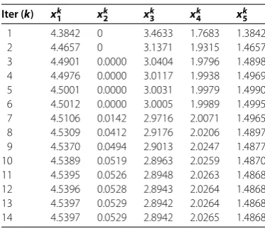
Table 1 Iterations of Scheme (2.1)-(2.3), wherex0= (1, 2, 3, 1, 1)T
Iter (k) xk1 xk2 xk3 xk4 xk5
1 4.3842 0 3.4633 1.7683 1.3842
2 4.4657 0 3.1371 1.9315 1.4657
3 4.4901 0.0000 3.0404 1.9796 1.4898
4 4.4976 0.0000 3.0117 1.9938 1.4969
5 4.5001 0.0000 3.0031 1.9979 1.4990
6 4.5012 0.0000 3.0005 1.9989 1.4995
7 4.5106 0.0142 2.9716 2.0071 1.4965
8 4.5309 0.0412 2.9176 2.0206 1.4897
9 4.5370 0.0494 2.9013 2.0247 1.4877
10 4.5389 0.0519 2.8963 2.0259 1.4870
11 4.5395 0.0526 2.8948 2.0263 1.4868
12 4.5396 0.0528 2.8943 2.0264 1.4868
13 4.5397 0.0529 2.8942 2.0264 1.4868
14 4.5397 0.0529 2.8942 2.0265 1.4868
Table 2 With the tolerance= 10–6
Scheme (2.1)-(2.3) Algorithm 2a in [14]
Problem No. iterations CPU times (seconds) Problem No. iterations CPU times (seconds)
1 16 1.8438 1 23 1.1388
2 13 1.4375 2 15 2.1103
3 19 2.5156 3 25 3.1023
4 21 2.7031 4 22 3.7801
5 14 1.7344 5 17 2.0183
6 16 1.9531 6 19 2.0081
7 16 1.8594 7 21 1.5921
8 19 2.5938 8 25 3.0142
9 16 2.1875 9 15 1.9082
10 12 1.5632 10 23 4.0115
Subproblems (.) and (.) can then be solved efficiently, for example, by the Matlab optimization toolbox. Lemma . shows that ifr(xk) = , thenxkis a solution to problems
EP(f,C). So, we can say thatxkis an-solution to problemsEP(f,C) if we have r(xk) ≤ with> . Taking= –,γ = .,β= andσ= , we obtained the iterates in Table .
The approximate solution obtained after iterations is
x= (., ., ., ., .)T.
In Table , we compare Scheme (.)-(.) with Algorithm a in []. Now, there have been some changes in this case: M,Band the first component of vector qare
cho-sen randomly in (, ), and the first component of vectordis chosen randomly in (, ). In both cases, we use Algorithm a with the same equilibrium bifunction, the quadratic regularization functionG(x) :=ln( + x) and parametersθ= .,ρ= ,α= ..
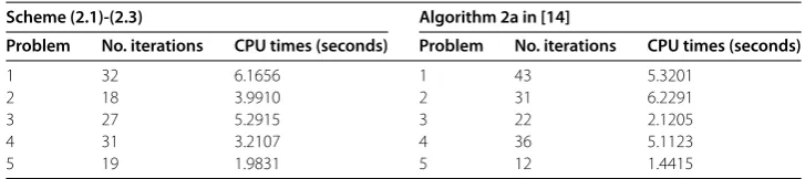
Case . We use Scheme (.)-(.) with the same equilibrium problems and dates as in Case . Unless the bifunctionF(x,y) :=M(x+y) +D(x+y) +q, whereDis defined by the components of theD(x), isDj(x) =djarctan(xj)∀j= , . . . , ,dj is chosen by d= (, , , , )T. This example is given by Bnouhachem (see []). Under these assumptions, it can be proved thatf is continuous and pseudomonotone onC.
We also see that in Step the solutionykcan be written by
yk:=arg minMxk+y+Dxk+y+q,y–xk+
βx–x
k
|x∈C
[image:14.595.118.476.288.418.2]
Table 3 With the tolerance= 10–6
Scheme (2.1)-(2.3) Algorithm 2a in [14]
Problem No. iterations CPU times (seconds) Problem No. iterations CPU times (seconds)
1 32 6.1656 1 43 5.3201
2 18 3.9910 2 31 6.2291
3 27 5.2915 3 22 2.1205
4 31 3.2107 4 36 5.1123
5 19 1.9831 5 12 1.4415
where
Dxk+y=darctan
xk+y
, . . . ,darctan
xk+y T
,
and in Step ,
∂f
zk,zk=Fzk,zk
=Mzk+darctan
zk, . . . ,darctan
zkT+q.
Thus, the sequence{wk}is uniform bounded. There have been some changes in this case: f(x,y) =M(x+y) +D(x+y) +q,y–x, whereD(x) = (darctan(x), . . . ,darctan(x))T, butd
is defined, the components are chosen randomly in (, ). Choosingγ = .,β= ,σ= . andx¯= (, , , , )T∈Cand comparing Scheme (.)-(.) and Algorithm . in [], we obtained the computation presented in Table .
We perform Scheme (.)-(.) and Algorithm a [] in Matlab Ra running on a PC Desktop Intel(R) Core(TM) Duo CPU T@ .GHz . GB, Gb RAM.
Competing interests
The authors declare that they have no competing interests.
Authors’ contributions
The main idea of this paper was proposed by PNA. PNA, JKK and NDH prepared the manuscript initially and performed all the steps of the proof in this research. All authors read and approved the final manuscript.
Author details
1Department of Scientific Fundamentals, Posts and Telecommunications Institute of Technology, Hanoi, Vietnam. 2Department of Mathematics Education, Kyungnam University, Masan, Kyungnam 631-701, Korea.3Department of
Natural Sciences, Duy Tan University, Danang, Vietnam.
Acknowledgements
We are very grateful to the anonymous referees for their really helpful and constructive comments on improving the paper. This work was completed while the first author was studying at the Kyungnam University for the NRF Postdoctoral Fellowship for Foreign Researchers. And the second author was supported by the Basic Science Research Program through the National Research Foundation of Korea (NRF) funded by the Ministry of Education, Science and Technology (2012R1A1A2042138).
Received: 12 September 2012 Accepted: 19 November 2012 Published: 7 December 2012 References
1. Blum, E, Oettli, W: From optimization and variational inequality to equilibrium problems. Math. Stud.63, 127-149 (1994)
2. Daniele, P, Giannessi, F, Maugeri, A: Equilibrium Problems and Variational Models. Kluwer Academic, Dordrecht (2003) 3. Hai, NX, Khanh, PQ: Existence of solutions to general quasi-equilibrium problems and applications. J. Optim. Theory
Appl.133, 317-327 (2007)
4. Konnov, IV: Application of the proximal point method to nonmonotone equilibrium problems. J. Optim. Theory Appl.
119, 317-333 (2003)
6. Anh, PN, Kim, JK: Outer approximation algorithms for pseudomonotone equilibrium problems. Comput. Math. Appl.
61, 2588-2595 (2011)
7. Anh, LQ, Khanh, PQ: Existence conditions in symmetric multivalued vector quasi-equilibrium problems. Control Cybern.36, 519-530 (2007)
8. Mastroeni, G: Gap function for equilibrium problems. J. Glob. Optim.27, 411-426 (2004)
9. Moudafi, A: Proximal point algorithm extended to equilibrium problem. J. Nat. Geom.15, 91-100 (1999) 10. Noor, MA: Auxiliary principle technique for equilibrium problems. J. Optim. Theory Appl.122, 371-386 (2004) 11. Quoc, TD, Anh, PN, Muu, LD: Dual extragradient algorithms to equilibrium problems. J. Glob. Optim.52, 139-159
(2012)
12. Facchinei, F, Pang, JS: Finite-Dimensional Variational Inequalities and Complementary Problems. Springer, New York (2003)
13. Konnov, IV: Combined Relaxation Methods for Variational Inequalities. Springer, Berlin (2000)
14. Tran, DQ, Dung, ML, Nguyen, VH: Extragradient algorithms extended to equilibrium problems. Optimization57, 749-776 (2008)
15. Anh, PN: An LQP regularization method for equilibrium problems on polyhedral. Vietnam J. Math.36, 209-228 (2008) 16. Auslender, A, Teboulle, M, Ben-Tiba, S: A logarithmic-quadratic proximal method for variational inequalities. Comput.
Optim. Appl.12, 31-40 (1999)
17. Bnouhachem, A: An LQP method for pseudomonotone variational inequalities. J. Glob. Optim.36, 351-363 (2006) 18. Solodov, MV, Svaiter, BF: A new projection method for variational inequality problems. SIAM J. Control Optim.37,
765-776 (1999)
19. Anh, PN: Strong convergence theorems for nonexpansive mappings and Ky Fan inequalities. J. Optim. Theory Appl. (2012). doi:10.1007/s10957-012-0005-x
20. Anh, PN, Kuno, T: A cutting hyperplane method for generalized monotone nonlipschitzian multivalued variational inequalities. In: Bock, HG, Phu, HX, Rannacher, R, Schloder, JP (eds.) Modeling, Simulation and Optimization of Complex Processes. Springer, Berlin (2012)
21. Muu, LD, Nguyen, VH, Quy, NV: On Nash-Cournot oligopolistic market equilibrium models with concave cost functions. J. Glob. Optim.41, 351-364 (2008)
22. Anh, PN, Muu, LD, Strodiot, JJ: Generalized projection method for non-Lipschitz multivalued monotone variational inequalities. Acta Math. Vietnam.34, 67-79 (2009)
23. Takahashi, S, Toyoda, M: Weakly convergence theorems for nonexpansive mappings and monotone mappings. J. Optim. Theory Appl.118, 417-428 (2003)
24. Anh, PN: A hybrid extragradient method extended to fixed point problems and equilibrium problems. Optimization (2012). doi:10.1080/02331934.2011.607497
25. Anh, PN, Muu, LD, Nguyen, VH, Strodiot, JJ: Using the Banach contraction principle to implement the proximal point method for multivalued monotone variational inequalities. J. Optim. Theory Appl.124, 285-306 (2005)
26. Dafermos, S: Exchange price equilibria and variational inequalities. Math. Program.46, 391-402 (1990)
doi:10.1186/1029-242X-2012-288