AN ALGORITHM FOR FAIRNESS BETWEEN SECONDARY
USERS IN COGNITIVE RADIO NETWORK
1ABDELLAH IDRISSI, 2SAID LAKHAL
Research Computer Sciences Laboratory (LRI) Computer Sciences Department, Faculty of Sciences
University Mohammed V - Agdal, Rabat
E-mail: 1 [email protected], 2 [email protected]
ABSTRACT
Scheduling Secondary Users (SUs), to exploit the free channels in Cognitive Radio Network, represents one of the major challenges. In this work we propose an algorithm to ensure fairness of service between the secondary users. This fairness is expressed in terms of transfer rates. The algorithm produces a chain containing the order wherein the packets of each SU will be sent. The experimental results provide transfer rates too close to their average. This proves the efficiency of scheduler proposed.
Keywords: Cognitive Radio, Scheduling, Fairness, Standard Deviation.
1. INTRODUCTION
Cognitive Radio Networks (CRN) is an area of research booming. It was initiated by Mitola in [1]. The author has dealt with the problems related specially to the spectra. After the emergence of this field, several areas of research including Artificial Intelligence and Telecommunications... have addressed the issue. Current challenges for the researchers focus on the scarce resources (like spectrum, energy, time and space) and the increasing demands, particularly from secondary users, on unused frequencies. This raises the question of a possible saturation of these frequency bands.
Scheduling in the CRN consists to assign the free channels for SUs so they can transfer their data packets. To do this, we must determine, during a fraction of time, some parameters like free frequencies, the state of the queue of each SU and the procedure for channel allocation.
To achieve these goals, we believe it would be interesting to develop an efficient scheduler to properly control CRN. Our work focuses on a CRN composed of several SUs, only one channel and only one PU.
To obtain Transfer Rate (TR) almost identical between all SUs, we have grouped the SUs which admit the same number of packets to be transmitted in the same group. The proposed method allows placing the Group which has More Packets (GMP) at the end of the Scheduling Chain (SC). Thus, at each iteration of our algorithm, there will be a new GMP.
The algorithm stops when all the packets are transmitted. The effectiveness of the algorithm is proved by the value of the Standard Deviation between the TR (SDTR). Thus, in all this work, the value of SDTR is always less than 1. We expose in the next section, some previous work. In section 3, we present a CRN constituted by only one channel, one PU and several SUs. We propose a problem modeling in section 4 and expose our algorithm in section 5. In section 6, we develop some applications and finally we conclude in section 7.
2. RELATED WORKS
There are several studies in the literature which deal with this area of scheduling the users in Cognitive Radio Network like [1, 2, 3, 4, 5, 6]. In [2], the authors treated maximizing the sum of the capacity of the SUs, the stability of the queue of each SU and the equation which characterizes the transmission of the data packets. However, the authors have not given particular attention to equality between the SUs. In their approach, there is no organization of SUs relatively to the number of packets which they have to send.
In [4], the authors proposed a scheduling scheme opportunistic for spectrum. In order to maximize the transfer rate, the proposed algorithm estimates the number of packets sent by each SU through each channel. But they did not address the fairness between SUs.
In [5], the authors have analyzed a cognitive radio network in which several SUs can share the same spectrum, and also one SU can use multiple spectra simultaneously in order to transmit its data. The authors seek to determine the optimal energy distribution rate for each SU in order to achieve fairness between SUs. Their approach takes into account the history of user activities to meet the QoS. To quantify the activity, they introduced the concept of dynamic weight for each SU.
In [6], the authors have used a hybrid system, to improve the performance of the SU and increase their chances of access to spectrum. They analyzed the queues of the users to show the influence of the PU on the performance of the SU.
The Performance in CRN is measured in terms of:
– Quality of Service for PU: The SU can access the spectrum only when it is not used by PU. Also, SU must leave the spectrum when a PU asks for it [6, 7]. It is necessary to avoid collision problem between users.
– Transfer rate of SUs: the SUs should send much data. In fact, The CRN that can reach a very high level is considered more effective [8, 9, 10, 11]. – Operating spectra: The exploitation of spectrum by SUs should be maximum [12, 13].
– Interference: Interference decreases the quality of service on a network. In a CRN, it is necessary to reduce interference to a minimum [14, 15].
[image:2.612.311.501.199.286.2]– Energy: It is one of the most limited resources. It must be managed properly to ensure maximum service to users while consuming minimal energy [16, 17].
Our study is based on the principle of fairness between SUs. We consider that the size of the queue is an important property. For this reason, we grouped the SUs according to this property in order to transmit together their packets of data. Thus, the SUs with queues having the same size will be treated in the same way. Equity is expressed in terms of transfer rate. Our contributions include: – Ensure the quality of services (QoS) for the PU, since the SUs operate only when the channel is free and they leave it as soon as one PU asks for it [1, 4], – Study the problem of fairness of service between SUs, considering the combination of SUs depending on the number of packets to be transmitted, and
– Propose a scheduling algorithm that reduces the Standard Deviation of the Transfer Rate (SDTR).
3. CRN WITH A SINGLE CHANNEL, A SINGLE PU AND SEVERAL SUs
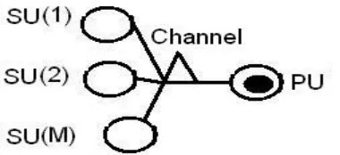
Figure 1 shows a CRN with a single channel, a single PU and several SUs.
Figure 1: CRN with a single channel, a single PU and several SUs.
All our work is based on the following hypothesis: The scheduler knows the states of channel for an Allocation Interval (AI).
3.1 Allocation Intervals (AI)
[image:2.612.310.517.422.486.2]We determine the state of the channel during the AI where AI = [kT, (k + 1)T] (Figure 2).
Figure 2: Allocation Interval (AI)
To specify the channel state for an AI, we introduced the notion of Indivisible Interval (II). So, we consider that the Allocation Interval (AI) can be divided into q Indivisible Intervals (II) each of which is identified by:
)
1
(
)]
1
(
,
[
+
+
+
=
h
q
T
kT
h
q
T
kT
I
hkWhere
h
∈
{
0
,...
...,
q
−
1
}
For
I
hk,
the channel can take one of the two states: free or busy [2].Let C be the channel capacity. The amount of
information carried by the channel for
I
hk is given by equation (2).)
2
(
*
To facilitate the study, we assume Q as a measurement unit. Thus, we consider that each packet has a size Q. The amount of information of SU(m) can be given by equation (3):
)
3
(
*
mm
Q
n
Q
=
where
n
m is the number of packets that SU(m) are looking to send.For each SU, we compute the amount of information using equation (3), and then we proceed to grouping the SUs according to the number of data packets.
3.2 Organization of SUs
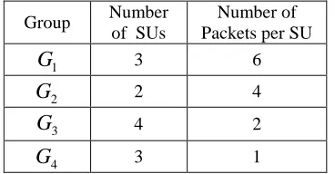
[image:3.612.105.289.484.580.2]The SUs with the same number of packets are assembled in the same group (see an example in Figure 3).
Figure 3: Grouping the SUs according to the number of packets.
The table 1 below summarizes Figure 3.
Table 1. Grouping the SUs according to the number of packet (Figure 3).
Group Number of SUs
Number of Packets per SU
1
G
3 62
G
2 43
G
4 24
G
3 1The groups failing to transmit all their packets during an Allocation Interval (AI) must wait the next AI. This process is repeated until all the packets will be sent.
In the proposed approach, we consider all these intervals as a single unit. We assume also that two successive packets of the same group can be sent at different AIs. The packets that are on the same line of a given group will be sent successively and without interruption.
We will focus only on packet transmission regardless of the AI used.
We model the problem in the following section. For this, we need to define some parameters.
4. SYSTEM MODEL
Let us note:
-
R
is
the number of groups.-
G
iis
a group containingp
i SUs.-
SU
i,mis
a SU identified by its groupG
iand its index m.
-
EverySU
i,m hasp
i packets to transmit.-
AR
iis the Achievement Rate of service for the groupG
ii.e.
AR
i is the number of fractions and the free time necessary to perform the service ofG
i.-
AR
the vector carrying the service:[
]
TR
AR
AR
AR
=
1,...,
We will formulate the problem based on the criterion of fairness of service between SUs in the following paragraph.
4.1. Problem Formulation
4.1.1. Minimization of the difference between the transfer rates
We consider that in order to serve in the same way all SUs, we must reduce the difference between the transfer rates to the minimum possible.
Assuming that
G
i hasg
i SUs and every SU hasp
i packets to be transmitted. Thus, this group hasi i
g
p
packets. IfAR
iis the Achievement Rate of service for the groupG
i andi
fr
i is the transfer rate of the groupG
i, then we will have:)
4
(
i i i i
AR
g
p
r
=
{
1
,...,
}
(
5
)
,
j
R
i
r
r
i−
j∀
∈
The Group
G
i sends all its packets after using a number of free fractions greater thanp
ig
i. To not monopolize the service, the groupG
i must wait other groups to send their packets.So, we can write:
)
6
(
, 1∑
= ≠ =+
=
j Ri j j j ij i i
i
p
g
g
AR
α
Let
α
ijg
jbe the number of packets ofG
jto send before thanG
icompletes its service. So, we will haveα
ij≤
p
j.If we replace in (4)
AR
i by its value in (6), we obtain:)
7
(
1
1
, 1 , 1∑
∑
= ≠ = = ≠ =+
=
+
=
j Ri j j i i
j ij R j i j j j ij i i i i i
g
p
g
g
g
p
g
p
r
α
α
Note that:
0
<
r
i≤
1
.
The problem can be written as follows:
{
}
≤
≤
∈
−
=
j ij j ip
SC
R
j
i
r
r
Min
PB
α
0
,...,
1
)
,
(
2 1
In PB1, we have
2 ) 1 (R−
R objective functions to
minimize. We seek to reformulate (PB1) in order to
reduce it to a problem with only one objective function.
4.1.2. Reformulation of PB1
Let
r
*be a solution of PB1, then:{
1
,....,
}
(
8
)
,
,
2 * *R
j
i
r
r
r
r
i−
j≤
i−
j∀
∈
The formula (8) implies:
{
1
,..,
}
(
9
)
,
,
2 ) , ( ) 1 , 1 ( 2 ) , ( ) 1 , 1 ( 2 * *R
j
i
r
r
r
r
R R j i R R ji
−
≤
∑
−
∀
∈
∑
If we consider the following problem PB2:
≤
≤
−
=
∑
j ij R R j ip
SC
r
r
Min
PB
α
0
,
)
(
) , ( ) 1 , 1 ( 2 2From the formula (9), it is easy to deduce that any solution of PB1 is also a solution of PB2. So to solve
PB1, it suffices to solve PB2, and test the obtained
solutions on the problem PB1.
The solution of PB2 is a vector with components
which are very close. Therefore, they are also very close to their average.
Let r be the average of
r
i,
i
∈
{
1
,...,
R
}
and)
(
r
σ
the standard deviation ofr
i. Following [8], we can write:∑
==
R i ir
R
r
1)
10
(
1
)
11
(
)
(
1
)
(
1 2∑
=−
=
R i ir
r
R
r
σ
The problem can be written as follow:
≤
≤
=
j ijp
SC
r
Min
PB
α
σ
0
)
(
3The resolution of the problem PB3 must consider
two conditions:
1) Optimization: to minimize the objective function. 2) Scheduling: to determine the order in which packets will be sent.
The Mathematical solving of the problem PB3
allows to determine easily the values of
α
ij,
for
(
i
,
j
)
∈
{
1
,...,
R
}
2. But in this case, we have no information about the order in which packets will be sent. Also, if we apply the scheduling we may lose the control of the optimization.To deal with these shortcomings, we propose in the next section an algorithm taking into account simultaneously the constraints of scheduling and the constraints of optimization. Before that, we construct a Scheduling Chain (SC).
5. ALGORITHM
The algorithm is a function of two arguments:
P: a column vector composed of three lines containing the number of packets for SU of the same group.
This function returns the Chain as a result.
ALGORITHM Mono_ Scheduler (G, P)
BEGIN
1 GP [G, P] 1 2 GP1 Sort(GP)2 3 [G1, P1] GP1 4 Chain empty chain 5 St [G1, P1, G1*P1] 6 [u, v, w] St 7 while
v
≠
0
do8 T Max(w)3
9 s NumberOfLines(T) 10 if
s
≥
2
then11 for o=1 to s 12 g T(o, 1)
13 ChainAddChain(g, 1)4 14 St(g, 2) St(g, 2)-1 15 St(g, 3) St(g, 2)*St(g, 1) 16 end for
17 else
18 v1 FirstFollowingIndex(w)5 19 g T(1, 1)
20 if
v
1(
1
,
1
)
≠
0
then21 z (T(1, 2)-v1(1, 3))/u(g) 22 en IntegerPartAdd1(z)6 23 else
24 en T(1, 2) 25 end if
26 ChainAddChain(g, en) 27 St(g, 2) St(g, 2)-en 28 St(g, 3) St(g, 2)*St(g, 1) 29 end if
30 [u, v, w] St 31 end while
32 reverse(Chain)7
END
The Scheduling Chain (SC) is formed by couples. The first component of each couple is the group number and the second component is the number of packets to send. Then, after computing the number of packets of each group, we place the one which has the most packets at the end of the SC.
1Concatenation of G and P.
2Sort the components of P in descending order and put the result
in GP1.
3Maximum components w.
4Add the pair (g, 1) to the chain.
5The second value of w that just happens after Max (w), it is
accompanied by its index.
6Integer part add 1.
7
Start with the last element and return to the first
We also compute the number of packets that this group will keep and then we subtract this number of packets kept in order to permit to another group having more packets to transmit its packets. We repeat the procedure until all the packets will be sent.
The proposed algorithm allows establishing the SC that can be exploited to compute the rate, the inverse of transfer rate and the SDIR.
6. APPLICATIONS
We applied our algorithm on several instances which are randomly generated. We will show here only two instances.
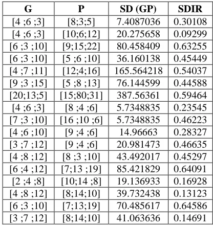
Instance 1: Three groups and 17 samples (table 2). The table contains four columns:
[image:5.612.89.262.168.559.2]1st column: Vector G 2nd column: Vector P 3rd column: SD(P*G) 4th column: SDIR
Table 2: This table shows the values for SD(GP) and for SDIR.
G P SD (GP) SDIR
[4 ;6 ;3] [8;3;5] 7.4087036 0.30108 [4 ;6 ;3] [10;6;12] 20.275658 0.09299 [6 ;3 ;10] [9;15;22] 80.458409 0.63255 [6 ;3 ;10] [5 ;6 ;10] 36.160138 0.45449 [4 ;7 ;11] [12;4;16] 165.564218 0.54037 [9 ;3 ;15] [5 ;8 ;13] 76.144599 0.44588 [20;13;5] [15;80;31] 387.56361 0.59464 [4 ;6 ;3] [8 ;4 ;6] 5.7348835 0.23545 [7 ;3 ;10] [16 ;10 ;6] 5.7348835 0.46223 [4 ;6 ;10] [9 ;4 ;6] 14.96663 0.28327 [3 ;7 ;12] [9 ;4 ;6] 20.981473 0.46635 [4 ;8 ;12] [8 ;3 ;10] 43.492017 0.45297 [6 ;4 ;12] [7;13 ;19] 85.421829 0.64091 [2 ;4 ;8] [10;14 ;8] 19.136933 0.16928 [4 ;8 ;12] [8;14;10] 39.732438 0.13123 [6 ;3 ;10] [7;13;19] 70.485617 0.64586 [3 ;7 ;12] [8;14;10] 41.063636 0.14691
The outcomes of interest are those of the third and fourth column. The components of SR (GP) will be sorted in descending in order to facilitate the graphical representation.
Table 3: Values for SD(GP) and SDIR.
SD(GP) SDIR
[image:5.612.308.516.375.596.2]70.485617 0.64586 65.564218 0.54037 43.492017 0.45297 41.063636 0.14691 39.732438 0.13123 36.160138 0.45449 33.875589 0.46223 20.981473 0.466351 20.275658 0.09299 19.136933 0.16928 14.96663 0.28327 7.40870 0.30108 5.73488 0.23545
Instance 2: Five groups and 13 samples. In this case, we have a large table. It is divided into two tables: Table 4 (Containing the vector G and P) and table 5 (containing SD(GP) and SDIR).
Table 4: This table shows the values for G and P.
[image:6.612.95.483.71.272.2] [image:6.612.317.514.394.565.2]G P
[5;9;3,9;14] [15;4;8;10;20] [15;8;6;4;10] [8;23;11;4;33]
[image:6.612.136.264.522.695.2][15;5;7;18;10] [9;22;9;18;14] [17;11;38;16;8] [12;16;5;30;2] [18;23;19;24;13] [13;27;16;33;9] [25 ;9 ;17 ;14 ;7] [24;8;13;21;12] [8;12;14;25;21] [6;17;16;23;5] [15;19;13;24 ;5] [14;18;20;30;11] [18;12;11;24;15] [16;10;12;2;7] [12;17;13;21;15] [8;14;13;23;6] [5;9;3;14;10] [4 ;8 ;10;20;15] [12;17;10;21;15] [18;14;13;23 ;6] [5 ;5 ;17 ;18 ;10] [9;20;19;18;14]
Table 5: Values for SD(GP) and for SDIR.
SD(GP) SDIR
92.7275 0.83 108.845 0.65 89.0765 0.82 149.7176 0.94 252.3652 0.80 192.0566 0.88 183.564 0.78 221.979 0.75 80.0589 0.71 144.398 0.90 96.3775 0.82 137.010 0.80 115.935 0.64
Sorting SD(GP), in descending order gives:
Table 6: Values for SD(GP) and for SDIR.
SD(GP) SDIR
252.36529 0.8052531 221.97982 0.7593584 192.05666 0.8871719 183.56405 0.78738 149.7176 0.9469645 144.39861 0.9068629 137.01036 0.8085614 115.9355 0.6487722 108.84558 0.6595745 96.377591 0.8279039 92.727558 0.8355148 89.076596 0.8275135 80.058978 0.7101899
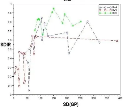
The execution of the algorithm on different examples shows that the value of SDIR is always less than 1 (see Figure 4).
Figure 4 summarizes the previous results. The components of SD(GP) are represented on the x-axis and the components of SDIR are represented on the y-axis.
Figure 4: SDIR In terms of SD(GP)
We notice that for different values of R, there is always SDIR < 1. This shows that
i
r
1 is too close to
their average. This result holds even for large values of SD(GP).
7. CONCLUSION
results show that the standard deviation of the inverse transfer rate is always less than 1.
This is valid even for groups with numbers of packets widely dispersed around their average. Our algorithm is general and can be adapted to any similar problem.
REFERENCES
[1] Mitola J., "Cognitive radio: an integrated agent architecture for software defined radio", Ph.D. Dissertation. Royal Institute of Technology (KTH). Teleinformatics. Electrum 204. SE-164 40 Kista. Sweden. 8 May 2000.
[2] Rahul Urgaonkar and Michael J. Neely. “Opportunistic Scheduling with Reliability Guarantees in Cognitive Radio Networks", In IEEE TRANSACTIONS ON MOBILE COMPUTING, Vol. 8, N°. 6, June 2009, pp. 766-777.
[3] Ho ting Cheng and Weihua Zhuang, "Simple channel sensing order in cognitive radio networks". In IEEE Journal on Selected Areas in Communications. Volume 29, Issue 4. April 2011. pp. 676 – 688.
[4] Bassem Zayen, Majed Haddad, Awatif Hayar and Geir E. Ien, "Binary power allocation for cognitive radio networks with centralized and distributed user selection strategies" In Elsevier journal Physical Communication. Vol. 1. Issue 3. September 2008. pp. 183-193.
[5] Lutfa Akter and Balasubramaniam Natarajan, "Modeling Fairness in Resource Allocation for Secondary Users in a Competitive Cognitive Radio Network", in proceeding of Wireless Telecommunications Symposium (WTS), 21-23 April 2010, pp. 1-6.
[6] Jie Hu, Lie- Liang Yang, Lajos Hanzo. “Optimal Queue Scheduling for Hybrid Cognitive Radio Maintaining Maximum Average Service Rate Under Delay Constraints”. In IEEE Global Communications Conference. 3-7 Dec. 2012. pp. 1398 - 1403. Anaheim, CA.
[7] Ashwini Kumar , Kang G. Shin, Jianfeng Wang and Kiran Challapali "A Case Study of QoS Provisioning in TV-band Cognitive Radio Networks". In proceedings of 18th International Conference on Computer Communications and Networks. ICCCN 2009. pp. 1-6.
[8] Chandrasekharan Raman, Jasvinder Singh, Roy D. Yates and Narayan B. Mandayam. "Scheduling in Cognitive Networks: Scheduling Variable Rate Links- Centralized and Decentralized approaches", Chapter 15 in Book “Cognitive Wireless Networks”. Editors Frank
H. P. Fitzek & Marcos D. Katz. Springer 2007, pp. 285-305.
[9] Chandrasekharan Raman. "Relaying and Scheduling in Interference Limited Wireless Networks", Ph.D. Collection Graduate School - New Brunswick. Rutgers, The State University of New Jersey. May 2010
[10] Shuang Li, Zizhan Zheng, Eylem Ekici and Ness B. Shroff. "Maximizing System throughput Using Cooperative Sensing in Multi-channel Cognitive Radio Networks", http://arxiv.org/abs/1111.3041 November 13, 2011.
[11] Shuang Li, Zizhan Zheng, Eylem Ekici and Ness Shroff. "Maximizing System Throughput by Cooperative Sensing in Cognitive Radio Networks", arXiv.org > cs > arXiv:1211.3666, November 15, 2012.
[12] Zhu Ji and K. J. Ray Liu, "Dynamic Spectrum Sharing: A Game Theoretical Overview",IEEE Communications Magazine, May 2007, pp. 88-94.
[13] Jamal Elhachmi and Zouhair Guenoun. "Frequency Assignment for Cellular Mobile systems using a Hybrid Tabu search", Multimedia Computing and Systems (ICMCS), 7-9 April 2011. pp. 1 - 5
[14] Yangyang Li "Cognitive Interference Mangement in 4G Autonomous Femtocells". Thesis. Department of Electrical and Computer Engineering University of Toronto, 2010. published in: http://hdl.handle.net/1807/24815. [15] Abdoulaye Zana BAGAYOKO "Spectrum
Sharing under interfering Constraints", Ph.D. Thesis presented at University of Cergy-Pontoise. Defended on Octobre 29, 2010.
[16] Zaheer Khan "Coordination and adaptation techniques for efficient resource utilization in cognitive radio networks" Academic dissertation presented at the Faculty of Technology of the University of Oulu, on 18 November 2011. [17] Moshe Masonta, Yoram Haddad, Luca De