A NEURAL NETWORK-BASED SVPWM CONTROLLER FOR
A TWO-LEVEL VOLTAGE-FED INVERTER INDUCTION
MOTOR DRIVE
1AHMED A. HASSAN, 2SAMIR DEGHEDIE, 3MOHAMED EL HABROUK
1, 2, 3
Department of Electrical Engineering, Faculty of Engineering, Alexandria University
E-mail [email protected], [email protected]
,
[email protected]ABSTRACT
In this paper, a detailed description of a neural network-based implementation of the SVPWM algorithm for two-level voltage source inverters is proposed using a modular approach which facilitates the expansion of the scheme to higher levels SVM, each step in the SVPWM algorithm is achieved using a simple feed-forward artificial neural network that consists of one or more layers. Simulation results are provided by employing the proposed scheme inside a closed loop V/Hz drive system.
Keywords: Space Vector Modulation (SVM), Artificial Neural Networks (ANNs), Two-Level Inverter
1. INTRODUCTION
The main objective of inverters is to produce an AC output waveform from a DC power supply where the amplitude, phase, and frequency of the voltage should always be controllable which is a requirement for many applications such as adjustable speed drives (ASDs), uninterruptible power supplies (UPS), active filters, etc [1]
Modulation techniques are responsible for controlling the amount of time and the sequence used to switch the power switches on and off. The modulation techniques most used are the sinusoidal pulse-width modulation (SPWM), space-vector modulation (SVM) and the selective harmonic elimination pulse-width modulation (SHEPWM) [1].
The square-wave or six-step operation mode of the inverter is simple to implement and characterized by low switching losses because there are only six switching per cycle of the fundamental frequency. Unfortunately, the lower order harmonics will cause large distortions of the current wave unless filtered by a bulky low-pass filter [2].
2. FUNDAMENTALS OF SVM
Space-vector pulse-width modulation has recently grown as a very popular PWM method for voltage-fed converter AC drives [3]. SVM is based on the representation of the three phase quantities as vectors in a two-dimensional α-β plane [4].
2.1 Inverter Topology and Space Vectors The two-Level three-phase (VSI) is shown in figure 1. Valid switch states for the two-level three-phase VSI are shown in table 1, States 1 - 6 produce non-zero ac output voltages while states 0 & 7 produce zero ac line voltages. In this case, the ac line currents freewheel through either the upper or lower components [2].
The selection of the states in order to generate the given waveform is done by the modulating technique that should ensure the use of only the valid states [1]. A “0” denotes that the lower switch is conducting while a “1” denotes that the upper switch is conducting in the respective leg
Vdc
S1 S3 S5
S2
S6
S4
D1 D3 D5
D2
D6
D4
N A
[image:1.612.323.501.527.639.2]B C
Table 1: Valid Switch States for Two-Level Inverter
2.2 Rotating Space Vector and SVM Theory [2] If the three-phase sinusoidal and balanced voltages with peak value Vm are given by:
va= Vmcos(θ) (1)
vb= Vmcos�θ −2π
3� (2)
vc= Vmcos�θ+2π
3� (3)
The space vector in complex notation is given by:
V�=2
3�va+ vbej2π 3⁄ + vce−j2π 3⁄ � (4)
Substituting equations (1), (2) and (3) into equation (4) and simplifying, we get:
V� = Vmejθ= Vmejωt (5)
This indicates that the vector 𝐕� rotates in circular orbit with angular velocity ω, where the direction of rotation depends on the phase sequence of the voltages . The vector magnitude is given by:
|V�| = Vm = �vα2+ vβ2 (6)
At any instant, the vector angle 𝜽w.r.t the α-axis is given by
θ = tan−1 vβ
vα (7)
If the reference vector V�∗ lies in sector 1 as shown in figure 2, the PWM output is generated by resolving V�∗ using the adjacent vectors V�1&V�2 on a part-time basis to satisfy the average output demand.
Va= 2
√3V∗sin� π
3− θ� (8)
Vb= 2
√3V∗sinθ (9)
[image:2.612.321.509.155.381.2]Where Va and Vbare the components of V�∗aligned in the directions of V�1 & V�2 respectively.
Figure 2: Reference Vector Trajectory and Space Vectors
3. ANN-BASED TWO-LEVEL SVM
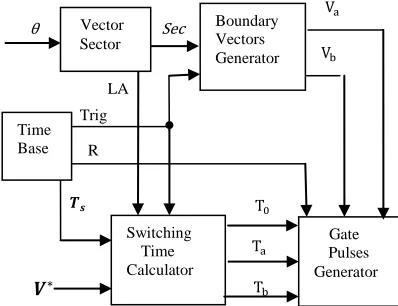
Figure 3 shows the general block diagram for generating the gate pulses for two-level SVM. Each block is responsible for achieving certain task which is described in the following sections.
Figure 3: Block Diagram of Two-Level SVM Generator
3.1 Time Base
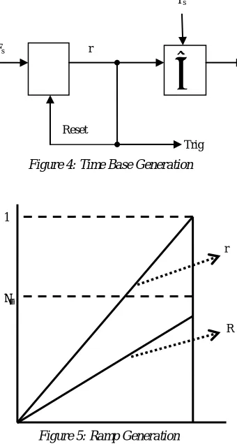
The purpose of the block diagram shown in figure 4 is to generate different timing signals as follows:
The sampling frequency is integrated to produce a ramp function, when the ramp reaches its peak
State “ON” Switches Space Vector
0 S2, S4, S6 V0(000)
1 S1, S2, S6 V1(100)
2 S1, S2, S3 V2(110)
3 S2, S3, S4 V3(010)
4 S3, S4, S5 V4(011)
5 S4, S5, S6 V5(001)
6 S1, S5, S6 V6(101)
7 S1, S3, S5 V7(111)
𝑻𝒔
θ
Vb
Sec Va
T0
Ta
Tb Boundary Vectors Generator
Gate Pulses Generator Switching
Time Calculator Trig
R
𝑽∗
Reference Vector Trajectory
Reference Vector Limit
Time Base
LA Vector Sector
α
β
V1 V2
V3
V4
V5 V6
2
3
Va
Vb
1
6
5 4
[image:2.612.317.516.493.646.2]value, the “Trig” signal is generated and the integrator is reset to indicate the start of a new sampling period. The sampling period “Ts” is generated from the sampling frequency.
Where, Ts = 1
Fs (10)
[image:3.612.313.512.138.222.2]The ramp “r” directly generated from integrating “Fs” is multiplied by the sampling period “Ts” to generate the ramp function “R” with amplitude equal to “Ts” (figure 5).
Figure 4: Time Base Generation
Figure 5: Ramp Generation
3.2 Vector Sector
The purpose of this block is to determine the location of the reference vector at the start of the sampling period. Figure 6 represents a simplified block diagram for implementing this function.
Where,
Θ Reference vector angle, measured from α- axis Sec Sector number in which the reference vector
Lies at the time of sampling
LA Reference vector Local Angle (measured from The beginning of the sector)
The purpose of generating a local angle is to reflect the equations used to calculate the switching
[image:3.612.106.276.230.548.2]times in sector 1 for all the other sectors without the need to develop separate equations for each sector, figure 7 outlines this concept.
Figure 6 Block Diagram for Determining “Sec” & “LA”
Figure 7 Reference Vector Local Angle (LA)
[image:3.612.313.509.260.405.2]Table 2 shows the relation between “LA” and “θ” indifferent sectors
Table 2: Relation Between “θ”, “LA” and “Sec”
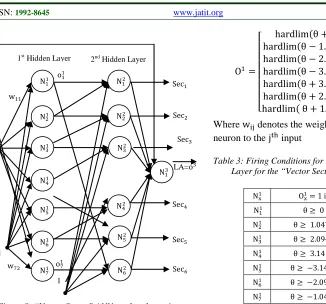
Figure 8 shows the ANN used to generate “Sec” & “LA”.
θ Sec LA
0o <θ < 60o 1 LA = θ
60o < θ < 120o 2 LA = θ - 60o
120o < θ < 180o 3 LA = θ - 120o
-180o< θ < -120o 4 LA = θ + 180o
-120o < θ < -60o 5 LA = θ + 120o
- 60o < θ < 0o 6 LA = θ + 60o
Fs r
Ts
R
Reset
Trig
∫
×
Ts 1
r
R
Θ
Boundary Angles
Sec
LA Compare
Local Angle Calculator
𝑽∗
𝑽∗
LA
[image:3.612.324.509.478.583.2]Figure 8: “Vector Sector” ANN used to determine
Reference Vector Sector “Sec” and Local Angle Inside
Each Sector “LA”
3.2.1 1st Hidden layer:
The purpose of this layer is to indicate (at the sampling instant) that the reference vector angle “θ” is greater than which of the angles that represent the beginning of each sector.
Each neuron in the 1st layer will fire when the reference vector angle “θ” is greater than or equal to the starting angle of the respective sector.
Table 3 shows the firing conditions for neurons of the 1st layer, where, “Nx” is the neuron number and “Ox” is the output of the respective neuron, the superscript denotes the layer number (this convention is followed in all neural networks described throughout this paper).
The weight, input and output matrices are defined as follows:
W1=
⎣ ⎢ ⎢ ⎢ ⎢ ⎢
⎡11 −1.04720
1 −2.0944
1 −3.1416
1 3.1416 1 2.0944 1 1.0472⎦⎥
⎥ ⎥ ⎥ ⎥ ⎤ = ⎣ ⎢ ⎢ ⎢ ⎢ ⎢
⎡ww1121 ww1222
w31 w32
w41 w42
w51 w52
w61 w62
w71 w72⎦
⎥ ⎥ ⎥ ⎥ ⎥ ⎤
P1=�θ
1�
O1=
⎣ ⎢ ⎢ ⎢ ⎢ ⎢ ⎢
⎡hardlim(θ −hardlim(θ1.0472) + 0)
hardlim(θ −2.0944)
hardlim(θ −3.1416)
hardlim(θ+ 3.1416)
hardlim(θ+ 2.0944)
hardlim( θ+ 1.0472) ⎦⎥
⎥ ⎥ ⎥ ⎥ ⎥ ⎤ = ⎣ ⎢ ⎢ ⎢ ⎢ ⎢ ⎢ ⎡o11
o21
o31
o41
o51
o61
o71⎦
⎥ ⎥ ⎥ ⎥ ⎥ ⎥ ⎤
[image:4.612.100.426.69.373.2]Where wij denotes the weight connecting the ith neuron to the jth input
Table 3: Firing Conditions for Neurons of the 1st Layer for the “Vector Sector” ANN
Nx1 Ox1= 1 if
N11 θ ≥ 0
N21 θ ≥ 1.0472 N31 θ ≥ 2.0944 N41 θ ≥ 3.1416 N51 θ ≥−3.1416 N61 θ ≥−2.0944 N71 θ ≥−1.0472
3.2.2 2nd Hidden layer:
This layer indicates that the reference vector angle “θ” is less than which of the angles that represent the end of each sector and to use this information along with the information presented from the 1st layer to determine the boundary angles of the sector in which the reference vector lies. The weight, input and output matrices are defined as follows:
W2=
⎣ ⎢ ⎢ ⎢ ⎢
⎡11 −1−1 −1−1
1 −1 −1
1 −1 −1
1 −1 −1
1 −1 −1⎦⎥
⎥ ⎥ ⎥ ⎤
P2=�O1
1 O 2 1 O 3 1 O 5 1 O 6 1 O 7 1
O21 O13 O41 O16 O71 O11
1 1 1 1 1 1
�
O2=
⎣ ⎢ ⎢ ⎢ ⎢ ⎢
⎡hardlim(O11−O21−1)
hardlim(O12−O31−1)
hardlim(O13−O41−1)
hardlim(O15−O61−1)
hardlim(O16−O71−1)
hardlim(O71−O11−1)⎦
⎥ ⎥ ⎥ ⎥ ⎥ ⎤ = ⎣ ⎢ ⎢ ⎢ ⎢ ⎡sedsec12
sec3
sec4
sec5
sec6⎦
⎥ ⎥ ⎥ ⎥ ⎤ = Sec 1 Sec3 1st Hidden Layer
2nd Hidden Layer
w11
o11
θ
1
w72 o71
Sec1 Sec6 N32 N42 N52 N62 N12 N22 N11 N21 N31 N41 N51 N61 N71 Sec2
LA=o3
Sec4
Which means that neuron 1 will fire and outputs a “1” if O11−O21≥1 which is possible if and only if
O11= 1 AND O12= 0
Therefore, neuron 1 will fire and output a “1” if and only if angle “θ” is greater than 0o but not greater Than 60o, i.e., the reference vector lies in sector 1 The firing conditions for the other neurons can be obtained in a similar manner
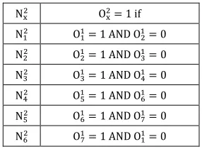
[image:5.612.120.263.241.346.2]The results are summarized in table .4.
Table 4 Firing Conditions for Neurons Of the 2nd Layer
For the “Vector Sector” ANN
Nx2 Ox2= 1 if N12 O11= 1 AND O21= 0 N22 O21= 1 AND O31= 0 N32 O31= 1 AND O41= 0 N42 O51= 1 AND O61= 0 N52 O61= 1 AND O71= 0 N62 O71= 1 AND O11= 0
3.2.3 Output layer
This layer determines the local angle “LA”
The weight, input and output matrices are defined as follows:
W3= [1 0 −1.0472 −2.0944 3.1416
2.0944 1.0472]
P3= [θ O
12 O22 O32 O42 O52 O62]t
O3= [purelin(θ −1.0472O
2
2−2.0944O
3 2 +
3.1416O42+ 2.0944O52+ 1.0472O62)]
only one neuron from the 2nd layer will present a “1” at its output while all other five neurons will present a “0”, indicating the presence of the reference vector in one of six sectors, therefore, all the terms in the expression for O3 will cancel except the first term (𝜽) and only one of the other six terms, consequently, the expression for O3 will always reduce to:
𝑂3=𝐿𝐴=𝜃+𝐶
Where, C is a constant whose possible values are chosen to be multiples of 1.0472 rad (60o) that needs to be subtracted from or added to "θ" to produce “LA” (refer to table 2 & figure 7)
All results are summarized in table 5
Table 5 Results of Output Layer for the “Vector Sector” ANN, Indicating the Expression used to Calculate LA in
Different Sectors
3.3 Switching Time Calculator
This block computes the three time intervals during which the reference vector is sampled to two boundary vectors (V1−V6) and one zero-vector (V0, V7). The “Trig”signal triggers the block to start computing the switching times according to the following equations:
Ta=√3 V∗
VdcTssin�
π
3−LA� (11)
Tb=√3 V∗
VdcTssin(LA) (12)
T0= Ts− Ta− Tb (13)
Where,
Ta Interval of first boundary vector (Va)
Tb Interval of second boundary vector (Vb)
To Interval of zero-vector ( V0, V7)
The non-linear part of equations (11) & (12) which is the “sin” function can be computed using an ANN as shown in figure 9 instead of using look-up tables which requires large memory space.
Figure9:ANN Sine Wave Generator
O12 O22 O32 O42 O52 O62 Sec O3 (LA)
1 0 0 0 0 0 1 θ
0 1 0 0 0 0 2 θ−1.0472
0 0 1 0 0 0 3 θ−2.0944
0 0 0 1 0 0 4 θ+ 3.1416
0 0 0 0 1 0 5 θ+ 2.0944
0 0 0 0 0 1 6 θ+ 1.0472
θ Sin θ
The network is trained using MATLAB Toolbox Neural Fitting Tool (nftool)
3.4 Boundary Vectors Generator
The “Trig” signal initiates the operation of the block to evaluate the two non-zero components of the reference vector "Va" and "Vb" at the start of the sampling period, the input to this block is “Sec” (sector no.) and the outputs are
Va Component of the reference vector aligned
With the start of sector
Vb Component of the reference vector aligned
With the end of sector
Figure 10 shows the neural network used to produce the boundary vectors.
The weight, input and output matrices are defined as follows:
W =
⎣ ⎢ ⎢ ⎢ ⎢
⎡1 1 0 0 0 10 1 1 1 0 0 −0.5−0.5
0 0 0 1 1 1 −0.5
1 0 0 0 1 1 −0.5
1 1 1 0 0 0 −0.5
0 0 1 1 1 0 −0.5⎦⎥
⎥ ⎥ ⎥ ⎤
P =�Sec
1 �=
⎣ ⎢ ⎢ ⎢ ⎢ ⎢ ⎡sedsec12
sec3
sec4
sec5
sec6
1 ⎦⎥ ⎥ ⎥ ⎥ ⎥ ⎤
O = hardlim[WP]
[image:6.612.314.522.301.404.2]1
Figure 10: ANN for producing the Boundary Vectors
The elements of the input matrix, denotes the active sector (this is exactly the output matrix of the 2nd hidden layer from the “Vector Sector” ANN)
. The weight matrix elements are chosen such that the space vectors elements are aligned vertically in the first six columns (each column contains the two vectors that are the boundaries of the six sectors), i.e., the boundary vectors of sector 1 (100 & 110) are aligned in column1while the boundary vectors of sector 2 (110 & 010) are aligned in column 2 and so on.(refer to table 1 and figure 2 for boundary vectors in each sector).
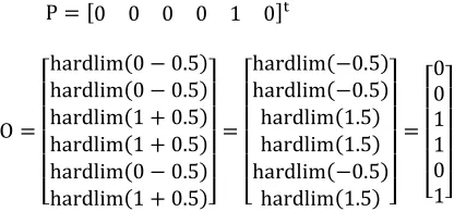
The weight of the bias is chosen so that, the elements of the column which corresponds to the active sector will be available at the output. For example, if the reference vector lies in sector 5, then:
P = [0 0 0 0 1 0]t
O =
⎣ ⎢ ⎢ ⎢ ⎢
⎡hardlim(0hardlim(0−−0.5)0.5) hardlim(1 + 0.5) hardlim(1 + 0.5)
hardlim(0−0.5)
hardlim(1 + 0.5)⎦⎥
⎥ ⎥ ⎥ ⎤
=
⎣ ⎢ ⎢ ⎢ ⎢
⎡hardlim(−0.5)hardlim(−0.5) hardlim(1.5) hardlim(1.5) hardlim(−0.5)
hardlim(1.5) ⎦⎥
⎥ ⎥ ⎥ ⎤
=
⎣ ⎢ ⎢ ⎢ ⎢ ⎡00
1 1 0 1⎦⎥
⎥ ⎥ ⎥ ⎤
i.e., vectors 001 & 101 will be available at the output, which are the boundary vectors for sector 5.
3.5 Gate Pulses Generator
This block is divided into two sub-blocks 3.5.1 Vector selector
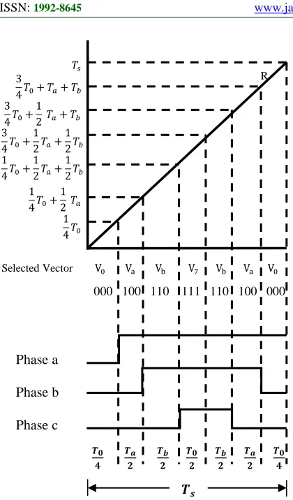
Generates “VS” (Vector Select) signal which indicates the vector that should be present at the output in the correct instant by comparing the ramp signal “R” with different time instants to produce the “symmetric sequence” modulation technique as shown in figure 11, the neural network which implements this function is shown in figure 12
Sec
𝑽𝒂
𝑽𝒃
𝐍𝟏𝟏
𝐍𝟐𝟏
𝐍𝟑𝟏
𝐍𝟒𝟏
𝐍𝟔𝟏
[image:6.612.106.270.323.689.2]Figure 11: Generation of VS Command during Complete Sampling Period in Sector 1
Figure 12: ANN for Producing the VS Command
3.5.1.1 1st hidden layer:
This layer triggers the change of the output vector Each neuron in the first layer (Nx1) will fire when “R” increases above the horizontal lines, which
represents points in time at which the output vector should be changed.
The weight, input and output matrices for the 1st hidden layer are defined as follows:
W1=
⎣ ⎢ ⎢ ⎢ ⎢
⎡11 −0.25−0.25 −0.50 00
1 −0.25 −0.5 −0.5
1 −0.75 −0.5 −0.5
1 −0.75 −0.5 −1
1 −0.75 −1 −1 ⎦⎥
⎥ ⎥ ⎥ ⎤
P1=�
R T0
Ta
Tb
�
O1=
⎣ ⎢ ⎢ ⎢ ⎢ ⎢
⎡ hardlim(Rhardlim(R−0.25T−0.25T0)
0−0.5Ta)
hardlim(R−0.25T0−0.5Ta−0.5Tb)
hardlim(R−0.75T0−0.5Ta−0.5Tb)
hardlim(R−0.75T0−0.5Ta−Tb)
hardlim(R−0.75T0−Ta−Tb) ⎦
⎥ ⎥ ⎥ ⎥ ⎥ ⎤
For example, N11, will fire when R≥0.25T0 ,
N21, will fire when R≥0.25T0+ 0.5Ta and so on.
All results are summarized in table 6.
Table 6: Firing Conditions for Neurons of the 1st
Hidden Layer for the “Vector Selector” ANN
Nx1 Ox1= 1 if
N11 R≥0.25T0
N21 R≥0.25T
0+ 0.5Ta
N31 R≥0.25T
0+ 0.5Ta+ 0.5Tb
N41 R≥0.75T
0+ 0.5Ta+ 0.5Tb
N51 R≥0.75T
0+ 0.5Ta+ Tb
N61 R≥0.75T
0+ Ta+ Tb
3.5.1.2 2nd hidden layer
This layer produces a code that represents the correct “VS” command.
The weight, input and output matrices for the 2nd hidden layer are defined as follows:
W2=�
−2 0 0 0 0 1 1
1 −1 0 0 1 −1 −1
0 1 −1 1 −1 0 −1
0 0 1 −1 0 0 −1
�
R 34𝑇0+𝑇𝑎+𝑇𝑏
3
4𝑇0+12 𝑇𝑎+𝑇𝑏 3
4𝑇0+12𝑇𝑎+12𝑇𝑏 1
4𝑇0+12𝑇𝑎+12𝑇𝑏 14𝑇0+12 𝑇𝑎
14𝑇0
𝑇𝑠
Selected Vector V0 Va Vb V7 Vb Va V0
000 100 110 111 110 100 000
𝑻𝟎
𝟒 𝑻𝒂
𝟐 𝑻𝒃
𝟐 𝑻𝟎
𝟐 𝑻𝒃
𝟐 𝑻𝒂
𝟐 𝑻𝟎
𝟒
Phase a
Phase b
Phase c
𝑻𝒔
R
T0
Ta
Tb
1
VS
𝐍𝟏𝟏
𝐍𝟐𝟏
𝐍𝟑𝟏
𝐍𝟒𝟏
𝐍𝟔𝟏
𝐍𝟓𝟏
𝐍𝟏𝟐
𝐍𝟐𝟐
𝐍𝟑𝟐
[image:7.612.96.293.477.660.2]P2=
⎣ ⎢ ⎢ ⎢ ⎢ ⎢ ⎢ ⎡O11
O12
O13
O14
O15
O16
1⎦⎥ ⎥ ⎥ ⎥ ⎥ ⎥ ⎤
O2=
⎣ ⎢ ⎢ ⎢
⎡ hardlim(−2O11+ O61+ 1)
hardlim(O11−O21+ O51−O16−1)
hardlim(O12−O31+ O14−O51−1)
hardlim(O31−O14−1) ⎦
⎥ ⎥ ⎥ ⎤
N12, will fire (indicating that V0 should be present at
the output) when,
−2O11+ O61+ 1≥0
This is possible when
• O11= 0 AND O16= 0, i.e., R < 0.25T0 AND
R < 0.75T0+ Ta+ Tb (interval 1 in figure 11)
OR
• O11= 1 AND O
6
1 = 1, i.e., R > 0.25T
0 AND
R > 0.75T0+ Ta+ Tb (interval 7 in figure 11)
N12, will also fire if O11= 0 AND O16= 1 but this
case is not applicable because this means that
R < 0.25T0AND R > 0.75T0+ Ta+ Tb which is
not possible.
[image:8.612.325.522.208.315.2]Possible input combinations and the corresponding outputs for N12 are summarized in table 7.
Table 7: Input Combinations of 𝑁12 for the “Vector
Selector” ANN
O11 O61 O12 Interval
0 0 1 1
0 1 1 N/A
1 0 0 N/A
1 1 1 7
Similarly, N22 will fire (indicating that 𝑉𝑎 should be present at the output) when,
O11−O12+ O15−O61−1≥0
N32, will fire (indicating that Vb should be present at
the output) when,
O12−O31+ O14−O15−1≥0
N42, will fire (indicating that V7 should be present at
the output) when,
O13−O41−1≥0
3.5.1.3 Outputlayer:
This layer implements a bit-wise NOT function on the output of the 2nd hidden layer to produce the “VS” vector
Where, VS = [VS1 VS2 VS3 VS4]t
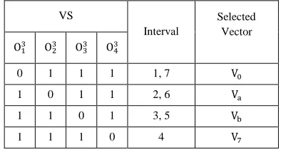
[image:8.612.142.261.525.615.2]The output of the “Vector Selector” ANN for Two-Level SVM is summarized in table 8
Table 8: Output of the “Vector Selector” ANN
VS
Interval
Selected Vector O13 O23 O33 O43
0 1 1 1 1, 7 V0
1 0 1 1 2, 6 Va
1 1 0 1 3, 5 Vb
1 1 1 0 4 V7
3.5.2 Vector decoder
Ensures that the appropriate vector is present at the output in the correct instant so that the inverter switches are switched ON or OFF according to the selected modulation scheme.
The output vector Vout can assume one of four values (Va,Vb,V0 orV7) at different instants in the sampling period Ts
The neural network used to implement this function is shown in figure 13.
3.5.2.1 1st Hidden layer:
The purpose of this layer is to select one of the 4 vectors (V0, Va, Vband V7) and pass it to the next layer. The selected vector depends on the value of the “VS” vector.
This layer contains 12 neurons divided into 4 groups of 3 neurons each (3 neurons for each one of the 4 input vectors), each neuron in this layer represents a ANN switch port, where the 3 neurons of each group is enabled/disabled by a 0/1from the respective bit in the “VS” vector, as shown in table 8
3.5.2.2 2nd Hidden layer
This layer contains 3 neurons, the input to each neuron is similar elements in the 4 vectors so that each neuron passes one element of the selected vector to the output layer. The output of this layer represents the states of the 3 upper inverter switches.
P2=
⎣ ⎢ ⎢ ⎢ ⎢ ⎢ ⎢ ⎢ ⎢ ⎢ ⎢ ⎢ ⎢ ⎡O11
O12
O13
O14
O15
O16
O17
O18
O19
O101
O111
O121 ⎦
⎥ ⎥ ⎥ ⎥ ⎥ ⎥ ⎥ ⎥ ⎥ ⎥ ⎥ ⎥ ⎤
=
⎣ ⎢ ⎢ ⎢ ⎢ ⎢ ⎢ ⎢ ⎢ ⎢ ⎢ ⎢ ⎡VV01
02
V03
Va1
Va2
Va3
Vb1
Vb2
Vb3
V71
V72
V73⎦
⎥ ⎥ ⎥ ⎥ ⎥ ⎥ ⎥ ⎥ ⎥ ⎥ ⎥ ⎤
W2=�
1 0 0 1 0 0 1 0 0 1 0 0 0 1 0 0 1 0 0 1 0 0 1 0
0 0 1 0 0 1 0 0 1 0 0 1�
O2=�purelin(Vpurelin(V01+ Va1+ Vb1+ V71) 02+ Va2+ Vb2+ V72)
purelin(V03+ Va3+ Vb3+ V73)
�
3.5.2.3 Output layer:
[image:9.612.89.523.197.637.2]This layer implements the NOT function on the output from the 2nd hidden layer to produce the states of the lower 3 inverter switches.
Figure 13: “Vector Decoder” ANN
4. SIMULATION RESULTS
The two-level ANN SVM generator is employed inside a scalar control drive system to validate its operation. Figure 14 shows the block diagram of
the closed loop V/Hz scalar control used in the simulation.
The angular velocity, is compared with the reference speed, 𝜔𝑀∗ The speed error signal, ∆𝜔𝑀, is applied to a slip controller, usually of the PI type, which generates the reference slip speed, 𝜔𝑆𝐿∗ . The slip speed must be limited for stability and over-current prevention. The reference synchronous speed 𝜔𝑆𝑦𝑛∗ is obtained by adding 𝜔𝑆𝐿∗ to 𝜔𝑀 .The latter signal used to generate the reference values,
𝑉∗and 𝜔∗ [5].
Figure 14: Closed Loop V/Hz Scalar Control
Figure 15: Rotor Speed 𝜔𝑀
𝑽𝟎
𝑽𝐚
𝑽𝐛
𝑽𝟕
VS
𝒔𝟏
𝒔𝟐
𝒔𝟑
𝒔𝟒
𝒔𝟓
𝒔𝟔
3* ANN
Switch Ports
3* ANN
Switch Ports
3* ANN
Switch Ports
3* ANN
Switch Ports
ωM∗
SVM Generator
Inverter
ωM
∆ωM P-I ωSL∗
+ Limiter
𝜔𝑆𝑦𝑛∗
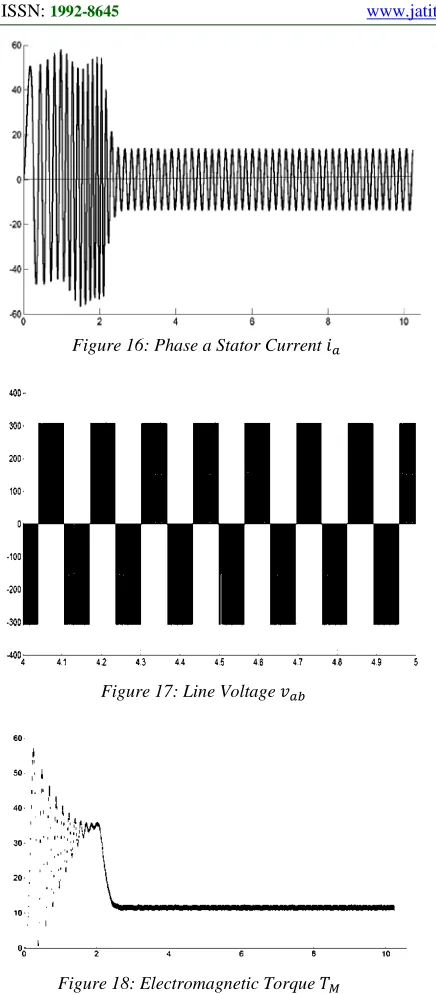
[image:9.612.320.522.236.383.2]Figure 16: Phase a Stator Current 𝑖𝑎
Figure 17: Line Voltage 𝑣𝑎𝑏
Figure 18: Electromagnetic Torque 𝑇𝑀
5. CONCLUSION
Space vector pulse width modulation (SVPWM) can be implemented using a set of interconnected artificial neural networks, where each network achieves a certain step in the SVPWM algorithm. The proposed SVPWM scheme was employed inside a closed loop v/Hz scalar control system and simulated using MATLAB Simulink to verify its operation.
REFERENCES:
[1] Muhammad H. Rashid, “Power Electronics Hand Book”, Academic Press, Academic Press Series in Engineering, First Edition, 2001, ISBN-0125816502
[2] Bimal K. Bose, “Modern Power electronic and AC Drives”, Prentice Hall, First Edition, 2001, ISBN-0130167436
[3] Subrata K. Mondal, João O. P. Pinto and Bimal K. Bose, “A Neural-Network-Based Space-Vector PWM Controller for a Three-Level Voltage-Fed Inverter Induction Motor Drive”, IEEE transactions on Industry Applications, VOL. 38, No. 3, May/June 2002
[4] Prasad, V. H., Master of Science In Electrical Engineering, “Analysis and Comparison of Space Vector Modulation schemes for Three-Leg and Four-Three-Leg Voltage Source inverters”, Virginia Polytechnic Institute and State University, 1997