WRL 89 7 pdf

WRL

Research Report 89/7

Available

Instruction-Level Parallelism for

Superscalar and

Superpipelined Machines

research relevant to the design and application of high performance scientific computers. We test our ideas by designing, building, and using real systems. The systems we build are research prototypes; they are not intended to become products.

There is a second research laboratory located in Palo Alto, the Systems Research Cen-ter (SRC). Other Digital research groups are located in Paris (PRL) and in Cambridge, Massachusetts (CRL).

Our research is directed towards mainstream high-performance computer systems. Our prototypes are intended to foreshadow the future computing environments used by many Digital customers. The long-term goal of WRL is to aid and accelerate the development of high-performance uni- and multi-processors. The research projects within WRL will address various aspects of high-performance computing.

We believe that significant advances in computer systems do not come from any single technological advance. Technologies, both hardware and software, do not all advance at the same pace. System design is the art of composing systems which use each level of technology in an appropriate balance. A major advance in overall system performance will require reexamination of all aspects of the system.

We do work in the design, fabrication and packaging of hardware; language processing and scaling issues in system software design; and the exploration of new applications areas that are opening up with the advent of higher performance systems. Researchers at WRL cooperate closely and move freely among the various levels of system design. This allows us to explore a wide range of tradeoffs to meet system goals.

We publish the results of our work in a variety of journals, conferences, research reports, and technical notes. This document is a research report. Research reports are normally accounts of completed research and may include material from earlier technical notes. We use technical notes for rapid distribution of technical material; usually this represents research in progress.

Research reports and technical notes may be ordered from us. You may mail your order to:

Technical Report Distribution

DEC Western Research Laboratory, UCO-4 100 Hamilton Avenue

Palo Alto, California 94301 USA

Reports and notes may also be ordered by electronic mail. Use one of the following addresses:

Digital E-net: DECWRL::WRL-TECHREPORTS DARPA Internet: [email protected] CSnet: [email protected] UUCP: decwrl!wrl-techreports

Superscalar and Superpipelined Machines

Norman P. Jouppi and David W. Wall

Superscalar machines can issue several instructions per cycle. Super-pipelined machines can issue only one instruction per cycle, but they have cycle times shorter than the latency of any functional unit. In this paper these two techniques are shown to be roughly equivalent ways of exploiting instruction-level parallelism. A parameterizable code reorganization and simulation system was developed and used to measure instruction-level parallelism for a series of benchmarks. Results of these simulations in the presence of various compiler optimizations are presented. The average

de-gree of superpipelining metric is introduced. Our simulations suggest that

this metric is already high for many machines. These machines already ex-ploit all of the instruction-level parallelism available in many non-numeric applications, even without parallel instruction issue or higher degrees of pipelining.

This is a preprint of a paper that will be presented at the 3rd International Conference on Architectural Support for

Programming Languages and Operating Systems, IEEE and ACM, Boston, Massachusetts, April 3-6, 1989. An early draft of this paper appeared as WRL Technical Note TN-2.

puter performance since the first computer was designed. The most significant advances in uniprocessor performance have come from exploiting advances in implementation technology. Architectural innovations have also played a part, and one of the most significant of these over the last decade has been the rediscovery of RISC architectures. Now that RISC architectures have gained acceptance both in scientific and marketing circles, computer architects have been thinking of new ways to improve uniprocessor performance. Many of these proposals such as VLIW [12], superscalar, and even relatively old ideas such as vector processing try to improve computer performance by exploiting instruction-level parallelism. They take advantage of this parallelism by issuing more than one instruction per cycle explicitly (as in VLIW or superscalar machines) or implicitly (as in vector machines). In this paper we will limit ourselves to improv-ing uniprocessor performance, and will not discuss methods of improvimprov-ing application perfor-mance by using multiple processors in parallel.

As an example of instruction-level parallelism, consider the two code fragments in Figure 1. The three instructions in (a) are independent; there are no data dependencies between them, and in theory they could all be executed in parallel. In contrast, the three instructions in (b) cannot be executed in parallel, because the second instruction uses the result of the first, and the third instruction uses the result of the second.

Load C1<-23(R2) Add R3<-R3+1 Add R3<-R3+1 Add R4<-R3+R2 FPAdd C4<-C4+C3 Store 0[R4]<-R0

(a) parallelism=3 (b) parallelism=1

Figure 1: Instruction-level parallelism

In Section 2 we present a machine taxonomy helpful for understanding the duality of opera-tion latency and parallel instrucopera-tion issue. Secopera-tion 3 describes the compilaopera-tion and simulaopera-tion environment we used to measure the parallelism in benchmarks and its exploitation by different architectures. Section 4 presents the results of these simulations. These results confirm the duality of superscalar and superpipelined machines, and show serious limits on the instruction-level parallelism available in most applications. They also show that most classical code op-timizations do nothing to relieve these limits. The importance of cache miss latencies, design complexity, and technology constraints are considered in Section 5. Section 6 summarizes the results of the paper.

2. A Machine Taxonomy

There are several different ways to execute instructions in parallel. Before we examine these methods in detail, we need to start with some definitions:

operation latency The time (in cycles) until the result of an instruction is available for use as an operand in a subsequent instruction. For example, if the result of an Add instruction can be used as an operand of an instruction that is issued in the cycle after the Add is issued, we say that the Add has an operation latency of one.

simple operations The vast majority of operations executed by the machine. Operations such as integer add, logical ops, loads, stores, branches, and even floating-point addition and multiplication are simple operations. Not included as simple operations are instructions which take an order of magnitude more time and occur less frequently, such as divide and cache misses.

instruction class A group of instructions all issued to the same type of functional unit.

issue latency The time (in cycles) required between issuing two instructions. This can vary depending on the instruction classes of the two instructions.

2.1. The Base Machine

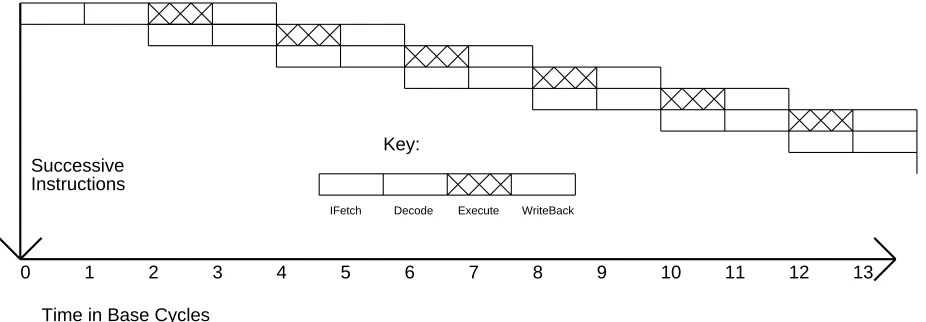
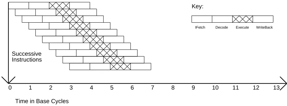
In order to properly compare increases in performance due to exploitation of instruction-level parallelism, we define a base machine that has an execution pipestage parallelism of exactly one. This base machine is defined as follows:

•Instructions issued per cycle = 1

•Simple operation latency measured in cycles = 1

•Instruction-level parallelism required to fully utilize = 1

Time in Base Cycles

0 1 2 3 4 5 6 7 8 9 10 11 12 13

Successive Instructions

IFetch Decode WriteBack

Key:

Execute

Figure 2: Execution in a base machine

2.2. Underpipelined Machines

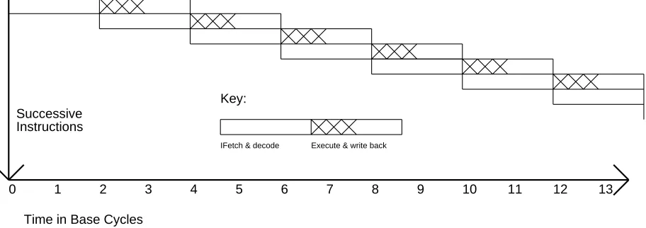
The single-cycle latency of simple operations also sets the base machine cycle time. Although one could build a base machine where the cycle time was much larger than the time required for each simple operation, it would be a waste of execution time and resources. This would be an underpipelined machine. An underpipelined machine that executes an operation and writes back the result in the same pipestage is shown in Figure 3.

13 12 11 10 9

8 7 6 5 4 3 2 1 0

Time in Base Cycles Successive

Instructions

Execute & write back

Key:

IFetch & decode

Figure 3: Underpipelined: cycle > operation latency

to write back the result has been pipelined into the next pipestage. Then the base cycle time is simply the minimum time required to do a fixed-point add and bypass the result to the next instruction. In this sense machines like the Stanford MIPS chip [8] are underpipelined, because they read operands out of the register file, do an ALU operation, and write back the result all in one cycle.

Another example of underpipelining would be a machine like the Berkeley RISC II chip [10], where loads can only be issued every other cycle. Obviously this reduces the instruction-level parallelism below one instruction per cycle. An underpipelined machine that can only issue an instruction every other cycle is illustrated in Figure 4. Note that this machine’s performance is the same as the machine in Figure 3, which is half of the performance attainable by the base machine. Successive Instructions 13 12 11 10 9 8 7 6 5 4 3 2 1 0

Time in Base Cycles

Execute WriteBack Decode

IFetch

Key:

Figure 4: Underpipelined: issues < 1 instr. per cycle

In summary, an underpipelined machine has worse performance than the base machine be-cause it either has:

•a cycle time greater than the latency of a simple operation, or

•it issues less than one instruction per cycle.

For this reason underpipelined machines will not be considered in the rest of this paper.

2.3. Superscalar Machines

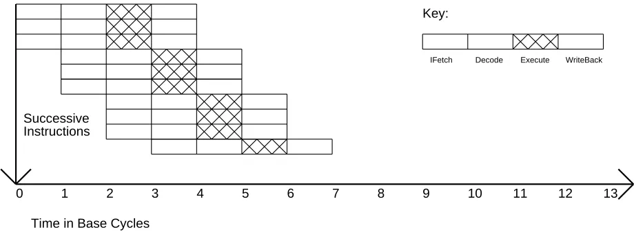
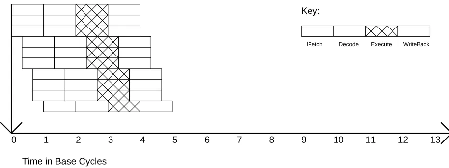
As their name suggests, superscalar machines were originally developed as an alternative to vector machines. A superscalar machine of degree n can issue n instructions per cycle. A super-scalar machine could issue all three parallel instructions in Figure 1(a) in the same cycle. Super-scalar execution of instructions is illustrated in Figure 5.

13 12 11 10 9 8 7 6 5 4 3 2 1 0

Time in Base Cycles Successive Instructions Execute Key: WriteBack Decode IFetch

Figure 5: Execution in a superscalar machine (n=3)

Formalizing a superscalar machine according to our definitions:

•Instructions issued per cycle = n

•Simple operation latency measured in cycles = 1

•Instruction-level parallelism required to fully utilize = n

A superscalar machine can attain the same performance as a machine with vector hardware. Consider the operations performed when a vector machine executes a vector load chained into a vector add, with one element loaded and added per cycle. The vector machine performs four operations: load, floating-point add, a fixed-point add to generate the next load address, and a compare and branch to see if we have loaded and added the last vector element. A superscalar machine that can issue a fixed-point, floating-point, load, and a branch all in one cycle achieves the same effective parallelism.

2.3.1. VLIW Machines

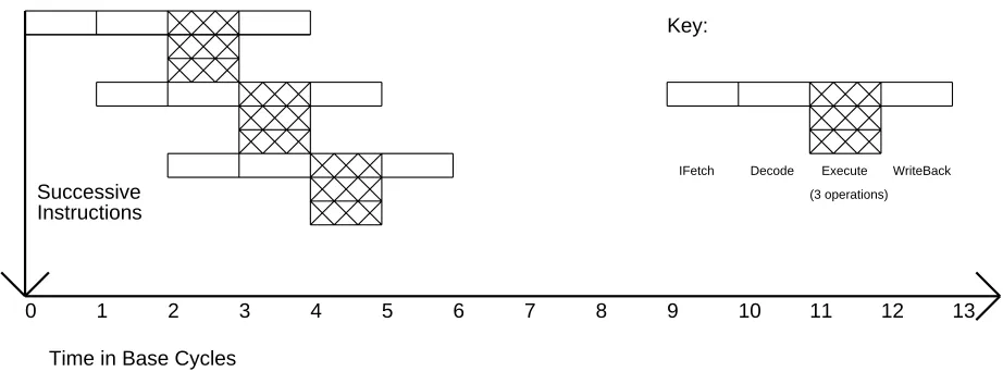
VLIW, or very long instruction word, machines typically have instructions hundreds of bits long. Each instruction can specify many operations, so each instruction exploits instruction-level parallelism. Many performance studies have been performed on VLIW machines [12]. The ex-ecution of instructions by an ideal VLIW machine is shown in Figure 6. Each instruction specifies multiple operations, and this is denoted in the Figure by having multiple crosshatched execution stages in parallel for each instruction.

VLIW machines are much like superscalar machines, with three differences.

Successive Instructions

Time in Base Cycles

0 1 2 3 4 5 6 7 8 9 10 11 12 13

Key:

Decode Execute WriteBack IFetch

(3 operations)

Figure 6: Execution in a VLIW machine

in a given cycle is performed at compile time in a VLIW machine, and at run time in a super-scalar machine. Thus the instruction decode logic for the VLIW machine should be much simpler than the superscalar.

A second difference is that when the available instruction-level parallelism is less than that exploitable by the VLIW machine, the code density of the superscalar machine will be better. This is because the fixed VLIW format includes bits for unused operations while the superscalar machine only has instruction bits for useful operations.

A third difference is that a superscalar machine could be object-code compatible with a large family of non-parallel machines, but VLIW machines exploiting different amounts of parallelism would require different instruction sets. This is because the VLIW’s that are able to exploit more parallelism would require larger instructions.

In spite of these differences, in terms of run time exploitation of instruction-level parallelism, the superscalar and VLIW will have similar characteristics. Because of the close relationship between these two machines, we will only discuss superscalar machines in general and not dwell further on distinctions between VLIW and superscalar machines.

2.3.2. Class Conflicts

There are two ways to develop a superscalar machine of degree n from a base machine. 1. Duplicate all functional units n times, including register ports, bypasses, busses,

and instruction decode logic.

2. Duplicate only the register ports, bypasses, busses, and instruction decode logic.

machine. (We will not consider superscalar machines or any other machines that issue instruc-tions out of order. Techniques to reorder instrucinstruc-tions at compile time instead of at run time are almost as good [6, 7, 17], and are dramatically simpler than doing it in hardware.)

2.4. Superpipelined Machines

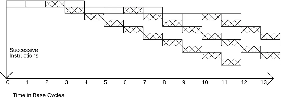
Superpipelined machines exploit instruction-level parallelism in another way. In a super-pipelined machine of degree m, the cycle time is 1/m the cycle time of the base machine. Since a fixed-point add took a whole cycle in the base machine, given the same implementation tech-nology it must take m cycles in the superpipelined machine. The three parallel instructions in Figure 1(a) would be issued in three successive cycles, and by the time the third has been issued, there are three operations in progress at the same time. Figure 7 shows the execution of instruc-tions by a superpipelined machine.

Formalizing a superpipelined machine according to our definitions:

•Instructions issued per cycle = 1, but the cycle time is 1/m of the base machine

•Simple operation latency measured in cycles = m

•Instruction-level parallelism required to fully utilize = m

13 12 11 10 9

8 7 6 5 4 3 2 1 0

Time in Base Cycles Successive

Instructions

Execute

Key:

WriteBack Decode

IFetch

Figure 7: Superpipelined execution (m=3)

2.5. Superpipelined Superscalar Machines

Since the number of instructions issued per cycle and the cycle time are theoretically or-thogonal, we could have a superpipelined superscalar machine. A superpipelined superscalar machine of degree (m,n) has a cycle time 1/m that of the base machine, and it can execute n instructions every cycle. This is illustrated in Figure 8.

IFetch Decode WriteBack

Key:

Execute

Time in Base Cycles

0 1 2 3 4 5 6 7 8 9 10 11 12 13

Figure 8: A superpipelined superscalar (n=3,m=3)

Formalizing a superpipelined superscalar machine according to our definitions:

•Instructions issued per cycle = n, and the cycle time is 1/m that of the base machine

•Simple operation latency measured in cycles = m

•Instruction-level parallelism required to fully utilize = n*m

2.6. Vector Machines

Although vector machines also take advantage of (unrolled-loop) instruction-level parallelism, whether a machine supports vectors is really independent of whether it is a superpipelined, su-perscalar, or base machine. Each of these machines could have an attached vector unit. However, to the extent that the highly parallel code was run in vector mode, it would reduce the use of superpipelined or superscalar aspects of the machine to the code that had only moderate instruction-level parallelism. Figure 9 shows serial issue (for diagram readability only) and parallel execution of vector instructions. Each vector instruction results in a string of operations, one for each element in the vector.

2.7. Supersymmetry

The most important thing to keep in mind when comparing superscalar and superpipelined machines of equal degree is that they have basically the same performance.

13 12 11 10 9

8 7 6 5 4 3 2 1 0

Time in Base Cycles Successive

Instructions

Figure 9: Execution in a vector machine

three instructions in successive cycles. Each of these machines issues instructions at the same rate, so superscalar and superpipelined machines of equal degree have basically the same perfor-mance.

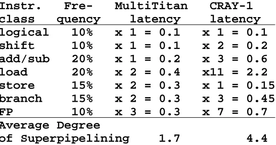
So far our assumption has been that the latency of all operations, or at least the simple opera-tions, is one base machine cycle. As we discussed previously, no known machines have this characteristic. For example, few machines have one cycle loads without a possible data interlock either before or after the load. Similarly, few machines can execute floating-point operations in one cycle. What are the effects of longer latencies? Consider the MultiTitan [9], where ALU operations are one cycle, but loads, stores, and branches are two cycles, and all floating-point operations are three cycles. The MultiTitan is therefore a slightly superpipelined machine. If we multiply the latency of each instruction class by the frequency we observe for that instruction class when we perform our benchmark set, we get the average degree of superpipelining. The average degree of superpipelining is computed in Table 1 for the MultiTitan and the CRAY-1. To the extent that some operation latencies are greater than one base machine cycle, the remain-ing amount of exploitable instruction-level parallelism will be reduced. In this example, if the average degree of instruction-level parallelism in slightly parallel code is around two, the Mul-tiTitan should not stall often because of data-dependency interlocks, but data-dependency inter-locks should occur frequently on the CRAY-1.

3. Machine Evaluation Environment

Instr. Fre- MultiTitan CRAY-1 class quency latency latency logical 10% x 1 = 0.1 x 1 = 0.1 shift 10% x 1 = 0.1 x 2 = 0.2 add/sub 20% x 1 = 0.2 x 3 = 0.6 load 20% x 2 = 0.4 x11 = 2.2 store 15% x 2 = 0.3 x 1 = 0.15 branch 15% x 2 = 0.3 x 3 = 0.45 FP 10% x 3 = 0.3 x 7 = 0.7 Average Degree

of Superpipelining 1.7 4.4

Table 1: Average degree of superpipelining

To specify the pipeline structure and functional units, we need to be able to talk about specific instructions. We therefore group the MultiTitan operations into fourteen classes, selected so that operations in a given class are likely to have identical pipeline behavior in any machine. For example, integer add and subtract form one class, integer multiply forms another class, and single-word load forms a third class.

For each of these classes we can specify an operation latency. If an instruction requires the result of a previous instruction, the machine will stall unless the operation latency of the previous instruction has elapsed. The compile-time pipeline instruction scheduler knows this and schedules the instructions in a basic block so that the resulting stall time will be minimized.

We can also group the operations into functional units, and specify an issue latency and mul-tiplicity for each. For instance, suppose we want to issue an instruction associated with a func-tional unit with issue latency 3 and multiplicity 2. This means that there are two units we might use to issue the instruction. If both are busy then the machine will stall until one is idle. It then issues the instruction on the idle unit, and that unit is unable to issue another instruction until three cycles later. The issue latency is independent of the operation latency; the former affects later operations using the same functional unit, and the latter affects later instructions using the result of this one. In either case, the pipeline instruction scheduler tries to minimize the resulting stall time.

Superscalar machines may have an upper limit on the number of instructions that may be issued in the same cycle, independent of the availability of functional units. We can specify this upper limit. If no upper limit is desired, we can set it to the total number of functional units.

4. Results

We used our programmable reorganization and simulation system to investigate the perfor-mance of various superpipelined and superscalar machine organizations. We ran eight different benchmarks on each different configuration. All of the benchmarks are written in Modula-2 except for yacc.

ccom Our own C compiler.

grr A PC board router.

linpack Linpack, double precision, unrolled 4x unless noted otherwise.

livermore The first 14 Livermore Loops, double precision, not unrolled unless noted otherwise.

met Metronome, a board-level timing verifier.

stan The collection of Hennessy benchmarks from Stanford (including puzzle, tower, queens, etc.).

whet Whetsones.

yacc The Unix parser generator.

Unless noted otherwise, the effects of cache misses and systems effects such as interrupts and TLB misses are ignored in the simulations. Moreover, when available instruction-level paral-lelism is discussed, it is assumed that all operations execute in one cycle. To determine the actual number of instructions issuable per cycle in a specific machine, the available parallelism must be divided by the average operation latency.

4.1. The Duality of Latency and Parallel Issue

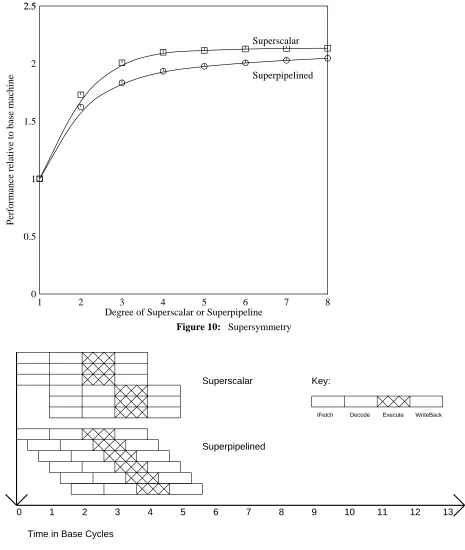
In section 2.7 we stated that a superpipelined machine and an ideal superscalar machine (i.e., without class conflicts) should have the same performance, since they both have the same num-ber of instructions executing in parallel. To confirm this we simulated the eight benchmarks on an ideal base machine, and on superpipelined and ideal superscalar machines of degrees 2 through 8. Figure 10 shows the results of this simulation. The superpipelined machine actually has less performance than the superscalar machine, but the performance difference decreases with increasing degree.

Consider a superscalar and superpipelined machine, both of degree three, issuing a basic block of six independent instructions (see Figure 11). The superscalar machine will issue the last in-struction at time t (assuming execution starts at t ). In contrast, the superpipelined machine will_{1 0} take 1/3 cycle to issue each instruction, so it will not issue the last instruction until time t_5/3. Thus although the superscalar and superpipelined machines have the same number of instruc-tions executing at the same time in the steady state, the superpipelined machine has a larger startup transient and it gets behind the superscalar machine at the start of the program and at each branch target. This effect diminishes as the degree of the superpipelined machine increases and all of the issuable instructions are issued closer and closer together. This effect is seen in Figure 10 as the superpipelined performance approaches that of the ideal superscalar machine with in-creasing degree.

1 2 3 4 5 6 7 8 Degree of Superscalar or Superpipeline

0 2.5

0.5 1 1.5 2 2.5

Performance relative to base machine

Superpipelined Superscalar

Figure 10: Supersymmetry

Execute

Key:

WriteBack Decode

IFetch

Time in Base Cycles

0 1 2 3 4 5 6 7 8 9 10 11 12 13

Superscalar

Superpipelined

Figure 11: Start-up in superscalar vs. superpipelined

super-pipelined cycle. Then in a superscalar machine of degree 3 the latency of a logical or move operation might be 2/3 longer than in a superpipelined machine of degree 3. Since the latency is longer for the superscalar machine, the superpipelined machine will perform better than a super-scalar machine of equal degree. In general, when the inherent operation latency is divided by the clock period, the remainder is less on average for machines with shorter clock periods. We have not quantified the effect of this difference to date.

4.2. Limits to Instruction-Level Parallelism

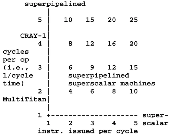
Studies dating from the late 1960’s and early 1970’s [14, 15] and continuing today have ob-served average instruction-level parallelism of around 2 for code without loop unrolling. Thus, for these codes there is not much benefit gained from building a machine with superpipelining greater than degree 3 or a superscalar machine of degree greater than 3. The instruction-level parallelism required to fully utilize machines is plotted in Figure 12. On this graph, the X dimen-sion is the degree of superscalar machine, and the Y dimendimen-sion is the degree of superpipelining. Since a superpipelined superscalar machine of only degree (2,2) would require an instruction-level parallelism of 4, it seems unlikely that it would ever be worth building a superpipelined superscalar machine for moderately or slightly parallel code. The superpipelining axis is marked with the average degree of superpipelining in the CRAY-1 that was computed in Section 2.7. From this it is clear that vast amounts of instruction-level parallelism would be required before the issuing of multiple instructions per cycle would be warranted in the CRAY-1.

superpipelined |

5 | 10 15 20 25 |

CRAY-1|

4 | 8 12 16 20 cycles |

per op |

(i.e., 3 | 6 9 12 15 1/cycle | superpipelined

time) | superscalar machines 2 | 4 6 8 10 MultiTitan|

|

1 +--- super-1 2 3 4 5 scalar instr. issued per cycle

Figure 12: Parallelism required for full utilization

is-sue. We simulated the performance of the CRAY-1 assuming single cycle functional unit latency and actual functional unit latencies, and the results are given in Figure 13.

1 2 3 4 5 6 7 8

Instruction issue multiplicity 0

120

20 40 60 80 100

Performance (MIPS)

all latencies = 1

actual CRAY-1 latencies

Figure 13: Parallel issue with unit and real latencies

As expected, since the CRAY-1 already executes several instructions concurrently due to its average degree of superpipelining of 4.4, there is almost no benefit from issuing multiple instruc-tions per cycle when the actual functional unit latencies are taken into account.

4.3. Variations in Instruction-Level Parallelism

1 2 3 4 5 6 7 8 Instruction issue multiplicity

1 4

2 3

Superscalar performance realtive to base machine

ccom grr

linpack.unroll4x

livermore

metronome stanford

whetsones

yacc

Figure 14: Instruction-level parallelism by benchmark

4.4. Effects of Optimizing Compilers

Compilers have been useful in detecting and exploiting instruction-level parallelism. Highly parallel loops can be vectorized [3]. Somewhat less parallel loops can be unrolled and then trace-scheduled [5] or software-pipelined [4, 11]. Even code that is only slightly parallel can be scheduled [6, 7, 17] to exploit a superscalar or superpipelined machine.

The effect of loop-unrolling on instruction-level parallelism is shown in Figure 15. The Lin-pack and Livermore benchmarks were simulated without loop unrolling and also unrolled two, four, and ten times. In either case we did the unrolling in two ways: naively and carefully. Naive unrolling consists simply of duplicating the loop body inside the loop, and allowing the normal code optimizer and scheduler to remove redundant computations and to re-order the in-structions to maximize parallelism. Careful unrolling goes farther. In careful unrolling, we reas-sociate long strings of additions or multiplications to maximize the parallelism, and we analyze the stores in the unrolled loop so that stores from early copies of the loop do not interfere with loads in later copies. Both the naive and the careful unrolling were done by hand.

unroll-1 2 4 6 8 10 Number of iterations unrolled

0 7

0.5 1 1.5 2 2.5 3 3.5 4 4.5 5 5.5 6 6.5

Instruction-level parallelism

livermore.naive linpack.naive livermore.careful linpack.careful

Figure 15: Parallelism vs. loop unrolling

ing. One reason for this is that we have only forty temporary registers available, which limits the amount of parallelism we can exploit.

In practice, the peak parallelism was quite high. The parallelism was 11 for the carefully unrolled inner loop of Linpack, and 22 for one of the carefully unrolled Livermore loops. However, in either case there is still a lot of inherently sequential computation, even in important places. Three of the Livermore loops, for example, implement recurrences that benefit little from unrolling. If we spend half the time in a very parallel inner loop, and we manage to make this inner loop take nearly zero time by executing its code in parallel, we only double the speed of the program.

In all cases, cache effects were ignored. If limited instruction caches were present, the actual performance would decline for large degrees of unrolling.

In general, however, classical optimizations can either add to or subtract from parallelism. This is illustrated by the expression graph in Figure 16. If our computation consists of two branches of comparable complexity that can be executed in parallel, then optimizing one branch reduces the parallelism. On the other hand, if the computation contains a bottleneck on which other operations wait, then optimizing the bottleneck increases the parallelism. This argument holds equally well for most global optimizations, which are usually just combinations of local optimizations that require global information to detect. For example, to move invariant code out of a loop, we just remove a large computation and replace it with a reference to a single tem-porary. We also insert a large computation before the loop, but if the loop is executed many times then changing the parallelism of code outside the loop won’t make much difference.

Parallelism = 1.67 Parallelism = 1.33 Parallelism = 1.50

Figure 16: Parallelism vs. compiler optimizations

Global allocation of registers to local and global variables [16] is not usually considered a classical optimization, because it has been widespread only since the advent of machines with large register sets. However, it too can either increase or decrease parallelism. A basic block in which all variables reside in memory must load those variables into registers before it can operate on them. Since these loads can be done in parallel, we would expect to reduce the over-all parover-allelism by globover-ally over-allocating the variables to registers and removing these loads. On the other hand, assignments of new values to these variables may be easier for the pipeline scheduler to re-order if they are assignments to registers rather than stores to memory.

We simulated our test suite with various levels of optimization. Figure 17 shows the results. The leftmost point is the parallelism with no optimization at all. Each time we move to the right, we add a new set of optimizations. In order, these are pipeline scheduling, intra-block optimiza-tions, global optimizaoptimiza-tions, and global register allocation. In this comparison we used 16 registers for expression temporaries and 26 for global register allocation. The dotted and dashed lines allow the different benchmarks to be distinguished, and are not otherwise significant.

0 1 2 3 4 Optimization Level 0 3.5 0.5 1 1.5 2 2.5 3

Base Machine Instruction-Level Parallelism

scheduling scheduling local opt scheduling local opt global opt scheduling local opt global opt reg alloc stan livermore yacc whet ccom met linpack.unroll4x grr

Figure 17: Effect of optimization on parallelism

The behavior of the Livermore benchmark is anomalous. A large decrease in parallelism oc-curs when we add optimization because the inner loops of these benchmarks contain redundant address calculations that are recognized as common subexpressions. For example, without com-mon subexpression elimination the address of A[I] would be computed twice in the expression "A[I] = A[I] + 1". It happens that these redundant calculations are not bottlenecks, so removing them decreases the parallelism.

Global register allocation causes a slight decrease in parallelism for most of the benchmarks. This is because operand loads can be done in parallel, and are removed by register allocation.

The numeric benchmarks Livermore, Linpack, and Whetstones are exceptions to this. Global register allocation increases the parallelism of these three. This is because key inner loops con-tain intermixed references to scalars and to array elements. Loads from the former may appear to depend on previous stores to the latter, because the scheduler must assume that two memory locations are the same unless it can prove otherwise. If global register allocation chooses to keep a scalar in a register instead of memory, this spurious dependency disappears.

the parallelism that is already present. Even the benefit from scheduling varies widely between programs.

5. Other Important Factors

The preceding simulations have concentrated on the duality of latency and parallel instruction issue under ideal circumstances. Unfortunately there are a number of other factors which will have a very important effect on machine performance in reality. In this section we will briefly discuss some of these factors.

5.1. Cache Performance

Cache performance is becoming increasingly important, and it can have a dramatic effect on speedups obtained from parallel instruction execution. Figure 2 lists some cache miss times and the effect of a miss on machine performance. Over the last decade, cycle time has been decreas-ing much faster than main memory access time. The average number of machine cycles per instruction has also been decreasing dramatically, especially when the transition from CISC machines to RISC machines is included. These two effects are multiplicative and result in tremendous increases in miss cost. For example, a cache miss on a VAX 11/780 only costs 60% of the average instruction execution. Thus even if every instruction had a cache miss, the machine performance would only slow down by 60%! However, if a RISC machine like the WRL Titan [13] has a miss, the cost is almost ten instruction times. Moreover, these trends seem to be continuing, especially the increasing ratio of memory access time to machine cycle time. In the future a cache miss on a superscalar machine executing two instructions per cycle could cost well over 100 instruction times!

Machine cycles cycle mem miss miss per time time cost cost instr (ns) (ns) cycles instr VAX11/780 10.0 200 1200 6 .6 WRL Titan 1.4 45 540 12 8.6 ? 0.5 5 350 70 140.0

Table 2: The cost of cache misses

Cache miss effects decrease the benefit of parallel instruction issue. Consider a 2.0cpi (i.e., 2.0 cycles per instruction) machine, where 1.0cpi is from issuing one instruction per cycle, and 1.0 cpi is cache miss burden. Now assume the machine is given the capability to issue three instructions per cycle, to get a net decrease down to 0.5cpi for issuing instructions when data dependencies are taken into account. Performance is proportional to the inverse of the cpi change. Thus the overall performance improvement will be from 1/2.0cpi to 1/1.5cpi, or 33%. This is much less than the improvement of 1/1.0cpi to 1/0.5cpi, or 100%, as when cache misses are ignored.

5.2. Design Complexity and Technology Constraints

two ways, both of which are hard to quantify. First, the added complexity can slow down the machine by adding to the critical path, not only in terms of logic stages but in terms of greater distances to be traversed when crossing a more complicated and bigger machine. As we have seen from our analysis of the importance of latency, hiding additional complexity by adding ex-tra pipeline stages will not make it go away. Also, the machine can be slowed down by having a fixed resource (e.g., good circuit designers) spread thinner because of a larger design. Finally, added complexity can negate performance improvements by increasing time to market. If the implementation technologies are fixed at the start of a design, and processor performance is quadrupling every three years, a one or two year slip because of extra complexity can easily negate any additional performance gained from the complexity.

Since a superpipelined machine and a superscalar machine have approximately the same per-formance, the decision as to whether to implement a superscalar or a superpipelined machine should be based largely on their feasibility and cost in various technologies. For example, if a TTL machine was being built from off-the-shelf components, the designers would not have the freedom to insert pipeline stages wherever they desired. For example, they would be required to use several multiplier chips in parallel (i.e., superscalar), instead of pipelining one multiplier chip more heavily (i.e., superpipelined). Another factor is the shorter cycle times required by the superpipelined machine. For example, if short cycle times are possible though the use of fast interchip signalling (e.g., ECL with terminated transmission lines), a superpipelined machine would be feasible. However, relatively slow TTL off-chip signaling might require the use of a superscalar organization. In general, if it is feasible, a superpipelined machine would be preferred since it only pipelines existing logic more heavily by adding latches instead of duplicating functional units as in the superscalar machine.

6. Concluding Comments

In this paper we have shown superscalar and superpipelined machines to be roughly equiv-alent ways to exploit instruction-level parallelism. The duality of latency and parallel instruction issue was documented by simulations. Ignoring class conflicts and implementation complexity, a superscalar machine will have slightly better performance (by less than 10% on our benchmarks) than a superpipelined machine of the same degree due to the larger startup transient of the superpipelined machine. However, class conflicts and the extra complexity of parallel over pipelined instruction decode could easily negate this advantage. These tradeoffs merit in-vestigation in future work.

The available parallelism after normal optimizations and global register allocation ranges from a low of 1.6 for Yacc to 3.2 for Linpack. In heavily parallel programs like the numeric benchmarks, we can improve the parallelism somewhat by loop unrolling. However, dramatic improvements are possible only when we carefully restructure the unrolled loops. This restruc-turing requires us to use knowledge of operator associativity, and to do interprocedural alias analysis to determine when memory references are independent. Even when we do this, the performance improvements are limited by the non-parallel code in the application, and the im-provements in parallelism are not as large as the degree of unrolling. In any case, loop unrolling is of little use in non-parallel applications like Yacc or the C compiler.

on the parallelism available in non-numeric applications, even when it had a large effect on the performance. Optimization had a larger effect on the parallelism of numeric benchmarks, but the size and even the direction of the the effect depended heavily on the code’s context and the availability of temporary registers.

Finally, many machines already exploit most of the parallelism available in non-numeric code because they can issue an instruction every cycle but have operation latencies greater than one. Thus for many applications, significant performance improvements from parallel instruction is-sue or higher degrees of pipelining should not be expected.

7. Acknowledgements

Jeremy Dion, Mary Jo Doherty, John Ousterhout, Richard Swan, Neil Wilhelm, and the reviewers provided valuable comments on an early draft of this paper.

References

[1] Acosta, R. D., Kjelstrup, J., and Torng, H. C.

An Instruction Issuing Approach to Enhancing Performance in Multiple Functional Unit Processors.

IEEE Transactions on Computers C-35(9):815-828, September, 1986.

[2] Aho, Alfred V., Sethi, Ravi, and Ullman, Jeffrey D. Compilers: Principles, Techniques, and Tools. Addison-Wesley, 1986.

[3] Allen, Randy, and Kennedy, Ken.

Automatic Translation of FORTRAN Programs to Vector Form.

ACM Transactions on Programming Languages and Systems 9(4):491-542, October, 1987.

[4] Charlesworth, Alan E.

An Approach to Scientific Array Processing: The Architectural Design of the AP-120B/FPS-164 Family.

Computer 14(9):18-27, September, 1981.

[5] Ellis, John R.

Bulldog: A Compiler for VLIW Architectures. PhD thesis, Yale University, 1985.

[6] Foster, Caxton C., and Riseman, Edward M.

Percolation of Code to Enhance Parallel Dispatching and Execution. IEEE Transactions on Computers C-21(12):1411-1415, December, 1972.

[7] Gross, Thomas.

Code Optimization of Pipeline Constraints.

[8] Hennessy, John L., Jouppi, Norman P., Przybylski, Steven, Rowen, Christopher, and Gross, Thomas.

Design of a High Performance VLSI Processor.

In Bryant, Randal (editor), Third Caltech Conference on VLSI, pages 33-54. Computer Science Press, March, 1983.

[9] Jouppi, Norman P., Dion, Jeremy, Boggs, David, and Nielsen, Michael J. K. MultiTitan: Four Architecture Papers.

Technical Report 87/8, Digital Equipment Corporation Western Research Lab, April, 1988.

[10] Katevenis, Manolis G. H.

Reduced Instruction Set Architectures for VLSI.

Technical Report UCB/CSD 83/141, University of California, Berkeley, Computer Science Division of EECS, October, 1983.

[11] Lam, Monica.

Software Pipelining: An Effective Scheduling Technique for VLIW Machines.

In SIGPLAN ’88 Conference on Programming Language Design and Implementation, pages 318-328. June, 1988.

[12] Nicolau, Alexandru, and Fisher, Joseph A.

Measuring the Parallelism Available for Very Long Instruction Word Architectures. IEEE Transactions on Computers C-33(11):968-976, November, 1984.

[13] Nielsen, Michael J. K. Titan System Manual.

Technical Report 86/1, Digital Equipment Corporation Western Research Lab, Septem-ber, 1986.

[14] Riseman, Edward M., and Foster, Caxton C.

The Inhibition of Potential Parallelism by Conditional Jumps.

IEEE Transactions on Computers C-21(12):1405-1411, December, 1972.

[15] Tjaden, Garold S., and Flynn, Michael J.

Detection and Parallel Execution of Independent Instructions.

IEEE Transactions on Computers C-19(10):889-895, October, 1970.

[16] Wall, David W.

Global Register Allocation at Link-Time.

In SIGPLAN ’86 Conference on Compiler Construction, pages 264-275. June, 1986.

[17] Wall, David W., and Powell, Michael L.

The Mahler Experience: Using an Intermediate Language as the Machine Description. In Second International Conference on Architectural Support for Programming

WRL Research Reports

‘‘Titan System Manual.’’ ‘‘MultiTitan: Four Architecture Papers.’’

Michael J. K. Nielsen. Norman P. Jouppi, Jeremy Dion, David Boggs, Mich-WRL Research Report 86/1, September 1986. ael J. K. Nielsen.

WRL Research Report 87/8, April 1988. ‘‘Global Register Allocation at Link Time.’’

David W. Wall. ‘‘Fast Printed Circuit Board Routing.’’ WRL Research Report 86/3, October 1986. Jeremy Dion.

WRL Research Report 88/1, March 1988. ‘‘Optimal Finned Heat Sinks.’’

William R. Hamburgen. ‘‘Compacting Garbage Collection with Ambiguous WRL Research Report 86/4, October 1986. Roots.’’

Joel F. Bartlett.

‘‘The Mahler Experience: Using an Intermediate WRL Research Report 88/2, February 1988. Language as the Machine Description.’’

David W. Wall and Michael L. Powell. ‘‘The Experimental Literature of The Internet: An WRL Research Report 87/1, August 1987. Annotated Bibliography.’’

Jeffrey C. Mogul.

‘‘The Packet Filter: An Efficient Mechanism for WRL Research Report 88/3, August 1988. User-level Network Code.’’

Jeffrey C. Mogul, Richard F. Rashid, Michael ‘‘Measured Capacity of an Ethernet: Myths and

J. Accetta. Reality.’’

WRL Research Report 87/2, November 1987. David R. Boggs, Jeffrey C. Mogul, Christopher A. Kent.

‘‘Fragmentation Considered Harmful.’’ WRL Research Report 88/4, September 1988. Christopher A. Kent, Jeffrey C. Mogul.

WRL Research Report 87/3, December 1987. ‘‘Visa Protocols for Controlling Inter-Organizational Datagram Flow: Extended Description.’’

‘‘Cache Coherence in Distributed Systems.’’ Deborah Estrin, Jeffrey C. Mogul, Gene Tsudik,

Christopher A. Kent. Kamaljit Anand.

WRL Research Report 87/4, December 1987. WRL Research Report 88/5, December 1988. ‘‘Register Windows vs. Register Allocation.’’ ‘‘SCHEME->C A Portable Scheme-to-C Compiler.’’

David W. Wall. Joel F. Bartlett.

WRL Research Report 87/5, December 1987. WRL Research Report 89/1, January 1989.

‘‘Editing Graphical Objects Using Procedural ‘‘Optimal Group Distribution in Carry-Skip

Representations.’’ Adders.’’

Paul J. Asente. Silvio Turrini.

WRL Research Report 87/6, November 1987. WRL Research Report 89/2, February 1989. ‘‘The USENET Cookbook: an Experiment in ‘‘Precise Robotic Paste Dot Dispensing.’’

Electronic Publication.’’ William R. Hamburgen.

Brian K. Reid. WRL Research Report 89/3, February 1989.

‘‘Simple and Flexible Datagram Access Controls for Unix-based Gateways.’’

Jeffrey C. Mogul.

WRL Research Report 89/4, March 1989.

‘‘Spritely NFS: Implementation and Performance of Cache-Consistency Protocols.’’

V. Srinivasan and Jeffrey C. Mogul. WRL Research Report 89/5, May 1989.

‘‘Available Instruction-Level Parallelism for Super-scalar and Superpipelined Machines.’’

Norman P. Jouppi and David W. Wall. WRL Research Report 89/7, July 1989.

‘‘A Unified Vector/Scalar Floating-Point Architecture.’’

Norman P. Jouppi, Jonathan Bertoni, and David W. Wall.

WRL Research Report 89/8, July 1989.

‘‘Architectural and Organizational Tradeoffs in the Design of the MultiTitan CPU.’’

Norman P. Jouppi.

WRL Research Report 89/9, July 1989.

‘‘Integration and Packaging Plateaus of Processor Performance.’’

Norman P. Jouppi.

WRL Research Report 89/10, July 1989.

‘‘A 20-MIPS Sustained 32-bit CMOS Microproces-sor with High Ratio of Sustained to Peak Performance.’’

Norman P. Jouppi and Jeffrey Y. F. Tang. WRL Research Report 89/11, July 1989.

‘‘Leaf: A Netlist to Layout Converter for ECL Gates.’’

WRL Technical Notes

‘‘TCP/IP PrintServer: Print Server Protocol.’’ Brian K. Reid and Christopher A. Kent. WRL Technical Note TN-4, September 1988. ‘‘TCP/IP PrintServer: Server Architecture and

Implementation.’’ Christopher A. Kent.

Table of Contents

1. Introduction 1

2. A Machine Taxonomy 2

2.1. The Base Machine 2

2.2. Underpipelined Machines 3

2.3. Superscalar Machines 4

2.3.1. VLIW Machines 5

2.3.2. Class Conflicts 6

2.4. Superpipelined Machines 7

2.5. Superpipelined Superscalar Machines 8

2.6. Vector Machines 8

2.7. Supersymmetry 8

3. Machine Evaluation Environment 9

4. Results 11

4.1. The Duality of Latency and Parallel Issue 11

4.2. Limits to Instruction-Level Parallelism 13

4.3. Variations in Instruction-Level Parallelism 14

4.4. Effects of Optimizing Compilers 15

5. Other Important Factors 19

5.1. Cache Performance 19

5.2. Design Complexity and Technology Constraints 19

6. Concluding Comments 20

7. Acknowledgements 21

List of Figures

Figure 1: Instruction-level parallelism 1

Figure 2: Execution in a base machine 3

Figure 3: Underpipelined: cycle > operation latency 3 Figure 4: Underpipelined: issues < 1 instr. per cycle 4

Figure 5: Execution in a superscalar machine (n=3) 5

Figure 6: Execution in a VLIW machine 6

Figure 7: Superpipelined execution (m=3) 7

Figure 8: A superpipelined superscalar (n=3,m=3) 8

Figure 9: Execution in a vector machine 9

Figure 10: Supersymmetry 12

Figure 11: Start-up in superscalar vs. superpipelined 12 Figure 12: Parallelism required for full utilization 13 Figure 13: Parallel issue with unit and real latencies 14 Figure 14: Instruction-level parallelism by benchmark 15

Figure 15: Parallelism vs. loop unrolling 16

Figure 16: Parallelism vs. compiler optimizations 17

List of Tables

Table 1: Average degree of superpipelining 10