The Self Calibration Method for Multiple Systems at the CHARA Array

Computer Science Theses Department of Computer Science

Spring 4-4-2011

Assessing the Physical Vulnerability of Backbone Networks

Assessing the Physical Vulnerability of Backbone Networks

Vijetha Shivarudraiah

Follow this and additional works at: https://scholarworks.gsu.edu/cs_theses

Recommended Citation Recommended Citation

Shivarudraiah, Vijetha, "Assessing the Physical Vulnerability of Backbone Networks." Thesis, Georgia State University, 2011.

https://scholarworks.gsu.edu/cs_theses/72

This Thesis is brought to you for free and open access by the Department of Computer Science at ScholarWorks @ Georgia State University. It has been accepted for inclusion in Computer Science Theses by an authorized

by

VIJETHA SHIVARUDRAIAH

Under the Direction of Dr. Xiaojun Cao

ABSTRACT

Communication networks are vulnerable to natural as well as man-made disasters. The

geographical layout of the network influences the impact of these disasters. It is therefore,

necessary to identify areas that could be most affected by a disaster and redesign those parts of

the network so that the impact of a disaster has least effect on them. In this work, we assume that

disasters which have a circular impact on the network. The work presents two new algorithms,

namely the WHF-PG algorithm and the WHF-NPG algorithm, designed to solve the problem of

finding the locations of disasters that would have the maximum disruptive effect on the

communication infrastructure in terms of capacity.

by

VIJETHA SHIVARUDRAIAH

A Thesis Submitted in Partial Fulfillment of the Requirements for the Degree of

Master of Science

in the College of Arts and Sciences

Georgia State University

Copyright by Vijetha

by

VIJETHA SHIVARUDRAIAH

Committee Chair: Dr. Xiaojun Cao

Committee: Dr. Anu Bourgeois

Dr. Alex Zelikovsky

Electronic Version Approved:

Office of Graduate Studies

College of Arts and Sciences

Georgia State University

DEDICATION

ACKNOWLEDGEMENTS

I would like to express my deep gratitude to my advisor, Dr. Xiaojun Cao for his

guidance, advice and patience through the process of my thesis research. In addition to his

proficient direction, he gave me enough freedom to explore things on my own. I would like to

thank Dr. Alex Zelikovsky whose suggestions gave a head start to the research. I would like to

thank Dr. Anu Bourgeois for agreeing to be a part of the committee. I would like to hugely thank

Dr. Yi Pan and Dr. Raj Sunderraman for giving me the wonderful opportunity to pursue my

Masters in the esteemed university. I would like to thank the committee members for taking time

to go through the thesis and considering it.

I would like to thank my parents, Shivarudraiah Veeranna and Bhuvaneswari Rechanna

for being ever affectionate and encouraging. I would like to thank my sister Ranjitha

Shivarudraiah and my brother-in-law Shivarudrappa Satish for their care and support during my

stay in the US.

I would like to thank my group mate Yang Wang, for his invaluable suggestions in the

research. I would also want to thank my other group mates and friends for their feedback and

TABLE OF CONTENTS

ACKNOWLEDGEMENTS ... v

LIST OF FIGURES ... viii

1 INTRODUCTION ... 1

1.1 MOTIVATION ... 4

1.2 RELATED WORK ... 5

2 NETWORK MODEL AND PROBLEM FORMULATION ... 8

3 WCGM ALGORITHM [1] ... 10

4 USING CAPSULE TO MODEL A LINK ... 12

5 ASSESSING PLANAR NETWORKS ... 13

5.1 EULER’S FORMULA ... 13

6 WORST HIT FACE FOR PLANAR GRAPH (WHF-PG) ALGORITHM ... 17

6.1 COMPLEXITY ... 17

7 ASSESSING NON-PLANAR NETWORKS ... 18

7.1 PLANE SWEEP TECHNIQUE ... 24

7.2 MODIFIED PLANE SWEEP TO IDENTIFY REGIONS ... 31

7.2.1 VERTICAL LINES ... 31

7.2.2 MULTIPLE INTERSECTIONS ... 32

8 WORST HIT FACE FOR NON PLANAR GRAPHS (WHF-NPG) ALGORITHM 36

8.1 COMPLEXITY ... 38

9 CONCLUSIONS ... 40

LIST OF FIGURES

Figure 1. Problem Formulation from [1] ... 8

Figure 2. WCGM Algorithm [1] ... 10

Figure 3. Capsule ... 12

Figure 4. Capsule Intersection ... 12

Figure 5. Planar Graph ... 14

Figure 6. Euler’s Formula Applied to Capsules ... 14

Figure 7. Proof for Theorem 2 ... 15

Figure 8. Faces formed in case of non-parallel links ... 16

Figure 9. Faces formed in case of parallel links ... 16

Figure 10. Regions formed by capsule intersection ... 19

Figure 11. Regions formed in Venn diagrams [4] ... 20

Figure 12. An explicit formula for the maximum number of regions formed by n circles [4] ... 21

Figure 13. Capsules intersecting along boundaries... 22

Figure 14. Proof for Theorem 3 ... 23

Figure 15. An explicit formula for the maximum number of regions formed by n capsules ... 23

Figure 16. Intersection Events [7] ... 26

Figure 17. Proof for correctness of Plane Sweep Algorithm [7] ... 27

Figure 18. Plane Sweep Algorithm [34] ... 29

Figure 19. Plane Sweep Algorithm (contd.) ... 29

Figure 21. Handling vertical lines in plane sweep algorithm [10] ... 32

Figure 22. Handling multiple intersections in plane sweep [10] ... 33

1 INTRODUCTION

Computer networking is one of the most exciting and important technological fields of

our time. The internet interconnects millions of computers, providing a global communication,

storage and computation infrastructure. The internet finds usage in a variety of applications like:

1. Communication: Exchanging information by overcoming the barriers of distance and

time has been made possible by the Internet. Besides, data transfer has become extremely fast

and reliable. The world becoming a global village can be largely attributed to the Internet and its

services.

2. Information: With the Internet, useful information can be obtained with great ease

which makes it indispensible for students, researchers, market analysts etc.

3. Entertainment: Games, chat room, browsing websites and audio/video streaming are

great sources of entertainment.

4. E-commerce: Business deals and extensive online shopping (regardless of the product

requirement) are among the promising services provided by the Internet.

5. Online banking, ticket reservations and job search are also among the other important

services of the Internet.

The global communications infrastructure is primarily based on wired networks which

mainly comprise of copper cables and fiber-optic networks. The type of cable chosen for a

network is related to the network's topology, protocol, and size. Although the wireless networks

and satellite internet connections are becoming popular, a large part of the internet is still

1. Speed

Wired connections can reach networking speeds of 1,000 Mbps or higher, which is more

than 10 times faster than a typical wi-fi connection that only reaches up to a few hundred Mbps.

The wired connection speed is essential in running big corporations where multiple servers and

computers use the network. There is almost no lag time because each system has its own

dedicated wired connection to the network, meaning no competitions for obtaining signals,

which happens a lot in wireless networking.

A wired network provides connections to the full amount of bandwidth to each user,

making it faster. It also does not connect to an antenna or Wi-Fi (source of signals for wireless

networking) that can give weak signals when too far or obstructed.

Wired networking is also ideal for users who conduct their businesses from home,

allowing them to download huge video files and print graphical images. Avid gamers also

benefit from wired networking by speeding up connections for games that can be bandwidth

hogs.

Additionally the equipment in a wired network tends to work up to its maximum

potential more often than the equipment in a wireless network. All of this leads to less lag and

better transmission time.

2. Reliability

Wired networking uses direct, fixed, physical connections that do not experience

interference and fluctuations of bandwidth. Wired connections also have fewer dropped

3. Security

Wired networks are less vulnerable to network snoopers and eavesdroppers, which are

common problems in wireless networking. To gain access to a wired network, hackers have to

use elaborate tools or infiltrate the locations physically, which can be expensive, risky and

time-consuming for them. Wired networks may not need extra security measures that wireless

networks require, such as use of encryption and passwords for network settings in order to stop

others from using the connections.

With wired networking, you may have less to worry about others trying to use your

connections to get a "free ride" or, worse, access your sensitive and personal files. This is a

common problem with wireless networking because the signals are easy to intercept. With wired

networking, you do not have to worry about your neighbor stumbling across your files because

you do not use a wireless signal that can reach past your property line. Because of these issues,

the broadband networks can’t be completely replaced by wireless connections in large cities or

corporations.

Satellite communication finds great use in transmission services that originate at a single

point and flow to many points in one direction, such as television and radio signals. A large area

of coverage is ideal. The relatively long delay between the instant a signal is sent and when it

returns to earth (about 240 milliseconds) has no undesirable effect when the signal is going only

one way. [35] However, for signals such as data communications sessions and telephone

conversations, which go in both directions and are intended to be received at only one other

point, the large area of coverage and the delay can cause problems. Optic fibers have exceptional

advantages over satellites in point-to-point communication where large bandwidths are required.

several Gbps. In fact, applying the principle of frequency division multiplexing to light in the

form of wavelength division multiplexing (WDM) enables a single fiber to transport tens or more

of multi-Gbps transmissions! Optical-fiber transmission has come of age as a major innovation

in telecommunications. Such systems offer extremely high bandwidth, freedom from external

interference, immunity from interception by external means, and cheap raw materials (silicon,

the most abundant material on earth). It is shown that once fiber connects a given pair of cities, it

becomes the least costly transmission medium, especially compared to fixed satellite service.

Because of the above mentioned advantages the wired networks, both broadband and

optic fibers will continue to be in extensive use for a long time to come. It is therefore, necessary

to continue research and improvement in this area to ensure good performance.

1.1 MOTIVATION

The presence of physical links makes the wired network inherently susceptible to

disasters. The disaster may disconnect entire neighborhoods instantaneously. Highly localized

disasters can cause heavy damage to wired networks. The disasters could also destroy the

neighboring paths which could serve as alternate paths to nodes. It therefore becomes necessary

to safeguard the links of the network from extensive damage. The first step in this regard is to

gain insight into robust network design by developing the necessary theory to find the most

geographically vulnerable areas of a network. This can provide important input to the

development of network design tools and can support the efforts to mitigate the effects of

regional disasters.

It is important to note that the problem considers the effect on the physical layer of the

network and not the network layer. Our long-term goal is to understand the effect of a regional

tradeoffs related to network survivability under a disaster with regional implications. Such

tradeoffs may imply that in certain cases there may be a need to redesign parts of the network

while in other cases there is a need to protect electronic components in critical areas. The work is

intended to lay a good groundwork for better design or redesign of networks by determining the

most vulnerable parts of the network.

1.2 RELATED WORK

The issue of network survivability and resilience has been extensively studied in the past (e.g.,

[12], [13], [14], [15]). However, most of the previous work in this area and in particular in the

area of physical topology and fiber networks (e.g., [16], [17]) focused on a small number of fiber

failures.

The theoretical problem most closely related to the problem we consider is known as the

network inhibition problem [18]. Under that problem, each edge in the network has a destruction

cost, and a fixed budget is given to attack the network. A feasible attack removes a subset of the

edges, whose total destruction cost is no greater than the budget. The objective is to find an

attack that minimizes the value of a maximum flow in the graph after the attack. Several variants

of this problem were studied in the past (see for example [19] and the review in [20]). However,

as mentioned above, the removal of (geographically) neighboring links has not been considered

(the closest to this concept is the problem formulated in [21]).

When the logical (i.e., IP) topology is considered, widespread failures have been

extensively studied [22], [23], [24], [25]. Most of these works consider the topology of the

Internet as a random graph [26] and use percolation theory to study the effects of random link

and node failures on these graphs. The focus on the logical topology rather than on the physical

various measurements (e.g., [27]), it has been recently shown that the topology of the Internet is

influenced by geographical concepts [28], [29], [30]. These observations motivated the modeling

of the Internet as a scale free geographical graph [31], [32]. [1] presented results based on real

physical topologies instead of logical network topologies.

The problem of identifying the worst-case location of a disaster or attack was introduced

by [1]. They considered attacks in the form of line segments and circular cuts on bipartite graph

and general non planar graph. This paper claims to be the first to formulate the new problem

called the geographical network inhibition problem. It also designed algorithms to solve the

problem on the several of network models. The first problem was to find the worst case vertical

line segment cut on a bipartite graph. The algorithm presented in the paper had a time

complexity of O (N6_{). The second problem was to find the worst case vertical line segment in a}

general model. The algorithm to the second model had a time complexity of O (N8_{). The third}

problem presented was to find the worst case circular cut on a general network whose algorithm

has a complexity of O (N6). However the work in [1] didn’t use any specialized data structure to

solve the problem which resulted in algorithms with high time complexity.

The paper [11] attempts to solve the worst case circular cut problem on the general model

graph using structures that are named hippodromes. Each hippodrome indicates the region

around a link where an attack needs to occur i.e., a cut needs to be centered, in order to affect

that link. They present complex algorithms to solve the problem. The paper has also come up

with a new probabilistic failure model, in which network components in the vicinity of the

disaster fail with a given probability and provide efficient algorithms for the same. They also

Coincidentally, we were also working on the problem of worst case circular cut using exactly the

same structure which we named capsule. We however use popular and more practical techniques

2 NETWORK MODEL AND PROBLEM FORMULATION

The model considered in this work is a general geometric graph model. It contains N

non-overlapping nodes on a plane. Let the location of node i be given by the Cartesian pair [xi, yi].

Assume the points representing the nodes are in general form that is no three points are collinear.

Denote a link from node i to node j by (i, j). We define pij as the probability of (i, j) existing and

cij as the capacity of (i, j) where cij∈ [0,∞). We again assume that cijpij > 0 for some i and j.

The disaster is modeled as a circular cut of radius r, centered at [x, y]. We define the cut

as cutr(x, y). Such a cut removes all links which intersect it including the interior of the circle.

For brevity cutr(x, y) is sometimes denoted as cutr. The performance measure of a cut that is used

in the paper is called TEC which is the total expected capacity of the intersected links [1].

Geographical Network Inhibition by Circles (GNIC) Problem [1]: Given a graph, cut

radius, link probabilities, and capacities, find a worst case circular cut under performance

measure TEC.

The GNIC problem finds a point i.e., the center of the worst case cut in the network

which maximizes the product of link probability and capacity. In our work, we intend to find

regions(s) of the network instead of points which are most affected in terms of capacity of the

links for a given cut radius. The problem can thus be stated as follows.

Worst Hit Region by Circular Cut (WHRCC) Problem: Given a graph, cut radius,

link probabilities, and capacities, find a worst hit region, such that the sum of capacity of all the

3 WCGM ALGORITHM [1]

The algorithm proposed in [1] is called the Worst-Case Circular Cut in the General

Model (WCGM) is shown in figure 2.

Theorem 1 [1]: Algorithm WCGM has a running time of O (N6_{) and finds a worst-case}

circular cut which is a solution to the GNIC Problem.

Proof [1]: The lemmas presented in [1] imply there exists a worst-case cut which

intersects a link at exactly one point such that the center of this cut lies on the line which

contains this link or there exists a worst-case cut which intersects two links at exactly one point

and at least one of the following:

(i) at least two of the points are distinct and are not diametrically opposite or

(ii) at least two of the points are distinct and one of them is a node.

Algorithm WCGM enumerates all these possible cuts. It considers each link, O (N2), and

finds both cuts which intersect the link at exactly one point and whose center lies on the line

which contains this link. Then it considers every combination of two links, O (N4_{), and if the}

links are not parallel it finds every cut (if any exist) which intersect each of the two links at

exactly one point such that these points are distinct. By Lemma 8 [1] we know there are at most

20 of these cuts for every pair of links. If the links are parallel, we need only consider circles that

intersect one of the links at exactly one point and whose boundary intersects the other links

endpoint. In total, Algorithm WCGM considers O (N4_{) cuts and since naively checking each cut}

for the total expected capacity removed takes O (N2_{), the algorithm has a total running time of O}

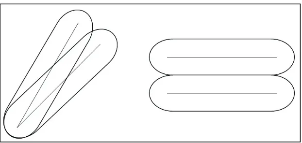
4 USING CAPSULE TO MODEL A LINK

It is easy to see that a link will be damaged when its distance from the center of the

disaster is less than or equal to r. We define an area around the link, the occurrence of disaster

within which, will affect the link. The area is capsule shaped such that the distance between the

link and each of the parallel sides of the capsule is equal to r and the two parallel lines are joined

on the same side by a semi circle with center at the corresponding endpoint of the link and

having a radius ‘r’. This area will be called a capsule from now on. The capsule is shown in

figure 3.

Figure 3. Capsule

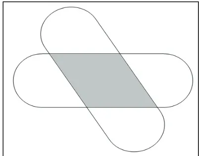
The part of the network worst affected by the disaster should lie in one of the intersections of the

capsules so formed. In the figure 4, the shaded region is more affected than any of the other

regions formed.

5 ASSESSING PLANAR NETWORKS

A network can be represented as either a planar graph or a non-planar graph. The

approach discussed in this section transforms any of the two types of network representations

into a planar graph using capsules. The resulting algorithm can be applied to both kinds of

networks. However, the algorithm has a lesser running time on planar networks. The non-planar

case of network is dealt in a different way in the next section.

A graph is planar if it can be drawn in the plane without any edges crossing. A formal

definition of a planar graph is as follows:

A graph is planar if there exists an embedding of the vertices in R2_{, f: V  R}2_{and a}

mapping of edges e Є E to simple curves in R2, fe: [0, 1]  R2 such that the endpoints of the

curves are the vertices at the endpoints of the edge, and no two curves intersect except possibly

at their endpoints.

A planar graph divides the plane into regions or faces. There is always exactly one

infinite region since a finite graph must occupy a finite portion of the plane. The number of

regions that the planar graph has is given by Euler’s formula.

5.1 EULER’S FORMULA

Euler's formula states that if a finite, connected, planar graph is drawn in the plane

without any edge intersections, and

• v is the number of vertices,

• e is the number of edges and

• f is the number of faces (regions bounded by edges, including the outer, infinitely-large

region), then

In terms of f,

f = e – v + 2 (2)

Figure 5 shows a simple example of a plane satisfying Euler’s formula.

Figure 5. Planar Graph

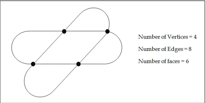
In our approach, the given network is represented by a planar graph P = (V, E) with

vertices v corresponding to the points of intersections of the boundaries of the capsules and

edges connect pairs of adjacent intersection points along the boundaries of the capsules. The

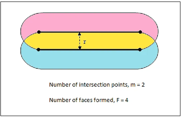
number of faces thus formed satisfies Euler’s formula. This is illustrated in figure 6.

The number of faces formed in terms of the intersection points is given by the following

theorem:

Theorem 2 [3]: Let m be the number of points of intersection of boundaries of the capsules, then

the number of faces f in the graph P is at most m + 2.

f = m + 2 (3)

Proof [3]: The proof is based on Euler’s formula for planar graphs. Since P = (V, E) is a planar

graph, |V| - |E| + |F| = 2, where V, E, F are the sets of vertices, edges, and faces of P,

respectively. If several boundaries intersect at the same point, then by slightly changing

boundaries, one can increase the number of faces. Thus for counting purposes, we can assume

that each point can be intersection of boundaries of at most two capsules. Then each vertex of the

graph P has degree 4. If we sum up degrees of all vertices, then we count each edge twice,

therefore, |E| = 2|V|. Thus, |V| - 2|V| + |F| = 2 and the number of faces equals |F| = |V| + 2.

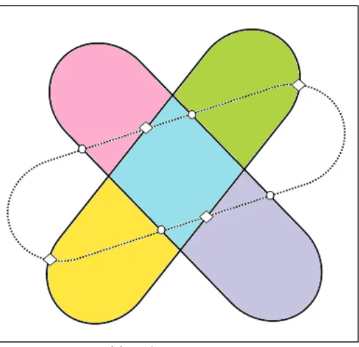
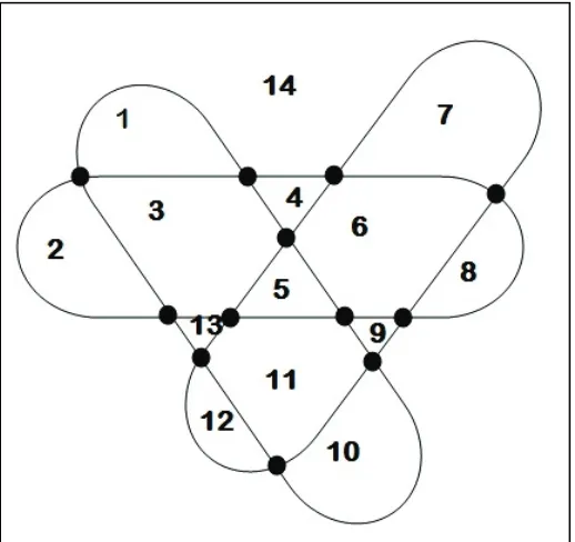
As an example figure 7 contains 3 capsules intersecting with each other. The number of

intersection points is 12 and the number of regions formed is 14, conforming to the theorem.

Figure 8 shows the faces for 3 non-parallel links.

Figure 8. Faces formed in case of non-parallel links

Figure 9 shows the faces formed in case of parallel links. Also, in the figure the distance

between the links is equal to the radius of the disaster.

6 WORST HIT FACE FOR PLANAR GRAPH (WHF-PG) ALGORITHM

To identify the most vulnerable part of the network, we propose the Worst Hit Face for

Planar Graph (WHF-PG) algorithm.

Algorithm Worst Hit Face for Planar Graph (WHF-PG)

1: input: r, radius of cut 2: for every link (i, j)

3: Draw a capsule, C of size r, around the link. 4: for every capsule, C

5: Find the intersection of C with its neighbors.

6: Define the faces

7: for every face, f

8: Evaluate the capacity of all links inside face f. 9: return face fmax with the maximum calculated capacity

As the algorithm indicates the face with the highest capacity, fmax is the worst hit region

of the network for the given disaster radius r.

6.1 COMPLEXITY

The number of nodes in the network is N. The number of links that can be formed with

these nodes cannot exceed N2. Since one capsule is drawn per link, their number is also of the O

(N2_{). Two capsules can intersect only at a node. A face is formed at every node and around every}

edge. So, the number of faces formed is equal to the sum of the nodes and edges in the graph.

Hence, the number of faces is O (N2_{). Summing the capacity of links in every face takes O (N}2_).

7 ASSESSING NON-PLANAR NETWORKS

The WHF-PG algorithm is more suitable for networks which don’t contain link

intersections. But a real world wired network contains numerous links passing over the same

points and links which are not connected to other links but are a part of the network. The number

of capsules as before is equal to the number of links and is of O (N2) where N is the number of

nodes in the network. The number of link intersections can potentially be of O (N4_{). Applying}

the Euler’s formula, we see that the number of faces formed is of O (N4_{). Evaluating the capacity}

of each face takes O (N2) time. This makes the running time of the WHF-PG algorithm of O

(N6_{). A faster algorithm can be produced by making use of the plane sweep technique. Before}

discussing this approach we present an alternative formula for finding the number of faces

formed by the intersection of capsules. This number is in terms of the capsules in contrast to the

Euler’s formula which gives the number of faces formed in terms of the number of intersection

points of capsules and the edges joining those intersection points.

Regions are formed by the intersection of capsules in combinations of 2, 3, 4…N2_{. For}

example, in figure 10, region A is formed by the intersection of capsules numbered 1 and 2.

Region B is formed by capsules 1, 2 and 3. Region C is formed by capsules 1, 2, 3 and 4. So, it is

seen that a region formed by any combination of the capsules can be a candidate for the most

affected area. Further, the sum of these combinations is exponential. This gives us an impression

Figure 10. Regions formed by capsule intersection

However, a very important observation made in reference [4] with respect to the Venn

diagrams dispels this notion and shows that the total number of regions is polynomial and is in

fact of O (N2_{) where N is the number of circles. We extend the same logic to capsules and show}

that only a polynomial number of regions need to be considered to find a region of the network

with maximum capacity.

[4] discusses an issue related to Venn diagrams. Venn diagrams are used to teach elementary

set theory, as well as illustrate simple set relationships in probability, logic, statistics, linguistics

and computer science. Typically we draw Venn diagrams to visualize the intersections among

two or three sets. We rarely come across Venn diagrams representing four sets. This is because

the task of arranging four circles is not as straightforward as it is in the case of fewer sets. Trying

to arrange four circles to represent all possible combinations is practically impossible with Venn

diagrams. It can however be done with other shapes. But our interest is only in the congruent

circles. [4] attempts to answers two questions in this regard:

1. How many regions must a Venn diagram have in order to display all the possible

intersections among n sets?

The answer to the first question is well known - a Venn diagram for n component sets must

contain all 2n _{hypothetically possible zones corresponding to some combination of being}

included or excluded in each of the component sets.

The second question is solved as follows: To maximize the number of regions, we make sure

no more than two circles intersect at a given point. Let rn denote this maximum number. Now

suppose we have n -1 circles drawn already with a total rn-1 regions. How many more regions can

the addition of one more circle yield? To maximize the number of regions, we draw the nth _circle

so that it intersects the existing n - 1 circles in two distinct points each (nonintersecting and

tangent circles produce no new regions). When the nth circle intersects an existing circle, it

creates two new regions: it begins one new region when it enters the existing circle, and starts

another upon leaving the circle. See figure 11.

The above analysis demonstrates that rn = rn-1 + 2(n-1). For large values of n, the

following substitutions and computations in figure 12 demonstrate that rn = n2 – n + 2. We see

that n2 _{– n + 2 = 2}n _{for n = 1, 2, 3, but n}2 _{– n + 2 < 2}n _{for n ≥ 4. There is immense reduction in the}

number of regions formed as compared to the number of regions that are supposed to be formed.

Figure 12. An explicit formula for the maximum number of regions formed by n circles [4]

Applying the same reasoning to the capsules, we observe that one capsule intersects

another capsule at a maximum of 4 points to form a maximum of 4 additional regions. There are

cases where the boundaries of the capsules overlap along the arcs or straight edges where the

entire segment forms the set of intersection points. These cases (figure 13) can be safely ignored

Figure 13. Capsules intersecting along boundaries

Theorem 3: The number of regions formed by the intersection of n capsules is of the order n2_.

Proof: It is easy to prove analytically that two capsules that do not have a part of their boundary

in common cannot meet at more than four points. The scenarios in which two capsules intersect

along an arc or a line are of little interest to us as they don’t form regions. If they should be

considered, it is enough to count only the endpoints of these overlapping line segments when

trying to define regions.

Suppose there are n-1 capsules and Rn-1 regions already existing. We add an nth capsule.

Since, the nth capsule intersects every existing capsule at a maximum of four points, the total

number of intersection points is 4*(n-1). The line or curve joining any consecutive pair of

intersection points belongs to the nth _{capsule’s boundary. This line (or curve) lies completely in}

exactly one existing region. This implies that there is one existing region corresponding to every

pair of consecutive intersection points. For each region that a line of the capsule goes through, it

adds a region (splits the region into 2 regions). Hence, the number of new regions formed by the

introduction of a new capsule is at most 4*(n-1) and the maximum total number of regions is at

Figure 14. Proof for Theorem 3

Figure 15 shows the substitutions and computations to arrive at an explicit formula for

the maximum number of regions formed by the intersecting capsules.

The formula gives the maximum number of regions formed in terms of the capsule

number, n. The formula in turn provides an upper bound on the worst-case time complexity of

the problem of finding the most affected region. For N nodes in the network, the number of

capsules would at most be O (N2). Applying the formula, the number of regions formed is found

to be of O (N4_{). The evaluation of each of these regions to find the worst affected region results}

in a running time of O (N6_{). This is the time taken if every region had to be evaluated naively in}

the worst-case scenario.

7.1 PLANE SWEEP TECHNIQUE

The main reason for using the capsules in this work is to mark the affected regions precisely. The

fact that still stands is that the worst affected regions lie around the points of link intersections.

Hence, we need an efficient approach to find these intersection points. In this section we

introduce one such algorithm called the plane sweep algorithm [34] which will prove to be a

useful technique in assessing the effect of disasters on non planar networks. Plane-sweep is an

algorithm schema for two-dimensional geometry of great generality and effectiveness. It works

for a surprisingly large set of problems, and when it works, tends to be very efficient. The

closely related Bentley–Ottmann algorithm uses the plane sweep technique to report

all K intersections among any N segments in the plane in time complexity of O((N + K) log N)

The feature of the technique is that intersection points of the originally given segments are found

during the sweep and considered as forthcoming tasks. No back-tracking is needed and no

intersecting points are left discovered. Another positive feature of plane sweep is that it is

output-sensitive i.e., its running time is output-sensitive to the number of intersection points, making it faster on

time when compared to the straight forward approach of checking every pair of lines for

intersection which takes O (N4_{) time.}

We now discuss the plane sweep algorithm in detail. Let S = s1, s2, s3,…, sn denote the

line segments whose intersections we wish to compute. Here are the main elements of any plane

sweep algorithm, and how we will apply them to this problem:

Sweep line: The name plane-sweep is derived from the image of sweeping the plane from left to

right with a vertical line called the sweep line stopping at every transition point (event) of a

geometric configuration to update the cross section. We maintain the line segments that intersect

the sweep line in sorted order (say from top to bottom).

Events: Although we might think of the sweep line as moving continuously, we only need to

update data structures at points of some significant change in the sweep-line contents, called

event points.

Different applications of plane sweep will have different notions of what event points are. For

this work, event points will correspond to the following:

Endpoint events: where the sweep line encounters an endpoint of a line segment, and

Intersection events: where the sweep line encounters an intersection point of two line segments.

Note that endpoint events can be presorted before the sweep runs. In contrast, intersection events

will be discovered as the sweep executes. For example, in the figure 16, some of the intersection

points lying to the right of the sweep line have not yet been “discovered” as events. However, we

will show that every intersection point will be discovered as an event before the sweep line

Figure 16. Intersection Events [7]

Event updates: When an event is encountered, we must update the data structures associated

with the event. It is a good idea to be careful in specifying exactly what invariants you intend to

maintain. For example, when we encounter an intersection point, we must interchange the order

of the intersecting line segments along the sweep line.

Degeneracies: There are a great number of special cases that complicate the algorithm and

obscure the main points. We will make a number of simplifying assumptions. They can be

overcome through a more careful handling of these cases.

(1) No line segment is vertical.

(2) If two segments intersect, then they intersect in a single point (that is, they are not collinear).

(3) No three lines intersect in a common point.

Detecting intersections: We mentioned that endpoint events are all known in advance. But how

do we detect intersection events. It is important that each event be detected before the occurrence

of the actual event. The strategy used is as follows. Whenever two line segments become

right of the sweep line. If so, we will add this new event (assuming that it has not already been

added). A natural question is whether this is sufficient. In particular, if two line segments do

intersect, is there necessarily some prior placement of the sweep line such that they are adjacent.

Interestingly, this is the case, but it requires a proof. The lemma from [7] proves this.

Lemma: Given two segments si and sj , which intersect in a single point p (and assuming no

other line segment passes through this point) there is a placement of the sweep line prior to this

event, such that si and sj are adjacent along the sweep line (and hence will be tested for

intersection).

Proof: From our general position assumption it follows that no three lines intersect in a common

point. Therefore if we consider a placement of the sweep line that is infinitesimally to the left of

the intersection point, lines si and sj will be adjacent along this sweep line L. Consider the event

point q with the largest x-coordinate that is strictly less than px. The order of lines along the

sweep-line after processing q will be identical along the sweep line just prior p, and hence si and

sj will be adjacent at this point (Figure 17)

Data structures: In order to perform the sweep we will need two data structures.

1. Event queue: This holds the set of future events, sorted according to increasing x-coordinate.

Each event contains the auxiliary information of what type of event this is (segment endpoint or

intersection) and which segment(s) are involved. The operations that this data structure should

support are inserting an event (if it is not already present in the queue) and extracting the next

event. The x-queue must be a priority queue; it can be implemented as a heap. If events have the

same x-coordinate, then we can handle this by sorting points lexicographically by (x, y). (This

results in events being processed from bottom to top along the sweep line). The cost of inserting

or getting the next element can be performed in O (log n) time each.

2. Sweep line status: To store the sweep line status, we maintain a balanced binary tree whose

entries are pointers to the line segments, stored in increasing order of y-coordinate along the

current sweep line. The operations that we need to support are those of deleting a line segment,

inserting a line segment, swapping the position of two line segments, and determining the

immediate predecessor and successor of any item. Assuming any balanced binary tree, these

operations can be performed in O (log n) time each.

The Algorithm: The complete plane-sweep algorithm is presented in figures 18 and 19. Figure

Figure 18. Plane Sweep Algorithm [34]

Figure 19. Plane Sweep Algorithm (contd.)

Figure 20. Sweep line status

Analysis: The work done by the algorithm is dominated by the time spent updating the various

data structures (since otherwise we spend only constant time per sweep event). We need to count

two things: the number of operations applied to each data structure and the amount of time

needed to process each operation.

For the sweep line status, there are at most n elements intersecting the sweep line at any time,

and therefore the time needed to perform any single operation is O(log n), from standard results

on balanced binary trees. Since we do not allow duplicate events to exist in the event queue, the

total number of elements in the queue at any time is at most (2n + I). Since we use a balanced

binary tree to store the event queue, each operation takes time at most logarithmic in the size of

the queue, which is O (log (2n + I)). Since I ≤ n2_{, this is at most O (log n}2_{) = O (2 log n) = O (log}

n) time. Each event involves a constant number of accesses or operations to the sweep status or

the event queue, and since each such operation takes O (log n) time from the previous paragraph,

it follows that the total time spent processing all the events from the sweep line is

O ((2n + I) log n) = O ((n + I) log n) = O(n log n + I log n) (4)

7.2 MODIFIED PLANE SWEEP TO IDENTIFY REGIONS

We now discuss modifications to the plane sweep algorithm so that it can be a suitable

solution to our problem of finding the most affected region of the network. Evidently, the regions

around line intersections or regions in which lines lie close to each other are more affected than

regions containing single links. Hence, the first step in finding the region most affected should be

to find link intersections. We can then find the region formed by the overlapping of

corresponding capsules to get the worst hit region we are looking for. The plane sweep algorithm

is an output sensitive algorithm whose running time depends on both the input and the output.

This feature of the algorithm makes it suitable to be used in our problem. However, we have to

consider the degeneracies of the algorithm and additional scenarios in our problem that are not

considered in the basic plane sweep algorithm. The following sub sections discuss the

approaches taken to deal with the degeneracies. The changes that are to be made on the data

structures are discussed simultaneously.

7.2.1 VERTICAL LINES

The basic plane sweep algorithm assumes for simplicity that the graph doesn’t contain

any vertical line segments. In our problem, it is necessary for the vertical segments to have their

vertices processed. We can avoid the special treatment of these degeneracies. The sweep line

can be imagined to be “almost” vertical, that is, it forms a counterclockwise angle of infinitely

small value with the vertical line, as shown in figure 21. With this approach for vertical segments

the vertex of lower y-coordinate will be the left endpoint or source, thus imposing a

Figure 21. Handling vertical lines in plane sweep algorithm [10]

7.2.2 MULTIPLE INTERSECTIONS

In case of multiple intersections, the idea is to forbid the insertion of several points

having the same coordinates but belonging to different pairs of intersecting segments in the event

queue. The only point stored will mark the intersection between the upmost and the lowest

segments that intersect at the point. However, all line segments incident at the intersection point

should be stored with the event in order to fetch the corresponding capsules when finding the

region of intersection. Hence, the event point will now be associated with a set of line segments.

This set will be called the pencil.

Since any event can be a point of multiple line segment intersection, the pencil at an

existent intersection point has to be updated every time a new segment is found to intersect at

that point, An example is depicted in figure 22 (a). Here after processing the left endpoints of s1

and s2, an intersection point is detected and inserted in the event queue. When the algorithm

processes s3, it also detects the intersection with s3; the already existent intersection point (s1, s2)

will be replaced by (s1, s3) and the event’s pencil will be updated to (s1, s2,s3). In situations like

that depicted in figure 22 (b) the event queue keeps only the intersection (s1, sk). The event’s

Figure 22. Handling multiple intersections in plane sweep [10]

The sweep line status should be modified as follows:

i. Insertion: A line segment is inserted when its left point is encountered. After insertion the

segment must be tested against its neighbors in the line status and their eventual

intersection points will be inserted in the event queue.

ii. Deletion: A line segment is deleted from the sweep line status when the sweep line

encounters the line’s right endpoint. At this event, the former neighbors of the deleted

line segment are checked for intersection. If they intersect, then their intersection point is

stored in the event queue.

iii. Swapping: When an intersection event point is reached the segments that intersect here

must change place in the structure. This operation is followed by testing these segments

against their new neighbors and by inserting their eventual intersections that lie to the

right of the current event point in the event queue. If there exists a pencil of segments

sharing the current event they form a contiguous sequence of elements in the line status.

This sequence is bounded by the two segments that are associated to the event. At the

right of the intersection point the order of line segments in the pencil in the line status is

7.2.3 DANGLING LINKS

We use the term dangling to describe those edges of the network which are a part of the

network but are not connected any other link. They may lie close to a link or a link intersection

and have a possibility of being affect by the same disaster that affects their close link or link

intersection. It is therefore necessary to consider such links also during the evaluation. But, such

lines cannot be detected by the naïve plane sweep algorithm. We try to make use of a variation of

the plane sweep algorithm which is used to solve the closest pair problem.

When a new point p is encountered we wish to answer the question whether this point lies

at a distance less than or equal to r to one of the points on its left. All candidates lie in a half

circle centered at p, with radius r, where r is the radius of the disaster.

The key question to be answered in striving for efficiency is how to retrieve quickly all

the points seen so far that lie inside this half circle to the left of p, in order to compare their

distance to p. A rectangle query can be answered more efficiently. Thus we replace the

half-circle query with a bounding rectangle query, accepting the fact that we might include some

Figure 23. Bounding rectangle [9]

The event queue, as in the basic algorithm stores the points of the set S, ordered by their

x-coordinate, as events to be processed when updating the vertical cross section. We introduce

two pointers into the event queue, 'tail' and 'current', which partition S into four disjoint subsets:

i. The discarded points to the left of 'tail' are not accessed any longer.

ii. The active points between 'tail' (inclusive) and 'current' (exclusive) are being queried.

iii. The current transition point, p, is being processed.

iv. The future points have not yet been looked at.

The rectangle query in figure 23 is implemented in two steps. First, we cut off all the

points to the left at distance ≥ r from the sweep line. These points lie between 'tail' and 'current'

in the event queue and can be discarded easily by advancing 'tail' and removing them from the

event queue. Second, we consider only those points q in the r-slice whose vertical distance from

p is less than r i.e., |qy – py| < r. These points can be found in the sweep line status by looking at

8 WORST HIT FACE FOR NON PLANAR GRAPHS (WHF-NPG) ALGORITHM

We now present the Worst Hit Face for Non Planar Graphs (WHF-NPG) algorithm which

incorporates the handling of all scenarios discussed in the previous section to detect the worst hit

face in the given non planar graph.

Algorithm Worst Hit Face for Non Planar Graph (WHF-NPG)

Input: A set of line segments which represent the links in a non-planar graph Radius of disaster, r

Output: A region most affected by a disaster of radius r

Data Structures:

• Event Queue, Q is a priority queue which contains the events to be processed and past events that lie in the r-slice

• Pointers ‘tail’ and ‘current’. The current pointer points to the current event being processed. The interval between these two pointers contains the events that have been processed and whose distance from the current pointer ≤ r

• Sweep line status structure, T is a balanced tree which contains pointers to line segments, stored in increasing order of y-coordinate along the current position of the sweep line

• Every event point has a list of line segments that intersect at it. This list is called the pencil.

procedure findIntersections ()

1. capacityOfWHF  0, worstHitRegion 2. initQ(); initT()

3. while Q not empty

4. do p = nextQ()

5. handleEventPoint (p)

procedure handleEventPoint (Event p)

1. if ( leftEndPoint (Event p) ) 2. s := segment (p)

3. pencil := updatePencil (s, p) 4. insertT(s)

5. if (q = intersect (predT(s), s) or intersect(s, succT(s))) 6. insertQ (q)

7. pencil := updatePencil (s, q)

8. pastList := getPastEventsInBoundingBox() 9. defineRegion(pencil, pastList)

10. elseif ( rightEndPoint (Event p) ) 11. s := segment (p)

12. deleteT(s)

13. if (q = intersect (predT(s), succT(s))) 14. insertQ (q)

15. pencil := updatePencil (predT(s), q) 16. pencil := updatePencil (succT(s), q) 17. pastList := getPastEventsInBoundingBox() 18. defineRegion(pencil, pastList)

19. else /* p is an intersection point */

20. (s1, s2) := segments (p) /* Assume s1 is above s2 */

21. reverseT(s1, s2) /* reverse the order of segments between s1 and s2 */ 22. if ( q = intersect (predT(s2), s2) )

23. insertQ (q)

24. pencil := updatePencil (s2, q) 25. if ( q = intersect ( intersect (s1, succT(s1)) ) 26. insertQ (q)

27. pencil := updatePencil (s1, q)

procedure updatePencil (Segment s, Event p)

1. Add the segment s to the list of segments associated with the event point p

end updatePencil

procedure getPastEventsInSlice (Event p)

1. Returns the list of line segments associated with past events from event queue Q, which lie in the slice between pointer tail and event p

2. Returns predecessors and successors of point p on the sweep line at vertical distance ≤ r

end getPastEventsInSlice.

procedure defineRegion (pencil, pastList)

1. capsules = Retrieve capsules corresponding to the links in pencil and pastList.

2. regionFormed = Find the region formed by the intersection of all capsules.

3. capacityOfFace = Sum (Capacity of links in pencil and pastList) 4. if (capacityOfFace ≥ capacityOfWHF)

5. capacityOfWHF = capacityOfFace 6. worstHitRegion = regionFormed

7. end if

end defineRegion

8.1 COMPLEXITY

The number of nodes in the non planar graph is N. The number of links is of O (N2_{). The}

number of link intersections is of O (N4_{) and the number of regions is of O (N}4_{). The number of}

events that can be encountered by the sweep line is equal to the sum of the number of endpoints

and the number of intersection points, which is O (N4_).

The operations 'insertT' and 'deleteT' on the sweep line status T are performed in O (log

N2_{) time, and 'succT' and 'predT' are performed in O(1). The event queue Q is a priority queue}

that supports the operation 'insertQ'; it can be implemented as a heap. The cost for initializing the

requirement of the x-queue is O (N +N4_{), which implies that the cost for calling 'insertQ' and}

'nextQ' is O (log N4_{). The cost for reversing the order of line segments in the sweep line status is}

O (log N2_{). The time taken to get the past events is reduced as a result of using the two pointers}

‘tail’ and ‘current’ in the event queue. The retrieval of the past events with respect to the current

event along both the x and y coordinates can be done in O (log N4_).

The O (log N4_{) operations on event queue Q and sweep line status are executed at each of}

the endpoints and intersection points. Therefore, the running time of the algorithm is of

9 CONCLUSIONS

This work addressed a very important concern in the field of wired computer networks

and suggests novel ways to solve the problem. Algorithms have been proposed for both planar

and non-planar graphs. The WHF-PG algorithm for planar graphs can be applied to evaluate the

impact of disasters on transoceanic cables which are to a great extent planar in nature. The

WHF-NPG algorithm proposed for non planar graphs finds great usage in evaluating vulnerability of

networks in cities with high volume of interconnected fibers and backbone networks of an entire

country. The solution can be applied to other networks like telephone networks as well. The

knowledge of physical susceptibility helps in the redesigning of network so as to secure the

network as much as possible. One contribution of the work is to ascertain that the number of

regions or faces formed by the intersection of the capsules in terms of the number of capsules

which is of O (n2_{). The paper provides a proof for the same. The most important contribution of}

the paper is the application of plane sweep algorithm to the non planar network to determine the

faces. The running time of the proposed algorithm is O (N4 _{log N), which is less than that}

presented in the previous work. The algorithm can be easily implemented with well known

REFERENCES

[1] S. Neumayer, G. Zussman, R. Cohen, and E. Modiano, Assessing the Vulnerability of the

Fiber Infrastructure to Disasters, Submitted to IEEE/ACM Trans. on Networking

(preliminary version in IEEE INFOCOM'09).

[2] S. Neumayer, G. Zussman, R. Cohen, and E. Modia

[3] Berman, P., G. Calinescu, et al. (2004). Power efficient monitoring management in sensor

networks. Wireless Communications and Networking Conference, 2004. WCNC. 2004 IEEE

4: 2329 - 2334.

[4] Amy N. Myers. Are Venn Diagrams Limited to Three or Fewer Sets?

[5]

[6]

[7] Computational Geometry. David M. Mount, Department of Computer Science, University of

Maryland, Fall 2002

[8]

[9]

[10] Freiseisen W., and Pau, P. A generic plane-sweep for intersecting line segments,

Technical Report RISC-Linz TR-98-18, University of Linz, Linz, Austria, 1998.

[11] P. Agarwal, A. Efrat, A. Ganjugunte, D. Hay, S. Sankararaman, and G.

Zussman, Network Vulnerability to Single, Multiple, and Probabilistic Physical Attacks,

Proc. IEEE MILCOM'10, Nov. 2010.

[12] R. Bhandari, Survivable Networks: Algorithms for Diverse Routing, Kluwer Academic

[13] O. Gerstel and R. Ramaswami, "Optical layer survivability: A services perspective,"

IEEE Commun. Mag., vol. 38, no. 3, pp. 104-113, Mar. 2000.

[14] J. Manchester, D. Saha, and S. K. Tripathi (eds.), "Protection, restoration, and disoster

recovery," IEEE Network, Special issue, vol. 18, no. 2, Mar.-Apr. 2004.

[15] D. Zhou and S. Subramaniam, “Survivability in optical networks”, IEEE Network, vol.

14, pp. 16–23, 2000.

[16] E. Modiano, A. Narula-Tam, “Survivable Lightpath Routing: A New Approach to the

design of WDM-Based Networks”, IEEE Journal on Selected Areas in Communications, vol.

20, no. 4, May 2002.

[17] A. Narula-Tam, E. Modiano and A. Brzezinski, “Physical Topology Design for

Survivable Routing of Logical Rings in WDM-Based Networks”, MIT LIDS Technical

Report P-261, July 2003.

[18] C. A. Phillips. The network inhibition problem. In STOC ’93: Proceedings of the

twentyfifth annual ACM symposium on Theory of computing, pages 776–785, New York,

NY.

[19] A. Pinar, Y. Fogel, and B. Lesieutre, “The inhibiting bisection problem,” in Proc. ACM

SPAA’07, 2007. USA, 1993. ACM Press.

[20] R. L. Church, M. P. Scaparra, and R. S. Middleton, “Identifying critical infrastructure:

the median and covering facility interdiction problems,” Ann. Assoc. Amer. Geographers,

vol. 94, no. 3, pp. 491–502, 2004.

[21] D. Bienstock, “Some generalized max-flow min-cut problems in the plane,” Math. Oper.

[22] R. Cohen, K. Erez, D. Ben-Avraham, and S. Havlin, “Resilience of the Internet to

random breakdowns,” Phys. Rev. Lett., vol. 85, pp. 4626–4628, Nov. 2000.

[23] R. Cohen, K. Erez, D. Ben-Avraham, and S. Havlin, “Breakdown of the Internet under

intentional attack,” Phys. Rev. Lett., vol. 86, no. 16, pp. 3682–3685, Apr 2001.

[24] L. K. Gallos, R. Cohen, P. Argyrakis, A. Bunde, S. Havlin, “Stability and topology of

scale free networks under attack and defense strategies,” Phys. Rev.Lett., vol. 94, no. 18,

2005

[25] D. Magoni, “Tearing down the Internet,” IEEE J. Sel. Areas Commun., vol. 21, no. 6, pp.

949–960, Aug. 2003.

[26] A. L. Barabasi and R. Albert, “Emergence of scaling in random networks,” Science, vol.

286, no. 5439, pp. 509–512, October 1999.

[27] P. Francis, S. Jamin, C. Jin, Y. Jin, D. Raz, Y. Shavitt, and L. Zhang, “IDMaps: A global

Internet host distance estimation service,” IEEE/ACM Trans. Netw., vol. 9, no. 5, pp. 525–

540, October 2001.

[28] S. Bar, M. Gonen, and A. Wool, “A geographic directed preferential Internet topology

model,” in Proc. IEEE MASCOTS’05, Sept. 2005.

[29] A. Lakhina, J. Byers, M. Crovella, and I. Matta, “On the geographic location of Internet

resources,” IEEE J. Sel. Areas Commun., vol. 21, no. 6, pp. 934–948, 2003.

[30] S. Yook, H. Jeong, and A. Barabasi, “Modeling the Internet’s large-scale topology,”

Proc. Natl. Acad. Sci., vol. 99, no. 21, pp. 13 382–13 386, 2002

[31] C. P. Warren, L. M. Sander, and I. M. Sokolov, “Geography in a scale-free network

[32] H. Yukio and J. Matsukubo, “A review of recent studies of geographical scale-free

networks,” Trans. Inf. Process. Society of Japan, vol. 47, no. 3, pp. 776–785, 2006

[33] J. S. Foster Jr. et al., “Report of the commission to assess the threat to the United States

from electromagnetic pulse (EMP) attack, Vol. I: Executive report,” Apr. 2004.

[34] Computational geometry: algorithms and applications by Mark de Berg, Otfried Cheong,

Marc van Kreveld, Mark Overmars

[35] Fiber-Optic and Satellite Communications by Gilbert Held

[36] What are the advantages of Wired Networking? [Online] Available:

[37] Ranjitha Shivarudraiah., “STCP: A new transport protocol for high-speed networks,”