Georgia State University Georgia State University
ScholarWorks @ Georgia State University
ScholarWorks @ Georgia State University
Sociology Dissertations Department of Sociology
Fall 11-17-2011
HOV to the MD? A Multilevel Analysis of Urban Sprawl and the
HOV to the MD? A Multilevel Analysis of Urban Sprawl and the
Risk for Negative Health Outcomes
Risk for Negative Health Outcomes
William Mark Sweatman Ph.D.
Georgia State University
Follow this and additional works at: https://scholarworks.gsu.edu/sociology_diss
Part of the Sociology Commons
Recommended Citation Recommended Citation
Sweatman, William Mark Ph.D., "HOV to the MD? A Multilevel Analysis of Urban Sprawl and the Risk for Negative Health Outcomes." Dissertation, Georgia State University, 2011.
https://scholarworks.gsu.edu/sociology_diss/61
This Dissertation is brought to you for free and open access by the Department of Sociology at ScholarWorks @ Georgia State University. It has been accepted for inclusion in Sociology Dissertations by an authorized
HOV TO THE MD?
A MULTILEVEL ANALYSIS OF URBAN SPRAWL
AND THE RISK FOR NEGATIVE HEALTH OUTCOMES
by
WILLIAM MARK SWEATMAN
Under the direction of Dawn Baunach, Ph.D.
ABSTRACT
Urban sprawl often has a negative connotation, used as a derogatory label for
certain forms and consequences of land development that are seen as environmentally
and socially unpleasant. Although sprawl may be seen as offensive, there may be other,
far greater and more harmful consequences of sprawl. The literature indicates that rates
of negative health outcomes, such as obesity, tend to be higher in more developed areas.
However, aside from a few studies, little empirical research looks specifically at the
influence of sprawl when it comes to individual health. This research project focuses on
sprawl and examines the relationships it has with health behaviors and health outcomes.
By analyzing data from the CDC’s 2003 Behavioral Risk Factor Surveillance System
self-reported and calculated variables, I investigate the associations between sprawl, physical
activity, body weight, and health outcomes using Structural Equation Modeling (SEM).
By employing SEM, my research differs from previous research in this field by adding
not only additional layers to the evaluation of sprawl and health outcomes, but also
allows for the evaluation of associations through various “paths” instead of looking at
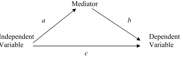
variables within simpler hierarchical regression models. In addition to direct effects, it
also allows for the determination of indirect, or mediated, effects between variables
within a path model. Even though no direct relationship between sprawl and health
outcomes was revealed, sprawl did show to have a statistically significant indirect effect
on health outcomes mediated by physical activity and body weight. Physical activity is
also shown to mediate the relationship between sprawl and body weight. Additionally,
physical activity reveals both a direct and indirect effect on health outcomes, with its
indirect effect being mediated by body weight. Finally, physical activity and body
weight are both shown to have statistically significant direct effects on health outcomes.
In the concluding chapter I propose a new path model in light of the results of the
analyses of data in order to represent the associations between sprawl, physical activity,
body weight, and health outcomes more accurately.
HOV TO THE MD?
A MULTILEVEL ANALYSIS OF URBAN SPRAWL
AND THE RISK FOR NEGATIVE HEALTH OUTCOMES
by
WILLIAM MARK SWEATMAN
A Dissertation Submitted in Partial Fulfillment of the Requirements for the Degree of
Doctor of Philosophy
in the College of Arts and Sciences
Georgia State University
Copyright by William Mark Sweatman
HOV TO THE MD?
A MULTILEVEL ANALYSIS OF URBAN SPRAWL
AND THE RISK FOR NEGATIVE HEALTH OUTCOMES
by
WILLIAM MARK SWEATMAN
Committee Chair: Dawn Baunach, Ph.D.
Committee: Charlie Jaret, Ph.D.
Mary Ball, Ph.D.
Electronic Version Approved:
Office of Graduate Studies
College of Arts and Sciences
Georgia State University
DEDICATION
To my parents, thank you so much for the social and financial capital you have
given me. Without the resources you blessed me with I would never have been able to
achieve the dream of obtaining my doctorate. And even more so, thank you so much for
the love you have given me throughout the years. I love you both so very much. Thank
ACKNOWLEDGEMENTS
I would like to thank the chair of my committee, Dr. Dawn Baunach, for all of her
advice and support. Her knowledge of quantitative sociology provided me with great
guidance during my dissertation journey. I also would like to thank my committee
members, Dr. Charlie Jaret and Dr. Mary Ball, for their constructive criticism and
knowledge of sociological matters. My dissertation is well-rounded and impressive due
to the guidance and advice from my entire dissertation committee.
I would like to thank Dr. Molly Perkins and Dr. Mignon Montpetit for their expert
knowledge of multilevel statistical analysis and their unwavering support and
encouragement.
I would also like to thank my colleagues for their encouragement and support
during graduate school, especially Pam Regus, Josie Parker, Evelina Sterling, Linda
Danavall, and Emmie Cochran-Jackson. Each of you has made the journey through the
TABLE OF CONTENTS
ACKNOWLEDGEMENTS ... V
LIST OF TABLES ...IX
LIST OF FIGURES ... X
CHAPTER 1
INTRODUCTION ... 1
CHAPTER 2 REVIEW OF THE LITERATURE... 6
PHYSICAL ACTIVITY AND HOW IT RELATES TO WEIGHT AND HEALTH... 6
SUBURBANIZATION AND HOW IT RELATES TO PHYSICAL ACTIVITY... 8
STUDIES LOOKING AT SPRAWL AND HEALTH... 12
CHAPTER 3 CONCEPTUAL FRAMEWORK ... 15
HYPOTHESES... 18
ADDITIONAL CONSIDERATIONS... 20
CHAPTER 4 MEASURES OF URBAN SPRAWL... 22
STUDIES FOCUSING ON SPRAWL AND HEALTH OUTCOMES... 23
CONCLUSION... 27
CHAPTER 5 METHODOLOGY ... 29
CONTROL VARIABLES... 37
SOCIODEMOGRAPHIC CONTROL VARIABLES... 37
PERSONAL HEALTH CONTROL VARIABLE... 41
REGIONAL CONTROL VARIABLE... 43
ANALYTIC TECHNIQUE... 43
MODEL ANALYSES... 44
SIMILARITIES AND DIFFERENCE BETWEEN THIS STUDY AND EWING ET AL.STUDY... 49
LIMITATIONS... 50
FINDINGS... 52
CHAPTER 6 SPRAWL AND NEGATIVE HEALTH OUTCOMES ... 53
PREDICTION OF NEGATIVE HEALTH OUTCOMES WITH SPRAWL... 54
AGE,EDUCATION,INCOME, AND GENDER AS PREDICTORS OF NEGATIVE HEALTH OUTCOMES... 59
RACE AND ETHNICITY AS PREDICTORS OF NEGATIVE HEALTH OUTCOMES... 62
MARITAL STATUS AS PREDICTORS OF NEGATIVE HEALTH OUTCOMES... 64
PERSONAL HEALTH AS PREDICTORS OF NEGATIVE HEALTH OUTCOMES... 65
REGION AS A PREDICTOR OF NEGATIVE HEALTH OUTCOMES... 66
FIT STATISTICS... 67
SUMMARY... 69
CHAPTER 7 SPRAWL AND NEGATIVE HEALTH OUTCOMES WITH PHYSICAL ACTIVITY AND BMI AS MEDIATING VARIABLES INCLUDING ALL HYPOTHESIZED PATHS ... 71
PREDICTION OF PHYSICAL ACTIVITY... 72
PREDICTION OF BODY MASS INDEX (BMI)... 75
PHYSICAL ACTIVITY AND BMI AS INDEPENDENT VARIABLES... 77
INDIRECT EFFECT OF SPRAWL THROUGH PHYSICAL ACTIVITY ON NEGATIVE HEALTH OUTCOMES,PATHS
H1 AND H6 ... 82
INDIRECT EFFECT OF SPRAWL THROUGH BMI ON NEGATIVE HEALTH OUTCOMES,PATHS H4 AND H3 ... 83
INDIRECT EFFECT OF SPRAWL THROUGH PHYSICAL ACTIVITY AND BMI ON NEGATIVE HEALTH OUTCOMES,PATHS H1,H2, AND H3... 84
INDIRECT EFFECT OF PHYSICAL ACTIVITY THROUGH BMI ON NEGATIVE HEALTH OUTCOMES,PATHS H2 AND H3 ... 85
INDIRECT EFFECT OF SPRAWL THROUGH PHYSICAL ACTIVITY ON BMI,PATHS H1 AND H2 ... 85
CHAPTER 8 DISCUSSION AND CONCLUSION ... 86
VALIDITY OF HYPOTHESES... 86
ASSOCIATIONS BETWEEN VARIABLES IN THE CONCEPTUAL MODEL... 92
BEST FITTING ANALYTICAL MODEL... 94
PROPOSAL OF A NEW CONCEPTUAL MODEL... 95
CONTRIBUTIONS TO THE LITERATURE... 97
IMPLICATIONS AT AN APPLIED LEVEL... 98
POSSIBILITIES FOR FUTURE RESEARCH... 99
CONCLUSION... 101
REFERENCES... 105
APPENDIX A... 112
LIST OF COUNTY-LEVEL SPRAWL INDEX, FIPS, AND REGION CLASSIFICATION ... 112
APPENDIX B ... 125
COUNTY SPRAWL INDEX VARIABLES ... 125
APPENDIX C... 126
LIST OF TABLES
Table 2.1 Central City Population and Job Loss ... 9
Table 5.1 Difference in Means Significance Testing ... 31
Table 5.2 Descriptive Statistics ... 32
Table 6.1 Zero-order Relationship between Sprawl and Negative Health
Outcomes... 56
Table 6.2 Baseline Model SEM Regression Results for Negative Health Outcomes. 57
LIST OF FIGURES
Figure 3.1 Established (Solid) and Speculative (Dashed) Relationships ... 17
Figure 3.2 Conceptual Model Used in this Dissertation ... 18
Figure 5.1 Analytical Model ... 46
Figure 5.2 Independent, Dependent, and Mediating Variables ... 47
Figure 6.1 Baseline Analytical Path Model ... 54
Figure 7.1 Analytical Path Model Two... 71
CHAPTER 1
INTRODUCTION
It is not uncommon for many people to associate urban sprawl with a negative
connotation, using the term as a derogatory label for certain forms and consequences of land
development that are seen as environmentally and socially unpleasant (Freeman 2001; Razin
1998; Wassmer 2002). Although many people may view sprawl as offensive, there may be
other, far greater and more harmful consequences of sprawl. The literature indicates that rates of
negative health outcomes, such as obesity, tend to be higher in areas that are more sprawling
(McCann and Ewing 2003; Kelly-Schwartz et al. 2004; Ewing et al. 2003). A recent study
supports this association indicating a relationship between urban sprawl and the risk for being
overweight or obese (Lopez 2004). Aside from a few studies, little empirical research looks
specifically at the influence of sprawl when it comes to the health of individuals. However,
urban sprawl is receiving growing attention, and the empirical evidence that does exist generally
supports links between built environmental conditions and health outcomes (Giles-Corti and
Donovan 2002).
Associations between the built environment and health are not new. In the late 19th
century, public health practitioners realized the effects of the built environment on the public;
how the very place where people lived and worked affected their health. Unsanitary sewage and
water conditions, dark airless tenement housing, and toxic industrial wastes all contributed to the
spread of disease. In response to such conditions, planners advocated public infrastructure, such
as water and sewer lines, building codes, and zoning plans to separate people from toxins and
influence public health. People who reside in sprawling suburban areas are now suffering from
chronic health conditions that earlier generations did not. The lack of physical activity, poor
diets, air pollutants, and environmental toxins may cause many people to suffer from chronic
health problems such as heart disease, asthma, and diabetes at rates previous generations did not
(Perdue 2004). It is just as important today, as it was over one hundred years ago, to understand
associations between the built environment and public health.
It has long been documented that body weight is associated with negative health
outcomes, such as diabetes, cardiovascular disease, and cancer, and that the risk of mortality
increases with the severity of obesity (Calle et al. 1999). Unfortunately, rates of obesity are
increasing rapidly in the United States (Flegal et al. 1998; Kuczmarski et al.1994; Bianchini,
Kaaks, and Vainio 2002). Obesity, and the plethora of diseases that come along with it, used to
be blamed on the fact that Americans eat too much fattening food. Although this may be true,
researchers now are focusing on another component of the crisis, that of low levels of physical
activity. It is well agreed upon that Americans are too sedentary and weigh too much (McCann
and Ewing 2003).
Decreasing body mass and maintaining a proper weight is a means to reduce the risks for
deadly diseases such as diabetes and heart disease, and one very important way to maintain a
healthy weight is to be physically active (Flegal, Carroll, Kuczmarski, and Johnson 1994).
Medical research has shown that walking and similar forms of moderate physical activity help
maintain a healthy weight. However, the lack of physical activity, as well as being overweight,
factor into more than 200,000 premature deaths annually. Therefore, it is very important for
individuals to be physically active in order to reduce their risk for obesity and its associated
physically active on a regular basis may pose a significant problem for those who reside in
sprawling areas.
Community form has a strong relationship to one’s health. The design of communities
influences health by encouraging or discouraging routine physical activity involved in daily life.
People living in sprawling areas, for example, may miss out on significant health benefits
available, such as walking to the store, to work, or other places as part of a daily routine
(McCann and Ewing 2003). Patterns of streets within neighborhoods, such as those found in
many suburban subdivisions, affect how people use their cars and their propensity to walk.
Metropolitan areas with high levels of urban sprawl tend to have higher per capita vehicle miles
traveled daily, even after controlling for factors such as income, size of metropolitan area, and
location within the nation. This suggests that people in high-sprawl areas drive more, quite
possibly at the expense of daily physical activity (Lopez 2004). This association between
development patterns and health outcomes can be seen as an indirect effect mediated by physical
activity and body weight.
Even though some research linking sprawl with health status exists, there is the need for
more empirical research on this relationship. This research project helps fill the need for
additional empirical measures by looking for associations between sprawl, physical activity,
weight, and disease. It specifically follows up on and refines the approach and results of Ewing
et al. (2003). It tests the relationship between all of these variables by focusing on a conceptual
model linking each variable via different hypotheses. It not only addresses the issue of how
sprawl relates to health outcomes, but also addresses the issue of how sprawl relates to physical
activity and weight. Various “paths” through the conceptual model allow me to determine which
disease, high cholesterol, hypertension, and stroke. These variables are outcomes in my
conceptual model because previous research shows they have a high association with a lack of
regular physical activity and body weight. Therefore, based on previous studies it is reasonable
to hypothesize that individuals who reside in more sprawling areas are more prone to have a
higher risk for such conditions because they are less likely to obtain the beneficial aspects of
regular daily physical activity due to the design of their built environment.
There are many questions that arise when looking for associations between sprawl and
health outcomes, such as: How does sprawl specifically affect health outcomes? Does
county-level sprawl have a direct association with individual-county-level health outcomes? Most likely not,
but it may have a direct effect on levels of individual physical activity. It is apparent from many
studies that weight gain does have a causal effect on health outcomes and that less physical
activity does affect weight (Calle et al. 1999; Flegal et al. 1998; Kuczmarski et al. 1994;
Bianchini et al. 2002; McCann and Ewing 2003; Mokdad et al. 2001), but what association, if
any, does a higher level variable like sprawl have on individual-level health?
This research project explores the questions listed above by focusing on sprawl and
determining relationships it has with physical activity, body weight, and specific health
outcomes. By analyzing data from the CDC’s Behavioral Risk Factor Surveillance System
(BRFSS) (Centers for Disease Control and Prevention 2003), an annual telephone survey of
adults that includes more than two hundred self-reported and calculated variables, I test for any
significant associations between sprawl, physical activity, body weight, and health outcomes that
exist by using a statistical technique called Structural Equation Modeling (SEM). By employing
SEM, my research differs from previous research in this field by adding not only additional
associations through various “paths” instead of looking at variables within simpler hierarchical
CHAPTER 2
REVIEW OF THE LITERATURE
This section explores the theoretical connections between the various parts of the
conceptual model briefly described above. It first discusses the variables most proximal to
health outcomes, that of physical activity and how it relates to body weight, and then proceeds
through the model to the most distal variable, that of sprawl. Finally, this section concludes with
previous studies that focus on sprawl and health outcomes. By understanding the connections
between each part of the model, as well as the strengths and weaknesses of previous studies
involving sprawl and health, I am able to propose statistical models to best test possible
associations between sprawl, physical activity, body weight, and health outcomes.
Physical Activity and How it Relates to Weight and Health
Conditions such as obesity, diabetes, and hypertension have reached epidemic levels in
the United States. Previously, these conditions were blamed on Americans’ overconsumption of
fattening foods. Although this may be true, there is another component to the crisis – physical
inactivity. An increasing body of evidence suggests that moderate forms of regular physical
activity, such as walking, can have beneficial effects on public health. Regular exercise allows
individuals to maintain a healthy weight, as well as bestow other health benefits (McCann and
Ewing 2003; Ewing et al.2003).
Unfortunately, physical inactivity is now a major health problem in the United States.
Compelling evidence suggests physical inactivity is a significant contributing factor in several
activist groups to promote public health recommendations in support of physical activity (Blair,
LaMonte, and Nichaman 2004). One suggestion to achieve greater physical activity is to reduce
sedentary behavior by incorporating more incidental activity into daily routines. Many experts
agree that the only way to maintain a healthy weight and lifestyle is to be physically active (Saris
et al. 2003; McCann and Ewing 2003; MacLennan 2004).
Even though research demonstrates the benefits of moderate physical activity in
maintaining a healthy weight, physical activity remains low in the United States and such
inactivity is blamed for more than 200,000 premature deaths each year. Physical inactivity may
soon overtake tobacco as the nation’s predominant health risk (McCann and Ewing 2003;
MacLennan 2004). Another staggering statistic is the fact that the majority of Americans report
not obtaining enough exercise to meet the recommended minimum of twenty minutes of
strenuous activity three days per week or thirty minutes of moderate activity five days per week.
Even more shocking is the fact that one in four Americans remain completely inactive during
their leisure time (McCann and Ewing 2003).
For those who are overweight, achieving and maintaining a healthy weight requires more
than the amount of daily physical activity recommended for the average person. Compelling
evidence suggests that obese and formerly obese individuals require sixty to ninety minutes (as
opposed to thirty minutes for the average individual) of moderate physical activity five days per
week in order to maintain a healthy weight (Saris et al. 2003). The prospect for many Americans
achieving a healthy weight seems bleak, as the majority of Americans need to increase their
physical activity and those who are already overweight have a much harder battle to fight in
One thing is certain, health experts believe most Americans are too sedentary and weigh
too much. As a consequence, conditions associated with inactivity, such as obesity, diabetes,
and heart disease, have reached epidemic levels. A major question guiding this debate is
whether the design of communities makes it difficult for people to obtain physical activity in
order to maintain a healthy weight (McCann and Ewing 2003; Ewing et al. 2003), again an
association suggesting an indirect effect between sprawl and health status.
Independent of how much people walk in their leisure time, body mass index and obesity
levels are found to be higher for individuals who reside in more sprawling areas. Urban form
may have a stronger relationship to one’s body weight than does walking for leisure, suggesting
that people living in sprawling areas miss out on significant health benefits available by walking,
biking, climbing stairs, and other types of physical activity as part of their daily lives.
Communities designed for walking, such as those found in more dense urban areas, seem to
encourage an extra 15 to 30 minutes of walking per week. This extra 15 to 30 minutes of
walking per week could translate into a 150-pould person losing and/or keeping off one to two
pounds each year. This estimated extra walking and reduction in weight is in addition to the
recommended minimum weekly amounts of physical activity discussed earlier (McCann and
Ewing 2003).
Suburbanization and how it Relates to Physical Activity
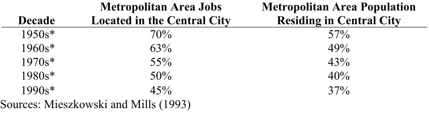
In the 1970s, 69 percent of the American population lived in what is classified as
metropolitan statistical areas (MSAs). In the 1980s that figure rose to 75 percent. By the 1990s,
77 percent of the nation’s population lived in a metropolitan area. Although a greater proportion
Table 2.1 Central City Population and Job Loss
Decade
Metropolitan Area Jobs Located in the Central City
Metropolitan Area Population Residing in Central City
1950s* 70% 57%
1960s* 63% 49%
1970s* 55% 43%
1980s* 50% 40%
1990s* 45% 37%
Sources: Mieszkowski and Mills (1993)
lives and works in the central city (Mieszkowski and Mills 1993). Table 2.1 demonstrates how
central cities in metropolitan areas lost percentages of both jobs and population over the decades.
It is clear from the figures in Table 2.1 that suburbanization has changed the American
landscape, bringing residents out of the center of metropolitan areas. This change in place of
residence and lifestyle in modern American society has led to a reliance on automobiles to access
jobs that are now located mostly in suburban areas throughout metropolitan regions. Even
though numerous jobs are now located in the suburbs where many people live and work,
automobiles are still necessary to access most employment locations due to the lack of adequate
public transportation in the suburbs. Therefore, today the automobile is not only a staple in the
lives of Americans, but a necessity, due to low-density development (Mieszkowski and Mills
1993). In fact, residential density is significantly related to the degree in which residents rely on
the automobile (Freeman 2001). Gone are the days of walking to and from places of daily
activities for many individuals.
The essential nature of this form of mobility allows jobs and homes to be miles apart. As
development continues outward from the central cities, housing and services grow farther apart.
This development pattern makes it just about impossible for pedestrian mobility. Therefore,
metropolitan areas. Additionally, the average time per trip is increasing, including the commute
to work, which society now accepts as commonplace (U.S. Department of Transportation 1999;
2004). It can be argued that sprawl is a direct result of a society centered on the automobile
(Glaeser and Kahn 2003).
It can be seen that sprawl has influenced community design, which in turn has created
environments that may significantly affect regular physical activity. In fact, some argue that
today’s built environment designs regular physical activity out of everyday life. Many times, the
quickest, if not only, way to get to places for normal daily activities, such as work, school, and
stores, is to drive. This dependence on automobiles has created communities where behaviors
beneficial to health, such as walking, are basically non-existent. Even more pervasive are
drive-through services, which allow individuals to bank, pick up dry cleaning, order food, and
ironically, get their medication, conveniently without ever taking a step. Even sidewalks are
designed “out” of many suburban areas making it impossible for individuals to safely walk from
place to place (MacLennan 2004).
Ewing, Pendall, and Chen (2002a) found that people living in sprawling areas tend to
drive more, own more cars, breathe more polluted air, face a greater risk of traffic fatalities, walk
less, and use public transit less than those who reside in areas that are not as sprawling. Such
factors lead people to weigh more and suffer from hypertension and other negative health
conditions. In contrast, those who reside in compact areas, such as New York City, tend to drive
less and walk more. These findings hold true even after controlling for sociodemographic
factors such as age, education, gender, and race. In fact, sprawl and its component factors
(dependence on automobiles, less physical activity, etc.) are found to be greater predictors of
The most likely way community design influences weight and health is by either
encouraging or discouraging routine physical activity in daily life. For most people, this means
walking to the store, to work, or other such places as a part of their daily routine. When it comes
to whether or not people get regular exercise in their leisure time, such as running, working out,
gardening, etc., the degree of sprawl seems to have very little influence, as people in both
sprawling and compact areas are equally likely to report they exercise in some fashion (McCann
and Ewing 2003). However, the degree of sprawl does make a difference in how people engage
in the most common, accessible, and free form of exercise – that of walking. Individuals in more
sprawling areas report less time walking in their leisure time than those who reside in compact
locales. For every 50-point increase in their sprawl scale, which ranges from 63.12 to 352.07,
McCann and Ewing (2003) find that people are likely to walk fourteen minutes less per month
for exercise, even when controlling for gender, age, education, ethnicity, and other factors. Their
study also shows that routine physical activity is a significant factor in lower BMI (Body Mass
Index) of individuals residing in more compact communities.
Do McCann and Ewing’s (2003) associations between urban form and physical activity
always hold true? What about a different side of this argument? Is it possible that those residing
in compact urban areas could walk less because they do not have as far to walk? Maybe they
take elevators more than those in sprawling areas because the buildings are tall, and taking
twenty or thirty flights of stairs is just not practical. On the other hand, those who reside in
sprawling areas may get more daily walking than those in dense areas because they have large
parking lots to traverse and sprawling buildings to walk around in instead of more compact, taller
Studies Looking at Sprawl and Health
There are a few studies that focus on measuring the health effects of sprawl, including
McCann and Ewing (2003), which is a follow-up study of research conducted by Ewing et al.
(2003). Both of these studies look at how sprawl affects physical activity, obesity, and chronic
disease, specifically diabetes, coronary heart disease, and hypertension. Their results show that
individuals in sprawling areas are more likely to have a higher BMI. McCann and Ewing found
that a 50-point increase in the degree of sprawl (a scale developed by Ewing et al. and measured
at the county level ranging from 63.12, indicative of more sprawl, to 352.07, indicative of a
compact area, with an average score of 100) relates to an increase in BMI by 0.17 points, which
translates to just over one pound for the average person. They also found that sprawl has a small
but significant effect on minutes walked per month and individuals in sprawling areas are more
likely to have hypertension. However, sprawl did not return any significant effects on diabetes
or coronary heart disease.
Another study also investigated the connection between sprawl and weight. Conducted
by Lopez (2004) and titled “Urban Sprawl and the Risk for Being Overweight or Obese,” an
association between levels of obesity in the South (20%) and urban sprawl is discussed. Lopez
contends that many of the metropolitan areas with the highest levels of urban sprawl are in the
southern United States. From this association, Lopez set forth to quantitatively test for statistical
significance between urban sprawl and the risk for being overweight or obese. Lopez’s analysis
shows that sprawl is associated with both an increased risk for being overweight (0.2% for each
1 point increase in his sprawl index, which is measured on a scale from 0 to 100, with 0 being the
sprawl index). He found the risk for being obese is greater than the risk for being merely
overweight when it comes to sprawl’s effect.
All three of these studies have some shortcomings though. One issue is the validity of
height and weight reported by participants (Lopez 2004; O’Toole 2002a; Bowlin et al. 1993;
Jackson et al. 1992). Critics such as O’Toole (2002a) point to the definition of BMI itself, which
is a standard measure of weight-to-height used to determine whether or not people are
overweight or obese, as being problematic because it does not distinguish between body types or
consider the overall health of an individual. There is also the issue of whether or not individuals
are being honest when reporting their height and weight.
Even though critics point to the fact that height and weight may be over- and understated,
respectively, in the BRFSS survey, it does not mean the data are completely flawed. Most
people will estimate their weight downward, providing a systematic error. As far as height, this
is more of a random error, since some people will provide a height that is too high and other will
provide a height that is too low. This is less problematic than the systematic error found with
weight. Every survey has its shortcomings and is plagued with the fact that some people will not
be honest (Rowland 1990). However, measures of BRFSS data have been determined to have
high reliability and validity, including height and weight (Nelson et al. 2001; Nelson et al. 2003).
Another issue with these studies is the fact that the data represent only one point in time
(Lopez 2004; O’Toole 2002a; Bowlin et al. 1993; Jackson et al. 1992). Hence, there is no way
of measuring whether or not respondents became overweight or obese while residing in the
metropolitan area in which they were surveyed. It may be the case that some became overweight
while residing in a very dense, less sprawling metropolitan area then moved to a very sprawling,
according to Lopez, most people tend not to change metropolitan areas; instead remaining in one
metropolitan area for long periods of time. Therefore, results should be a fairly appropriate
reflection of individuals’ exposure to sprawl. However, there is the issue of people making
intra-metropolitan moves, such as from the city center to a suburban area, or vice versa. In moves like
these, individuals are more likely to be exposed to varying degrees of sprawl.
This issue of varying degrees of sprawl leads to a final issue with Lopez’s (2004) study,
which is its significant ecological bias in that it does not reflect how sprawl varies within
metropolitan areas. Metropolitan areas are not homogenous, but rather differ from inner city to
suburbs, a factor not controlled for in Lopez’s study. Ewing et al. (2003) and McCann and
Ewing (2003) did, however, improve this issue that Lopez failed to address by employing a
sprawl index measured at the county level. This allows for a more precise measure of how
sprawl affects individual-level health without assuming that metropolitan-level sprawl is the
same within a region or affects individuals residing in very different parts of the same
metropolitan area in the same manner. A summary and critique of the different measures of
sprawl, along with additional ways of quantifying sprawl is discussed in detail in Chapter 4.
The urbanized environment has consequences for health, but exactly how does urban
sprawl relate to health outcomes? Is there a clear association? There may be many influences on
one’s health, and sprawl may only have a small and/or indirect effect. On the other hand, there
may be a strong association between sprawl and health outcomes. It is important now, more than
ever, to understand just how critical the decisions to plan, regulate, zone, and build the American
landscape are to individual-level health. The better the effects of these decisions are understood,
the better choices Americans can make in how to maintain their best health in the sprawling
CHAPTER 3
CONCEPTUAL FRAMEWORK
Many different ideas have emerged as to the origins of urban sprawl. Theories range
from anti-urban attitudes, racism, and increased affluence to economics and government policies.
The latter scenario theorizes that policies at the local, state, and national level, such as
homeowner subsidies, highway programs, infrastructure subsidies, and federal income tax
deductions, have fostered sprawl. These policies, according to proponents of this theory,
encourage city dwellers to move to the suburbs in favor of single-family home ownership instead
of apartment living in crowded, often dirty, cities. Such suburban home ownership was made
possible by government sponsorship of superhighways, suburban infrastructure, long-term
amortized mortgages, and federal mortgage insurance, so the theory goes (Bruegmann 2005;
Glaeser and Kahn 2003; Brueckner and Fansler 1983; Lindstrom and Bartling 2003).
Another theory favors that of technology as the cause of sprawl. As new communication
and transportation options were made available, growth was able to disperse from city centers.
According to this theory, in the past two centuries the railroad tended to concentrate growth and
population within cities. The automobile, however, made it possible to disperse this
concentration. This theory of sprawl advocates that before enhanced transportation options,
cities were dense, but this density yielded to highly dispersed growth with the introduction of the
automobile. This introduction of a personal means of long-range transportation, replacing
private horse-drawn carriages, made it possible for long-distance commutes to and from the
suburbs (Bruegmann 2005; Glaeser and Kahn 2003; Lindstrom and Bartling 2003).
complete blame on the highway system for the cause of sprawl. As ironic as it seems, these
roads were heavily supported by central-city interests. It was believed that a highway system
would reinforce the centrality of downtowns and make it easier for people from throughout the
region to get there, much like the railroads did in the past. Such roads did make getting
downtown much quicker, but they made it just as easy to leave the city as well. Even with such a
connection, there is no concrete evidence to prove that decentralization of cities and subsequent
sprawl throughout metropolitan areas was caused solely by postwar freeways. In fact, there is
the argument that the decentralization caused by the highway system was no different than the
decentralization caused by its predecessor, the railroad. Both have caused some dispersal, as
well as centralization. The amount of each depends on many factors, including individual
choices (Bruegmann 2005; Glaeser and Kahn 2003).
No matter how suburban or rural an area of a metropolitan region may be, most residents
are closely tied economically and socially to the urban world, and therefore are dependent on that
world (Bruegmann 2005; Glaeser and Kahn 2003; Lindstrom and Bartling 2003). This
dependence on the urban environment makes certain technologies, like automobiles and vast
road systems, necessary for mobility within metropolitan regions, many times at the expense of
pedestrian-friendly street networks. No matter what caused sprawl and continues to fuel it,
critics contend that it designs regular, beneficial, physical activity out of everyday life through
the patterns of mobility it promotes, which leads to a path model developed by Ewing et al.
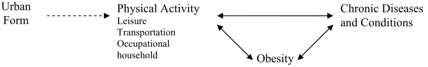
Figure 3.1 shows the model Ewing et al. (2003) developed from their analyses looking at
the relationships between sprawl, physical activity, obesity, and disease. They determined that
Figure 3.1 Established (Solid) and Speculative (Dashed) Relationships, from Ewing et al. (2003)
chronic diseases and conditions. Analyses also point to a speculative relationship between urban
form and physical activity. Ewing et all. (2003) developed their conceptual model (Figure 3.1)
after they performed their analyses of the data, but they did not conduct analyses to determine if
any indirect effects exist between the variables. One of my goals and contributions in this
dissertation research is to investigate possible indirect effects between sprawl, physical activity,
and body weight in regards to their relationship to health outcomes (depicted in Figure 3.2)
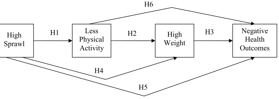
As it can be seen in my conceptual model (Figure 3.2), hypothesized relationships between the
variables depict direct and indirect effects. This conceptual model is the basis for my research. I
use it not only to look for associations between sprawl, physical activity, weight, and health
outcomes, but also text for indirect effects. I also look to answer questions, such as: 1) Is there a
significant association between sprawl and physical activity and if so, in what direction does
sprawl affect physical activity? Do individuals residing in less sprawling areas get significantly
more or less physical activity on average than those in more sprawling areas? and 2) Does
physical activity have a significant association with health outcomes by way of individual-level
weight? It is important to find out which, if any, associations between sprawl, physical activity,
weight, and health outcomes are the strongest in order to proceed with additional, more refined
research testing the causal relationships depicted in this model. Variables controlling for Chronic Diseases and Conditions Urban
Form
Physical Activity Leisure
Transportation Occupational
individual-level characteristics, such as sociodemographics, personal health, and region, are also
[image:31.612.84.538.151.312.2]included in statistical models in order to test each hypothesis.
Figure 3.2 Conceptual Model Used in this Dissertation
Hypotheses
Taking direction from previous studies and the conceptual model outlined above, I
hypothesize that there may be associations between sprawl, levels of physical activity, body
weight, and health outcomes. Therefore, I hypothesize the following:
Hypothesis 1 Sprawl is negatively related to physical activity. As sprawl increases, individual levels of physical activity decrease.
I suspect that built environmental form has a strong relationship to one’s health and that
the design of communities influences health by encouraging or discouraging routine physical
activity. Previous research suggests that people living in sprawling areas miss out on significant
health benefits available, such as walking to the store, to work, or other places as part of a daily
routine (McCann and Ewing 2003). This lack of beneficial regular physical activity may be
explained by over-reliance on automobiles and/or by patterns of streets within neighborhoods, Negative
Health Outcomes High
Sprawl
Less Physical Activity
High Weight H2
H1 H3
H6
H4
such as those found in many suburban subdivisions, as they seem to affect people’s propensity to
walk (Lopez 2004).
Hypothesis 2 Physical activity is negatively related to weight. As individual levels of physical activity decrease, individual weight increases.
Obesity has reached epidemic levels in the United States and physical inactivity is now
implicated as one of the causes of this condition. An increasing body of evidence suggests that
moderate forms of regular physical activity, such as walking, can have beneficial effects in
maintaining a healthy weight (McCann and Ewing 2003; Ewing et al. 2003). Unfortunately, the
majority of Americans report not obtaining enough exercise to meet the recommended weekly
minimum, and many Americans remain completely inactive during their leisure time (McCann
and Ewing 2003).
Hypothesis 3 Weight is positively related to negative health outcomes. As individual weight increases, so does the chance for individual-level negative health outcomes, such as diabetes, heart attack, heart disease, high cholesterol, hypertension, and stroke.
Health experts believe most Americans are overweight and conditions such as diabetes
and heart disease have reached epidemic levels as a consequence of such excessive weight
(McCann and Ewing 2003; Ewing et al. 2003). Such connections between body weight and
health conditions have long been documented, as well as an increase in the risk of mortality
coinciding with the severity of obesity (Calle et al. 1999).
Hypothesis 4 Sprawl is positively related to weight. As sprawl increases, so does individual-level weight.
This hypothesis seeks to determine if there is a direct effect between sprawl and weight.
determine how much variance in the individual-level variable of weight can be explained by the
macro-level variable of sprawl, controlling for other factors.
Hypothesis 5 Sprawl has a positive relationship to individual-level negative health outcomes. As sprawl increases, so does the chance for negative health outcomes, such as diabetes, heart attack, heart disease, high cholesterol, hypertension, and stroke, especially when mediated by physical activity and BMI.
Based on existing research, I hypothesize a positive zero-order correlation between
sprawl and negative health outcomes. As sprawl increases I expect a positive relationship
between sprawl and health problems to be revealed, especially when controlling for other
variables such as sociodemographics, personal health, and region. However, with the addition of
the mediating variables of physical activity and BMI, I hypothesize that the relationship between
sprawl and negative health outcomes will shrink and become statistically insignificant.
Hypothesis 6 Physical activity is negatively related to negative health outcomes. As individual levels of physical activity decrease, the chance for negative individual-level health outcomes, such as diabetes, heart attack, heart disease, high cholesterol, hypertension, and stroke increase.
Physical activity has been shown to have beneficial health outcomes (Perdue 2004;
McCann and Ewing 2003; Ewing et al. 2003; Ewing et al. 2002a); therefore, it is theoretically
logical to test for the variance explained by the relationship between these two individual-level
variables.
Additional Considerations
There are multiple additional variables besides sprawl, levels of physical activity, and
weight that need to be accounted for when statistically modeling for associations between sprawl
have termed this multi-variable association the ‘web of causation’ to refer to the fact that health
and disease are not explained by simple bivariate relationships (Krieger 1994). Instead, health
and disease are explained by a complex network of numerous interconnected risks and factors, or
multiple causations. Factors that may be important in explaining associations for health
outcomes have been absent in previous studies that examine sprawl and health outcomes at the
individual- and metropolitan-level. When looking at sprawl and health outcomes, other
mediating factors may be involved. Therefore, it is important to statistically model other
independent and control variables, such as race, age, gender, education, and region. In addition,
a variable that measures whether or not an individual is consciously increasing his or her level of
CHAPTER 4
MEASURES OF URBAN SPRAWL
Many different expressions have been used to describe urban sprawl. The uncontrolled,
unplanned spread of urban development into areas adjoining the edge of a city and a continuous
network of low density urban communities are just two descriptions of sprawl found in the
literature (Galster et al. 2001; Razin 1998). Complicating the situation of defining sprawl is the
fact that many times it is expressed as a noun, where it describes a condition characterizing all or
part of an urban area at a particular point in time. Other times it is used as a verb, describing the
process of converting land over a period of time from non-urban to urban uses, or as changes in
the extent or intensity of urbanization, particularly at urban fringes. By defining sprawl as either
a condition (a noun) or a process (a verb), ambiguity and idiosyncrasy set in, making it
impossible to know with confidence the causes, consequences, or effects of sprawl, as well as the
effectiveness of policies designed to control it (Wolman et al. 2005; Galster et al. 2001; Fulton et
al. 2001; Ewing et al. 2002a). Ambiguity in defining sprawl creates problems regarding its
measurement.
Measures of sprawl vary as much as the definitions for sprawl itself and range from the
simple to the complex. Such varied ways of measurement make it difficult to pinpoint what
exactly is meant by sprawl, how it should be measured, and the geographical areas and types of
land that should be considered (Wolman et al. 2005). In order to track sprawl, scholars, as well
as planners and policy makers, need a way to define and measure it, as well as be able to
demonstrate how and to what degree sprawl has genuine implications (Wolman et al. 2005;
components of sprawl are found throughout the literature, and several recent studies address how
to define and empirically operationalize the concept.
This section discusses recent studies that focus on sprawl and health and describe their
measures of sprawl. It concludes with a discussion of the measure of sprawl in which I use for
analyzing my conceptual model.
Studies Focusing on Sprawl and Health Outcomes
There are two recent studies focusing on sprawl and its association with health. In a
study looking at the measurement, distribution, and trends of sprawl in the 1990s, Lopez and
Hynes (2003) define sprawl as a process where the overall pattern of metropolitan land
development consists of populations residing in lower-density developments. In Lopez and
Hynes’ sprawl index, metropolitan areas with much of their population concentrated in certain
areas are considered less sprawling than metropolitan areas with a population that is evenly
distributed across the entire region. Even though their sprawl index is fairly simple, it is a useful
measure of sprawl and is based on accessible public data. Lopez and Hynes contend that
concentration (the distribution of density) is an important factor in measuring sprawl and state
that focusing on density computations alone across metropolitan areas will result in an index that
is misleading, because sprawl is also a function of how density is distributed. Unfortunately
Lopez and Hynes’ scale fails to reflect the spatial positions of low- and high-density tracts.
Additionally, their sprawl index is based on subjective cut-off points for low- and high- density
tracts. If their cut-off points were changed, so would their sprawl index calculations (Jaret et al.
in his study looking at the relationship between sprawl and the risk for being overweight or
obese.
Another important study of sprawl that measured and computed it for U. S. metropolitan
areas was done by Ewing et al. (2002a, b). This was a landmark study conducted by Rutgers and
Cornell Universities for Smart Growth America, a national public interest group that promotes
smart growth policies. In this study, the researchers define sprawl as a process where
development across the landscape far outpaces population growth and provides people with poor
accessibility. Ewing et al. assert that a sprawling landscape consists of: (1) a population that is
dispersed in extensive low-density development; (2) homes, shops, and workplaces that are
rigidly separated from one another; (3) a network of roads that consist of large blocks with poor
access; and (4) a lack of well-defined activity centers, such as downtowns. These authors state
that other features of sprawl, such as the lack of transportation choices and difficulty walking,
are results of these four unique dimensions of sprawl.
Ewing et al. set forth to create a sprawl index that can be measured and analyzed based
on the four dimensions of sprawl they identify. Each dimension comprises several measurable
components that were tested to ensure they added a unique perspective to the overall
representation of sprawl. For example, residential density includes the proportion of residents
living in very spread-out areas, the proportion of residents living close together, and overall
density, as well as other measures. Ewing et al. argue that they have created the most
comprehensive attempt to define and quantify sprawl in the United States. A list of the four
factors measuring sprawl and the sources for data can be found in their study.
Ewing et al. (2002a, b) computed their four dimensions of sprawl by performing factor
the factor loadings, they created an index score for each dimension, as well as a fifth composite
score, for 83 metropolitan areas. Their resulting indices are one of the most comprehensive
attempts to define and quantify sprawl in the United States. However, their scores are based on
1990 Census data, as there was little data available for the year 2000 when they created their
index. Therefore, their index is not as up to date as other sprawl indices and leaves researchers
who desire to use the Ewing et al.’s sprawl method the task of computing their own, more up to
date index. Since metropolitan areas are dynamic and increase in size and area over time, it is
imperative that the most up-to-date index on sprawl be utilized for any type of analysis and/or
comparison (Jaret et al. 2009).
Another study that focuses on sprawl and health was conducted by McCann and Ewing
(2003), which was derived from the landmark study by Ewing et al. (2003). The McCann and
Ewing research was a follow up study utilizing a county-level sprawl index developed for the
Ewing et al. research. In addition to their metropolitan-level sprawl index, Ewing et al. also
developed a county-level sprawl index, using a very similar measure to their metropolitan-level
index. While looking at measuring the health effects of sprawl as it relates to physical activity,
obesity and chronic disease, McCann and Ewing contend that although the metropolitan-level
sprawl index developed by Ewing et al. is an extremely comprehensive means of measuring
sprawl, they needed a finer degree of information for their study. So, they turned to the
county-level sprawl index developed by Ewing et al. This research conducted by McCann and Ewing is
very similar to my dissertation. The main differences are the fact that I also test for indirect
effects among the variables and employ additional health outcomes.
Ewing et al.’s (2003) county-level sprawl index used relevant data from the Ewing et al.
variables from the U.S. Census and the Department of Agriculture’s Natural Resources Inventory
measure on residential density and street network connectivity. Ewing et al. conducted factor
analysis to derive their sprawl index from their data sources. Even though fewer data are
available at the county level and their index is less comprehensive than the metropolitan-level
sprawl index, it is still the most complete measurement of sprawl available at the county level.
Ewing et al. (2003) developed their county-level sprawl index based on variables that
reflect two dimensions of sprawl – residential density and street network connectivity, two of the
original four dimensions employed by Ewing et al. (2002a, b). Overall, they utilized six
variables to develop their sprawl index, which include: (1) population density per square mile;
(2) percentage of population living at densities less than 1,500 per square mile; (3) percentage of
population living at densities greater than 12,500 per square mile; (4) net population density of
urban lands (excludes lands not directly related to the figure, such as green spaces and roads); (5)
average block size in square miles; and (6) percentage of small blocks (≤ 0.01 square mile). The
technique utilized by Ewing et al. provided the researchers with a sprawl index that is a
comprehensive measurement of sprawl at a finer, more appropriate level. A list of the factors,
variables, and sources Ewing et al. utilized for their county-level sprawl index is listed in
Appendix B.
The sprawl index that Ewing et al. (2003) developed is somewhat counterintuitive in that
high scores indicate low levels of sprawl, whereas low scores represent high levels of sprawl.
For their county-level sprawl index, scores range from 63.12 (high sprawl) for Geauga County
(which is a mostly rural county) in the Cleveland, OH metropolitan area to 352.07 (low sprawl)
for the very compact New York County (Manhattan) in the New York, NY metropolitan area.
score of 100. It should be mentioned that counties on the lower end of the scale (those indicative
of high sprawl by this county-level index) are actually more exurban than suburban and therefore
do not necessarily accurately represent sprawl for certain counties, like that of for Geauga
County, OH.
Conclusion
When determining an appropriate method for quantifying sprawl, it is important to keep
in mind that sprawl is very subjective in nature. It is also imperative to capture as many vital
aspects of sprawl as possible, as well as to determine the correct geographical area and level at
which to calculate it. Variables that accurately represent the theoretical abstraction of sprawl
must be considered in order to objectively measure it. Since operational variables are seldom
complete and accurate representations of underlying constructs and they are subject to
measurement and sampling errors, it is important to use multiple variables in order to capture the
essence of the construct. One or two variables cannot adequately capture and truly represent the
inherent complexity of sprawl. Therefore, multiple variables are needed to represent its various
dimensions (Ewing et al. 2002a). Unfortunately, many studies fall short in determining the vital
aspects of sprawl and measuring it adequately.
Keeping in mind that sprawl is a construct that must be operationalized properly, I utilize
the Ewing et al. (2003) county-level sprawl index due to its multiple-variable representations of
two dimensions of sprawl. The Ewing et al. county-level sprawl index is an excellent choice for
my research because spatial form is inherently multidimensional and does not stem from one
single process. Rather, it is a complex phenomenon that interconnects many different social and
economic processes (Timms 1971; Massey and Denton 1988). Even though no absolute
Ewing et al. (2002a. b. 2003) and McCann and Ewing (2003). For this reason, I utilize the
Ewing et al. index (the same one utilized in the McCann and Ewing study) for my research
concerning the connection between sprawl, physical activity, weight, and health outcomes.
Since certain data were not available for all counties, Ewing et al. (2003) lost a total of 73
counties that were included in their metropolitan-level sprawl index. However, they gained 90
additional counties by incorporating other metropolitan areas, such as Chattanooga, TN-GA,
Mobile, AL, and Augusta-Aiken, GA-SC in their study. Additionally, the BRFSS does not
report data for certain counties that are included in the Ewing et al. (2003) sprawl index;
therefore, I lose a certain amount of cases from the BRFSS dataset because they do not have a
corresponding county-level sprawl index.
I also have the issue with more rural and/or exurban counties like Geauga, OH. I have
kept counties that are more rural or exurban in my analyses for several reasons. Counties like
Geauga, OH are metropolitan counties, as defined by the U.S. Census Bureau, for a reason.
They are tied to their respective metropolitan core both socially and economically and are not
recent additions to metropolitan areas. They have been a metropolitan county for at least ten
years. Additionally, exurbanites often have to travel farther than their suburban counterparts to
get to places such as stores, schools, etc. because commercial development is often farther apart
in the exurbs.
Sprawl index scores for all 448 counties included in the Ewing et al. (2003) and McCann
CHAPTER 5
METHODOLOGY
Most of the data for analyzing my conceptual model comes from the Behavioral Risk
Factor Surveillance System’s (BRFSS) 2003 Chronic Disease and the Environment dataset
(Centers for Disease Control and Prevention 2003). The BRFSS is an annual telephone survey
of adults that includes more than two hundred self-reported and calculated variables. It is an
excellent source of information concerning the health status and habits for the U.S. population.
This is the same source for data in the Ewing et al. (2003) and McCann and Ewing (2003)
research. Instead of 2003 data, those studies incorporated data from the years 1998 to 2000.
The Behavioral Risk Factor Surveillance System is an annual telephone survey that
utilizes a questionnaire distributed to each of the 50 states. It is developed jointly by the CDC’s
Behavioral Surveillance Branch (BSB) and the States. The questionnaire is constructed at the
BRFSS Working Group annual meeting in February of each year. Representatives from the
National Center for Chronic Disease Prevention and Health Promotion (NCCDPHP) and other
parts of the CDC propose BRFSS questions for consideration, along with input and feedback
each state provides on the proposed content. After their annual meeting the BSB designs the
core components, as well as optional modules, and sends them to the states, where each state
may add questions they have designed or acquired for their own purposes for health surveillance.
After the questionnaire has been designed and distributed to each of the 50 states, the
BSB provides each state samples of telephone numbers. Each state must then review its
sampling methodology with a state statistician and BSB to make sure data collection procedures
are in place and that they follow correct methodology. States then conduct interviews each
interviewing (CATI) computer file, then edit and correct completed interviews. States then
submit their data to the BSB where it is weighted according to state-specific population estimates
and distributes the information accordingly.
The BRFSS survey protocol requires all states to ask the core component of questions
without modification; although states may choose to add any of the optional modules, as well as
state-added questions after the core component. Electronic monitoring is a routine and integral
part of the monthly survey procedures for all interviewers. If electronic monitoring is not used,
then a 5% random sample of each month’s interviewees must be called back to verify the quality
of selected responses.
The BSB states that an eligible household for surveying is a housing unit that has a
separate entrance where occupants eat separately from other persons on the same property and
such household is occupied by its members as a principal or secondary place of residence.
Eligible household members include those who are 18 years and older, related or unrelated,
roommates, and domestic workers who consider the dwelling their home. Completed interviews
must include age, race, and gender. If such values are not entered, imputed values are generated
and used only to assign post-stratification weights. The average time to complete an interview
for the 2003 BRFSS annual survey was 20.8 minutes and the response rate (defined as completed
interviews plus partially completed interviews, divided by all eligible interviews) was 48.3%
(Centers for Disease Control and Prevention 2003).
It should be noted that not all cases included in the 2003 BRFSS dataset were utilized due
to reconciliation with Ewing et al.’s (2003) sprawl index. After reconciliation, I lost 115
counties from their sprawl index because they were not included in the BRFSS dataset.
Ewing et al. sprawl index. However, after reconciliation between the Ewing et al. county-level
sprawl index and the 2003 BRFSS dataset, there were cases from 326 counties across 109
metropolitan areas in 40 states included in analyses. Every effort was made to ensure the BRFSS
dataset was reconciled with the Ewing et al. sprawl index accurately. This was done by
matching each case in the BRFSS individual-level database with its correct county-level sprawl
index score. Matching was completed using the FIPS code, a code employed by the U.S.
government to assign each county in the nation a unique number. The BRFSS includes these
codes and lists them for each case. By looking up the FIPS code for each county in Ewing et
al.’s sprawl index, I was able to match each case with its correct sprawl index score.
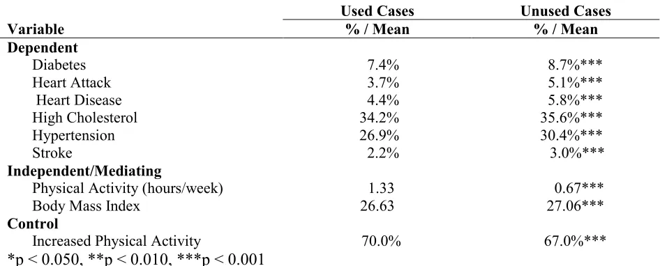
Since I was unable to use certain cases from the BRFSS dataset in analyses, I compared
the means of certain variables to determine if cases used in analyses differ systematically from
the cases not used. Table 5.1 shows the results of this comparison. It details the difference in
means between used and unused cases. T-tests return highly significant results stating that
[image:44.612.67.540.486.677.2]unused cases do in fact differ systematically from those that were used in analyses.
Table 5.1 Difference in Means Significance Testing
Used Cases Unused Cases
Variable % / Mean % / Mean
Dependent
Diabetes 7.4% 8.7%***
Heart Attack 3.7% 5.1%***
Heart Disease 4.4% 5.8%***
High Cholesterol 34.2% 35.6%***
Hypertension 26.9% 30.4%***
Stroke 2.2% 3.0%***
Independent/Mediating
Physical Activity (hours/week) 1.33 0.67***
Body Mass Index 26.63 27.06***
Control
Increased Physical Activity 70.0% 67.0%***
In order to better understand the data and variables in this study, dependent, independent,
and control variables are discussed below. Table 5.2 lists descriptive statistics for all variables
included in analyses.
Dependent Variables
There are six different dependent variables. They include diabetes, heart attack, heart
disease, high cholesterol, hypertension, and stroke. All data for the dependent variables were
obtained from the BRFSS dataset.
Diabetes. This variable shows whether or not individuals in the sample have diabetes. It
is operationalized as being either yes, no, or yes – pregnancy-related diabetes. I coded all cases
that were yes – pregnancy related diabetes, which was 0.90% of the sample, as no because it is a
temporary condition related to some pregnancies and is not a normal day-to-day condition as
with other chronic cases of diabetes. In my final dataset, 7.4% of the sample has diabetes.
Heart Attack. This variable shows whether or not individuals in the sample have ever
had a heart attack. In my final dataset, 3.7% of individuals in the sample have had a heart attack.
Heart attack was not defined in the survey; rather interviewers relied on whether or not
interviewees were ever told by a medical professional that they have had a heart attack.
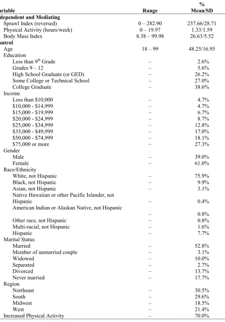
Table 5.2 Descriptive Statistics
Variable Range
% Mean/SD Dependent
Diabetes – 7.4%
Heart Attack – 3.7%
Heart Disease – 4.4%
High Cholesterol – 34.2%
Hypertension 26.9%
Table 5.2 continued
Variable Range
% Mean/SD Independent and Mediating
Sprawl Index (reversed) 0 – 282.90 237.66/28.71
Physical Activity (hours/week) 0 – 19.97 1.33/1.59
Body Mass Index 8.38 – 99.98 26.63/5.52
Control
Age 18 – 99 48.25/16.95
Education
Less than 9th Grade – 2.6%
Grades 9 – 12 – 5.6%
High School Graduate (or GED) – 26.2%
Some College or Technical School – 27.0%
College Graduate – 38.6%
Income
Less than $10,000 – 4.7%
$10,000 - $14,999 – 4.7%
$15,000 - $19,999 – 6.7%
$20,000 - $24,999 – 8.7%
$25,000 - $34,999 – 12.8%
$35,000 - $49,999 – 17.0%
$50,000 - $74,999 – 18.1%
$75,000 or more – 27.3%
Gender
Male – 39.0%
Female – 61.0%
Race/Ethnicity
White, not Hispanic – 75.9%
Black, not Hispanic – 9.9%
Asian, not Hispanic – 3.1%
Native Hawaiian or other Pacific Islander, not
Hispanic – 0.4%
American Indian or Alaskan Native, not Hispanic
– 0.8%
Other race, not Hispanic – 0.8%
Multi-racial, not Hispanic – 1.6%
Hispanic – 7.7%
Marital Status
Married – 52.8%
Member of unmarried couple – 3.1%
Widowed – 10.0%
Separated – 2.7%
Divorced – 13.7%
Never married – 17.7%
Region
Northeast – 30.5%
South – 29.6%
Midwest – 18.5%