https://doi.org/10.5194/hess-22-6505-2018 © Author(s) 2018. This work is distributed under the Creative Commons Attribution 4.0 License.
Temporal- and spatial-scale and positional effects on rain erosivity
derived from point-scale and contiguous rain data
Franziska K. Fischer1,2,3, Tanja Winterrath4, and Karl Auerswald1
1Lehrstuhl für Grünlandlehre, Technische Universität München, 85354 Freising, Germany 2Bayerische Landesanstalt für Landwirtschaft, 85354 Freising, Germany
3Außenstelle Weihenstephan, Deutscher Wetterdienst, 85354 Freising, Germany 4Zentrale, Deutscher Wetterdienst, 63067 Offenbach am Main, Germany
Correspondence:Karl Auerswald ([email protected]) Received: 1 June 2018 – Discussion started: 18 June 2018
Revised: 13 November 2018 – Accepted: 18 November 2018 – Published: 14 December 2018
Abstract.Up until now, erosivity required for soil loss pre-dictions has been mainly estimated from rain gauge data at point scale and then spatially interpolated to erosivity maps. Contiguous rain data from weather radar measure-ments, satellites, cellular communication networks and other sources are now available, but they differ in measurement method and temporal and spatial scale from data at point scale. We determined how the intensity threshold of erosive rains has to be modified and which scaling factors have to be applied to account for the differences in method and scales. Furthermore, a positional effect quantifies heterogeneity of erosivity within 1 km2, which presently is the highest resolu-tion of freely available gauge-adjusted radar rain data. These effects were analysed using several large data sets with a to-tal of approximately 2×10⁶erosive events (e.g. records of 115 rain gauges for 16 years distributed across Germany and radar rain data for the same locations and events). With de-creasing temporal resolution, peak intensities decreased and the intensity threshold was met less often. This became espe-cially pronounced when time increments became larger than 30 min. With decreasing spatial resolution, intensity peaks were also reduced because additionally large areas without erosive rain were included within one pixel. This was due to the steep spatial gradients in erosivity. Erosivity of single events could be zero or more than twice the mean annual sum within a distance of less than 1 km. We conclude that the re-sulting large positional effect requires use of contiguous rain data, even over distances of less than 1 km, but at the same time contiguously measured radar data cannot be resolved to point scale. The temporal scale is easier to consider, but with
time increments larger than 30 min the loss of information increases considerably. We provide functions to account for temporal scale (from 1 to 120 min) and spatial scale (from rain gauge to pixels of 18 km width) that can be applied to rain gauge data of low temporal resolution and to contiguous rain data.
1 Introduction
Prediction of rain-induced soil erosion using models like the Universal Soil Loss Equation (USLE) requires quantification of the potential of rain to cause soil detachment and trans-port. This potential is called rainfall erosivity and is typically obtained from point rainfall measurements using rain gauges. For the conversion of erosivities from point to spatial infor-mation, isolines, interpolation techniques and relations to pa-rameters such as the mean summer rainfall depth have been used (Rogler and Schwertmann, 1981; Wischmeier, 1959; Wischmeier and Smith, 1958, 1978). The characteristic re-lation between erosivity and rain depth of the same period was termed erosivity density and used in RUSLE2 (Dabney et al., 2012; USDA, 2013). It is recommended for areas with poor data availability (Nearing et al., 2017).
Fair-man et al., 2015), 2×2 km2(Koistinen and Michelson, 2002; Michelson et al., 2010) or 4×4 km2(Hardegree et al., 2008). Contiguous data of even coarser scale may result from other sources such as satellite data (Vrieling et al., 2010, 2014) or the output of regional climate models (e.g. Christensen et al., 2007; Flato et al., 2013).
Despite the important advantage that radar rain data are contiguous and temporally resolved, they cannot easily be used in place of rain gauge data for erosivity estimations because the scales of measurement differ a lot between both techniques. While rain gauges measure the rain near ground level at point scale (in Germany the collection area is 200 cm2), radars usually deliver rain measurements with an azimuthal resolution of approx. 1◦and a range of 125 to 1000 m. The data are then typically aggregated in grids of square pixels 1 to 16 km2in size. Rain intensity may differ greatly between point and grid measurements due to reduc-tion in peak intensities with decreasing temporal and spa-tial resolution. Furthermore, sources of error differ between both measurement techniques. For radar measurements, er-rors may result from shading of rain cells by objects such as buildings, orographic elevations or hydrometeors and from the influence of the melting layer causing bright-band effects (Wagner et al., 2012). Major limitations of rain gauges are caused by adhesion, evaporation, wind drift and splashing (Habib et al., 2001). Finally, strong gradients can, in par-ticular, be expected for thunderstorm cells of limited spa-tial extent. Thus, heterogeneity within pixels will be espe-cially pronounced for erosive rains (Fiener and Auerswald, 2009; Fischer et al., 2016; Krajewski et al., 2003; Pedersen et al., 2010; Peleg et al., 2016). This heterogeneity cannot be resolved but needs to be quantified because it is the un-certainty that can be expected for predictions at a resolution higher than the pixel size. This uncertainty also applies in cases where a point measurement of rain erosivity is within a certain distance (e.g. 1 km) from the target area for which erosion is to be calculated. The resulting deviation between point measurement and grid pixel average will be called “po-sitional effect” in the following. The po“po-sitional effect also de-termines the uncertainty, caused by the spatial variability of rain, of soil loss predications in the proximity of a point rain measuring location. This positional effect should level out in long-term measurements as long as grid pixels are small enough not to include a consistent orographic pattern.
By definition in the USLE, erosivity is the product of a rain event’s maximum 30 min intensity and its total kinetic energy (Wischmeier and Smith, 1958). Both factors depend on rain intensity; thus, intensity is squared in erosivity. Con-sequently, a difference in rain intensity of just 10 % would result in difference in erosivity of 21 %. Therefore, larger ef-fects of variation in rain intensity can be expected for erosiv-ity than for rainfall. In particular, an average of squares, as obtained from several point measurements within an area of non-uniform rainfall, will always be higher than the square of the average calculated from the same measurements. This
difference between both squares caused by the difference in spatial scale of the measurements is expected to be a robust factor in the long run. We will call this the “spatial-scale ef-fect”. A spatial-scale effect for erosivity, to the best of our knowledge, has not been studied. This is probably due to the novelty of operational radar measurements and the lack of long-term data sets required for erosivity estimations. Long-term and revised radar rain data now exist and can help to im-prove contiguous erosivity and soil loss estimations. There-fore, it is crucial to know to what extent erosivity, and sub-sequently also soil loss, is underestimated due to the spatial-scale effect by gridded rain data as provided by radar mea-surements and also by climate models or satellites that em-ploy an even coarser spatial resolution than typical radars (Chen and Knutson, 2008; Vrieling et al., 2014). Rain inten-sities from radar may additionally be smoothed by measur-ing and subsequent processmeasur-ing procedures. The contribution of erosivity underestimation due to these procedures is called the “method effect” in the following. Thus, the difference in erosivity from rain gauge data and from radar data is caused by spatial-scale and method effects.
Another effect is induced by the temporal scale of the data used for erosivity calculations. With decreasing tempo-ral resolution, maximum 30 min intensity and hence erosivity are increasingly underestimated. Therefore, temporal scaling factors are required to compensate for this underestimation (e.g. Auerswald et al., 2015; Agnese et al., 2006; Istok et al., 1986; Williams and Sheridan, 1991; Weiss, 1964; Yin et al., 2007). These are especially important for contiguous data, for which temporal resolution of rain data is decreased, often to 60 min, as a requirement for the adjustment to rain gauge data and to reduce the enormous amount of data caused by the high spatial resolution and wide spatial and temporal cov-erage.
We therefore hypothesize that (1) with decreasing tempo-ral and spatial resolution of rain data, calculated erosivities decrease due to a smoothing of intensities; (2) radar mea-surements cause an additional underestimation of erosivities due to the measuring principle and the required calculation and correction steps; and (3) large uncertainty of erosivity within 1 km2 is due to strong gradients of erosive rains as determined by the positional effect. The effects of hypothe-ses (1) and (2) have to be compensated for by changes in the calculation of erosivity, while the effect of hypothesis (3) quantifies uncertainty of erosivity of individual events at any location within an area of 1 km2around a rain gauge. We will quantify these effects and discuss their implications.
2 Material and methods 2.1 Data sets
(for an overview see Table 1). The spatial resolution from point scale to 1 km pixel width (with an intermediate pixel width of 0.5 km) was covered by a high-density network of 12 rain gauges which operated over 4 years within an area of 1 km2 (taken from Fiener and Auerswald, 2009; for lo-cation of the measuring site see Fig. 1a; for the spatial dis-tribution of rain gauges see Fig. 1c). The data of the net-work comprised 542 events at point scale. The spatially in-tegrated hyetographs at 0.5 or 1 km pixel width generated by the Thiessen polygon method (see Fig. 1c) will be referred to as “pseudo-radar” data.
Point scale and 1 km pixel width were also compared for a much wider data set covering 16 years and the whole of Germany. Erosivities at 115 rain gauges were compared to erosivities obtained from radar data with 1 km resolution (for location of the rain gauges and the coverage of weather radars see Fig. 1a). Rain gauge data were taken from the Cli-mate Data Center of the German Weather Service (Deutscher Wetterdienst: DWD; ftp://ftp-cdc.dwd.de/pub/CDC/, last ac-cess: 11 December 2018). DWD also provided the radar data, which were a revised version of the RADar OnLine ANeichung (RADOLAN) radar rain data product (Winter-rath et al., 2012, 2017). This resulted in point–pixel pairs for
>20 000 erosive rain events. For this data set the effect of temporal resolution was also evaluated. For spatial resolu-tions lower than 1 km pixel width (up to 18 km pixel width), a third data set was used. It comprised 1.9×10⁶ events at 1 km pixel width determined by radar measurements within an area of 800×600 km2(Table 1).
Precipitation measurements of the DWD station network were conducted with OTT Pluvio weighing rain gauges (OTT Hydromet GmbH, Kempten, Germany) with a collec-tor area of 200 cm2, a measurement range of 0–1800 mm h−1 and a 1 min resolution of 0.1 mm h−1. The precipitation data passed a quality control system testing for complete-ness, carrying out climatological tests, and checking con-sistency over time as well as internal and spatial consis-tency (Spengler, 2002; Kaspar, 2013). The data were nei-ther corrected for wind drift effects nor homogenized. A thorough overview of the precision of rain gauge mea-surements is given in Vuerich et al. (2009). Information on the stations’ metadata can be found in the Climate Data Center (ftp://ftp-cdc.dwd.de/pub/CDC/observations_ germany/climate/hourly/precipitation/historical/; last access: 11 December 2018) of DWD.
The DWD weather radar network underwent several up-grades during the analysis period. In the beginning of the considered time period five single-polarization systems (DWSR-88C, AeroBase Group Inc., Manassas, USA) op-erated without a Doppler filter, the latter being added be-tween 2001 and 2004. Bebe-tween 2009 and today, DWD has exchanged the network of C-band single-polarization sys-tems of the next generation of type METEOR 360 AC (Gematronik, Neuss, Germany) and DWSR-2501 (Enterprise Electronics Corporation, Enterprise, USA) by modern
dual-polarization C-band systems of type DWSR-5001C/SDP-CE (Enterprise Electronics Corporation), all equipped with a Doppler filter. During the time of exchange, a portable in-terim radar system of type DWSR-5001C was installed at some of the sites. Radar data underwent an operational qual-ity control system. They were adjusted to gauge data within a reprocessing suite applying a consistent software version (version 2017.002) and optimized quality control algorithms with 5 min resolution (Winterrath et al., 2018a) and 60 min resolution (Winterrath et al., 2018b).
2.2 Erosivity calculation procedures
Following Wischmeier (1959) and Wischmeier and Smith (1978) erosivity of a single rain event (Re) was
calcu-lated as the product of the maximum 30 min rain intensity (Imax30) and the kinetic energy (Ekin) (Eq. 1). A rain event
is erosive by definition if it has a total precipitation (P )
of at least 12.7 mm or a minimum Imax30 of 12.7 mm h−1
(min(Imax30)).
Re=Imax30·Ekin (1)
TheEkin,i per millimetre rain depth (in kJ m−2mm−1) was calculated for intervalsiof constant rain intensityI follow-ing Eq. (2a)–(2c). For all intervalsi,Ekin,iwas multiplied by the rain amount of this interval and then summed up to yield
Ekinfor the entire event.
Ekin,i= 11.89+8.73×log10I
×10−3
for 0.05 mm h−1≤I <76.2 mm h−1 (2a)
Ekin,i=0 forI <0.05 mm h−1 (2b)
Ekin,i=28.33×10⁻³ forI ≥76.2 mm h−1 (2c) When Imax30 was derived from data with intervals longer
than 30 min,Imax30was determined as the maximum rain
in-tensity of the event. Erosive events are separated from each other by rain breaks of at least 6 h (Wischmeier and Smith, 1958, 1978). For example, using 60 min rain data, we defined events as being separate when five subsequent 60 min inter-vals without rain occurred. This assumes that rain events stop and start on average in the middle of the first and the last non-zero rain interval. The same concept was used for all data sets with temporal resolutions>60 min.
The annual erosivity of a specific year (Ry) is the sum of
Re of all n erosive events within this year. The long-term
average annual erosivity (R) is then calculated as
R=1
k
Xk j(
Xn
iRe,i)j= 1
k
Xk
jRy,j, (3) which is the average ofRyfor a number ofk years, in the
case of this study 16 years.
Figure 1. (a)Locations of the 115 rain gauges (dots), the coverage (circles) of the 17 weather radars (crosses) and the location of the 12 rain gauges used for the pseudo-radar data (square; size exaggerated) in Germany.(b)One rain gauge (dot) within one 1×1 km2pixel (bounding box) and isolines of rain depth (taken from Fiener and Auerswald, 2009) illustrating the variability of a single erosive rain event at 1×1 km2grid scale causing positional effects.(c)Distribution of the 12 rain gauges (dots) within an area of 1×1 km2(bounding box) and their corresponding Thiessen polygons. Dashed lines separate the area to a spatial scale of 0.5×0.5 km2.
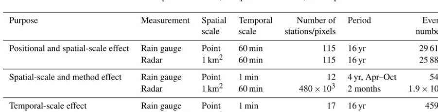
Table 1.Overview of the data used to determine the positional effect, the spatial-scale effect, the temporal-scale effect and the method effect.
Purpose Measurement Spatial Temporal Number of Period Event
scale scale stations/pixels number
Positional and spatial-scale effect Rain gauge Point 60 min 115 16 yr 29 610
Radar 1 km2 60 min 115 16 yr 25 884
Spatial-scale and method effect Rain gauge Point 1 min 12 4 yr, Apr–Oct 542
Radar 1 km2 60 min 480×103 2 months 1.9×10⁶
Temporal-scale effect Rain gauge Point 1 min 17 16 yr 4599
Radar 1 km2 5 min 17 16 yr 3924
is the unit most often used in Europe and because of its sim-plicity. The units can be easily converted by multiplying the values in N h−1by a factor of 10 to yield MJ mm ha−1h−1.
2.3 Determination of scale effects
The smoothing caused by decreasing resolution in time and space mainly decreases intensity, while the total amount of rainfall should, in principle, be unaffected. This decrease in intensity has two consequences. First, the intensity threshold
min(Imax30) that defines an erosive event is less often met and
[image:4.612.73.524.461.576.2]tempo-ral scales. It is caused by the additional smoothing resulting from the radar technique and the adjustment and correction steps subsequently required. It may also include the errors of rain measurement that differ between the rain gauge and radar methods. The positional effectpRe describes the aver-age relative deviation of erosivity of single events derived at 1 km resolution and at point scale from rain gauges located within the respective 1 km pixel including the spatial-scale and method effects. The positional effect cannot be used for correction, but it is a measure of variability within a certain pixel.
Adjusting the intensity threshold to account for smoothing at low resolution is appropriate only for the temporal reso-lution. With decreasing spatial resolution some areas will be included within a pixel that actually received erosive rain, while other areas within the pixel did not. Without adjust-ment of the intensity threshold the entire pixel may be classi-fied as non-erosive, while adjustment of the threshold would then indicate an erosive event also in those areas within a pixel where no erosive rain had occurred. Adjusting the in-tensity threshold with decreasing spatial resolution could not correct both errors simultaneously. Even more important, the criterion of breaks that separate between events is biased for large areas. Any rain at some place within a large pixel ab-rogates an existing break even if it does not fall at a site that experienced an erosive rain event. The loss of a break with in-creasing pixel size decreases the number of events even when all events are considered. Adjusting the number of events in this case would be a wrong correction. Hence for the spatial resolution the threshold effect was included insσ, while for the temporal-scale effect the intensity threshold could be ad-justed. As a result the number of erosive events can correctly be estimated at low temporal resolution with this adjustment at point scale, while for a spatial resolution lower than point scale the number of erosive events will be wrong compared to point scale. Only the sum of erosivities over a longer pe-riod of time (months, years or longer) can then be corrected with the spatial scaling factor.
The hyetographs of the high-density network of 12 rain gauges were spatially integrated to yield hyetographs at 0.5 or 1 km pixel width. The average deviation of annual ero-sivities calculated from hyetographs at point scale and from spatially integrated hyetographs at 0.5 or 1 km pixel width yielded the spatial scaling factorssσ=0.5andsσ=1. The
indi-vidual deviation of event erosivities at point scale from the average was due to the positional effectpRe(for an example see Fig. 1b). The average positional effectpRewas calculated as the geometric mean of thekratios ofRederived from rain
gauge (σ =0) and 1 km2 pixel data (σ=1), for which nei-ther rain gaugeRenor pixelRewas zero:
pRe=10 (Pk
i=1log10(Re,σ=0/Re,σ=1)i/ k). (4) The positional effects were determined separately for events withRe,σ=1larger andRe,σ=1lower thanRe,σ=0. Rains that
were erosive at only one of both spatial scales were excluded from the calculation of the geometric mean, and the percent-ages of these events were determined for both cases.
Erosivity at point scale and at 1 km2 pixel scale were also compared based on>20 000 erosive rain events at 115 lo-cations distributed over Germany, where a rain gauge was situated within a radar pixel. The long-term (16 years) aver-age deviation ofRbetween point and pixel scale was due to the smoothing effects of the spatial-scale effect and the radar technique (method effect). The method effect was quantified by subtracting the spatial-scale effect, as obtained from the dense rain gauge network, from the combined effect, as ob-tained by comparing erosivities from rain gauges with radar-derived erosivities. The combined effects of spatial scale and method were also tested for seasonal variation.
For spatial resolution lower than 1 km pixel width, radar data were aggregated to yield pixel widths of up to 18 km. Erosivities were calculated from the aggregated rain data and compared to the erosivities at 1 km pixel width, which were averaged for the pixel width being examined. This com-parison was carried out for radar data covering an area of 800×600 km2over 2 months (1.9×10⁶events at 1 km pixel width; Table 1).
The temporal resolutions of the rain gauge data and the radar data differed (1, 5, 60 min). Erosivities derived from these data were adjusted to 1 min resolution with the appro-priate temporal scaling factor. The temporal scaling factors were determined on two spatial scales, at point scale and at 1 km pixel width. To this end, 17 out of the 115 point– pixel pairs were selected randomly, and rain data for the period 2001 to 2016 (16 years) with 1 min resolution from rain gauges and 5 min resolution from radar measurements were used. The rain gauge data yielded a total of 4599 ero-sive events, for which rain data were aggregated to 2, 5, 10, 15, 30, 45, 60, 80, 100 and 120 min intervals, andRe was
determined as described in Sect. 2.1. The intensity threshold min(Imax30)τwas adjusted until the annual number of erosive rain events at the respective temporal resolutionτ was equal to that atτ =1 min. The temporal scaling factor (tτ=x,σ=y) forRewas then obtained at point scale (σ=0) from
tτ=x,σ=0=
XN
i=1(Re,τ=1,σ=0)i/
XN
i=1(Re,τ=x,σ=0)i, (5)
which is the ratio of the sums ofRederived from 1 min data
andRederived from data withτ >1 min at point scale.
Ad-ditionally, for 1 km pixel widthtτ=x,σ=1 was estimated by
obtained from the rain gauge data to yield scaling factors rel-ative to a temporal resolutionτ=1 min.
The temporal scaling factors tτ=x,σ=0 were additionally
determined for each month (January–December) and sepa-rately for rain gauges located in the northern and southern halves of Germany (7 and 10 rain gauges, respectively) to test for any seasonal or regional dependence of the factors.
Finally, the combined procedure of an adjusted intensity threshold and a temporal scaling factor was validated by comparing annualRyobtained from 60 min RADOLAN data
toRy derived from RADOLAN data with 5 min resolution.
This was done for the remaining 98 (115–17) grid pixels and 16 years, yielding a total of 1568Ry.
2.4 Statistics
We mainly used arithmetic means even though most distri-butions were strongly skewed. Arithmetic means are less ro-bust than other measures like geometric means, but our huge sample size compensated for this. Using arithmetic means instead of robust measures is a requirement of the USLE, which sums up erosivities over 1 year or longer. The arith-metic mean provides an unbiased estimator of event erosivity that allows sums to be calculated over longer periods of time (e.g. 1 year). Otherwise different scaling factors would be-come necessary for individual events and for temporal sums depending on their temporal length.
Statistical spread is quantified by the standard deviation (SD) or the root mean squared error (RMSE), and the uncer-tainty of the scaling factors is quantified by their 95 % inter-val of confidence (CI). Validation included the calculation of the Nash–Sutcliffe efficiency (Nash and Sutcliffe, 1970).
3 Results
3.1 Temporal-scale effect
With 17 rain gauges operating at 1 min resolution, 4599 ero-sive events were determined in 16 years.Reranged from 0.1
to 178.4 N h−1 with an average of 5.8 N h−1. The number of events with P ≥12.7 mm or Imax30>12.7 mm h−1
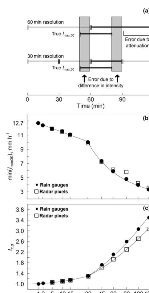
de-creased pronouncedly when resolution dede-creased from 1 min down to 120 min (by 1, 14 and 16 % at a resolution of 2, 60 and 120 min, respectively). To avoid this loss of events, min(Imax30)τ was decreased continuously with decreasing temporal resolution (Fig. 2b). The decrease was less steep below a temporal resolution of 30 min than above:
min(Imax30)= −0.59τ0.5+13.23 forτ≤30 min, (6a)
min(Imax30)=147τ−0.79 forτ >30 min. (6b)
This change at a resolution of 30 min is because 30 min is the time interval in which the maximum is searched for. For reso-lutions higher than 30 min, there is a discrepancy between the true period ofImax30and the period ofImax30that is coerced
Figure 2. (a) Time periods influencing the underestimation of
[image:6.612.306.548.81.554.2]by the temporal resolution (see grey bars in Fig. 2a). The error caused by this discrepancy only results from the dif-ference in intensity immediately before and after trueImax30.
When the temporal resolution becomes less than 30 min, at-tenuation caused by the period exceeding the 30 min inter-val additionally decreases in intensity (see 60 min resolution in Fig. 2a). This attenuation increases the lower the tempo-ral resolution becomes, and it caused Eq. (6b) to be much steeper than Eq. (6a).
The decrease in min(Imax30)τ was identical for both the rain gauge scale and the 1 km2 scale (slope between both scales: 1.0067, r2=0.9858, n=9). For both scales com-bined, RMSE was only 0.10 and 0.39 for Eq. (6a) and (6b), respectively. Thus, both equations were valid for point scale and for a grid width of 1 km.
Rain erosivity also decreased with decreasing temporal resolution; in turn, the scaling factortτ,σ increased (Fig. 2c; Eq. 7a–7c). For intervalsτ≤30 min, the increase was iden-tical for rain gauge scale and for radar pixels of 1 km pixel width. The increase of tτ,σ was much steeper when τ be-came longer than 30 min. This increase then depended on the spatial scale and was larger for rain gauge scale than for radar pixels of 1 km pixel width (Fig. 2c). The behaviour of
tτ,σ was caused by underestimatingEkinand
underestimat-ing Imax30. The underestimation ofImax30was the stronger
effect (data not shown). It prevailed for time intervals greater than 30 min and caused the break at a temporal resolution of 30 min, as already shown for min(Imax30)τ. The identical be-haviour of intensity with decreasing temporal resolution at rain gauge scale and at 1 km2radar pixel scale that was al-ready evident for min(Imax30)τ thus also led to identicaltτ,σ for both spatial scales as long asτ was less than 30 min. For
τ >30 min the attenuation of intensity peaks came into play. This attenuation was less for the 1 km radar data than for the rain gauge data because the time a moving intensity peak re-mains in a 1 km2grid pixel is longer than the time it requires to pass a rain gauge. In consequence, three equations fortτ,σ (Eq. 7a–7c) were necessary to adjustRe,Ryor R to 1 min
resolution at the respective spatial scale.
Forτ≤30 min and point or 1×1 km2grid scale:
tτ,σ =
τ
100+1 (7a)
Forτ≥30 min and point scale or:
tτ,σ=0=
τ
40+0.55 (7b)
Forτ≥30 min and 1×1 km2grid scale:
tτ,σ=1=
τ
50+0.70 (7c)
The RMSE of all three equations was less than 0.04. The validity of combining the effects of min(Imax30)τ=60 and
tτ=60,σ=1 was supported by the close correlation of
[image:7.612.320.535.61.269.2]tem-porally scaled Ry derived from 5 and 60 min RADOLAN
Figure 3.Spatial scaling factors for long-term average annualR. Open circles result from rain gauges aggregated to pseudo-radar pixels. Open squares result from radar and aggregation of radar data. Error bars represent the 95 % confidence interval. Lines denote a multiple regression (see text). Thexaxis is square-root-scaled to improve visibility at low pixel width.
data, for which the Nash–Sutcliffe efficiency was 0.9483 (n=1568) while RMSE was 8.8 N h−1yr−1.
Variation among monthly tτ,σ=0 was small, especially
forτ≤60 min. The coefficient of variation among monthly
tτ,σ=0was≤6 % forτ ≤60 min and 11 % to 14 % forτ >
60 min. It was not clear if there was seasonality in this varia-tion because for some temporal resoluvaria-tionstτ,σ=0was higher
for summer than for winter months, while for other resolu-tions the opposite was the case.
There was also a negligible regional variation for τ >
30 min, while no difference could be found forτ ≤30 min. For intervals longer than 30 min the scaling factortτ,σ=0
in-creased slightly more in northern Germany (+4 %) than in southern Germany (−2 %), compared to the whole of Ger-many. This small difference will only become relevant if data of very low temporal resolution are used.
3.2 Spatial-scale effects
Erosivities from all data of rain gauge–radar pixel pairs were calculated by application of appropriate min(Imax30)τ and temporal scaling factors to enable comparison. Annual ero-sivity Ry for the 0.5×0.5 km2 pseudo-radar data set was
7.3 % lower than the averageRyof the rain gauges. This
re-sulted in a factorsσ=0.5of 1.08 (CI: 1.00–1.16). This factor
increased tosσ=1=1.15 (CI: 1.04–1.26) whenRywas
cal-culated from 1×1 km2pseudo-radar data (Fig. 3).
Table 2.Percentage of cases that were erosive at point (115 rain gauges) or pixel scale (115 radar pixels) relative to a total of 35 124 point–pixel pairs of rain events that were erosive on at least one of both scales.
Point scale Pixel scale Percentage
Erosive Not erosive 27 %
Not erosive Erosive 16 %
Erosive Erosive 57 %
and 223 N h−1yr−1 over 16 years and was on average 90.2 N h−1yr−1. For the radar pixels, R varied between 26 and 146 N h−1yr−1but was on average only 62 N h−1yr−1 (Fig. 4). In this case the deviation was equal to a factor of 1.48 (CI: 1.43–1.52), which was considerably larger than
sσ=1obtained from pseudo-radar data, for which no
differ-ence in measurement method occurred between point scale and pixel scale. This difference was hence assigned to a method effect (Fig. 3).
The monthly comparison of the 115 rain gauge–radar pixel pairs over 16 years did not yield significant differences be-tween months due to the large CI of the combined scale and method effects (CI between±4 % and±9 % for the individ-ual months), but on average this combined effect was lower during the hydrological winter months (1.16; CI: 1.12–1.21) than during the hydrological summer months (1.42; CI: 1.30– 1.53). This difference, despite being significant (p <0.001), was unimportant because of the small contribution of winter months to annual erosivity.
For the large and contiguous radar data set of 800× 600 pixels, 1.9×10⁶events were recorded at 1×1 km2scale. For these events, Re was on average 5.1 N h−1 and ranged
from 0.5 to 1270 N h−1. Aggregating these pixels to larger square pixels decreased Re. At 18×18 km2, Re was on
average 4.4 N h−1 and ranged from 0.2 to 221.6 N h−1. In consequence, the spatial scaling factorsσ increased further (Fig. 3). The increase in scaling factors over the entire range from point scale to 18 km grid width could be described by a multiple regression (r2=0.9995,n=21) accounting for pixel width σ (in km) and the method effectm depending on the methodµ(which is 0 for rain gauges and 1 for radar data):
m+sσ=1+0.35µ+0.092σ3/4. (8) The CI was ±0.004 for the slope of σ and±0.02 for the method effect.
[image:8.612.89.246.118.172.2]On average for the pseudo-radar pixel, rain was erosive for only 10 out of 12 rain gauges. Hence only 83 % of the 1 km2 pixel was covered by an erosive event. The fraction covered by the erosive event decreased further the larger the pixel size became (fraction=83 %−10.3×ln(pixel size (km2)),r2= 0.9974,n=18). On average only about 50 % of a 5×5 km2 pixel and 25 % of a 17×17 km2pixel received an erosive rain event. This makes it increasingly difficult to detect erosive
Figure 4.Annual erosivityRy(grey points) and multi-annual mean erosivityR(black circles) derived from radar pixel and rain gauge data for 115 point–pixel pairs and 16 years. The difference in slope between the solid line and unity (dashed line) is due to the spatial scale and method effects.
rains the larger pixel size becomes.This caused the strong increase in the spatial scaling factor and indicated a strong positional effect.
3.3 Positional effects
The positional effect as defined here describes the variabil-ity of Re within 1×1 km2. Using the pairs with the true
radar data, 29 610 erosive rain events were recorded dur-ing 16 years at the 115 rain gauges. On average,Re was
5.6 N h−1 and ranged from 0.1 to 547.2 N h−1. For the cor-responding 115 radar pixels, 25 884 erosive events were recorded during the 16 years. MeanRe was 4.4 N h−1 and
ranged from 0.2 to 318.9 N h−1.
Combining all events of the 115 rain gauge–radar pixel pairs during 16 years that were at least erosive at rain gauge scale or at radar pixel scale resulted in 35 124 events. Only 57 % of them were erosive at both scales, while the crite-ria for an erosive event were met exclusively at pixel scale for 16 % of all events and exclusively at rain gauge scale for 27 % of all events (Table 2). The gradients of erosivity within 1 km2 were huge. The largest event that was recorded at a rain gauge while the radar pixel indicated no erosive event was 156 N h−1. The largest event for the opposite case, i.e. that radar recorded an erosive event while the rain gauge recorded no erosive event, was similarly high (180 N h−1). The meanRe of erosive events which were recorded for the
Table 3.Percentage of cases that were erosive at point (rain gauge) or pixel scale, using the pseudo-radar data; in total 579 point–pixel pairs of rain events were erosive on at least one of both scales.
Point scale Pixel scale Percentage
Erosive Not erosive 9 %
Not erosive Erosive 6 %
Erosive Erosive 85 %
zero was 2.9 N h−1(SD:±4.9 N h−1). The meanReof events
which were erosive at a rain gauge but not for the correspond-ing radar pixel was also 2.9 N h−1(SD:±5.6 N h−1).
The percentage of unpaired events was not significantly related to the geographical location, neither longitude (r= −0.02,p=0.23) nor latitude (r= −0.01,p=0.83). It was also independent of the distance to the adjacent radar sta-tion (r= −0.02,p=0.79), which might be used as a proxy for increasing noise in the radar data. The percentage was higher in winter (October–March) with 34 % (SD:±2.4 %) than in summer (April–September) with 25 % (SD:±2.4 %). The probability of remaining just below the threshold of an erosive event on one of both scales was higher in winter than in summer as in general winter events are less intensive than summer events. MeanRein winter was only 35 % of mean
Rein summer.
Rain gaugeRewas larger than radarRefor 74 % of those
point–pixel pairs (points above the line of unity in Fig. 5) which were erosive on both scales (19 944 events). MeanpRe was 1.54 (CI:±0.01) for these events. This value quantifies the mean deviation of all locations within a 1 km2pixel that experience a higher erosivity than the mean. For individual locations, the deviation can be much larger, which was al-ready evident from the magnitude of the largest events that were recorded only on one of both scales. For individual locations with an erosive event on both scales, pRe could be considerably higher than 10 (see “outliers” in Fig. 5). Rain gaugeRewas lower than radarRefor only 26 % of all
events (points below the line of unity in Fig. 5), andpRewas 0.72 (CI:±0.01). Again, the deviation of individual locations within 1 km2could be much larger.
For the dense rain gauge field used to create pseudo-radar data, 579 point–pixel pairs of events were at least erosive at rain gauge scale or at pseudo-radar pixel scale. For these 579 events, Re derived from rain gauge data ranged from 0 to
45.5 N h−1(mean: 3.9 N h−1), andRederived from
pseudo-radar data ranged from 0 to 28.1 N h−1 (mean: 3.4 N h−1) (Fig. 6). For 9 % of these events, the event was not erosive with pseudo-radar but at the rain gauge, and for 6 % the op-posite was true (Table 3).
For 67 % of those events which were erosive at both scales, rain gaugeRewas larger than pseudo-radarReandpRe was 1.28 (CI: 1.25–1.30). For 33 % of these events, rain gaugeRe
[image:9.612.87.247.108.163.2]was lower than pseudo-radarReandpRewas 0.81 (CI: 0.77–
Figure 5.Comparison of event erosivityRecalculated from radar data andRefrom rain gauge data for 115 radar pixels that enclose a rain gauge. Only events that were erosive at both scales (19 944 events) during the 16-year period are shown. The dashed line repre-sents unity. Axes are log-scaled. Note that no spatial scaling factor or method factor was applied because these factors also included the effect of incomplete coverage of the pixel by an erosive rain cell.
0.85). Also in this case, where measurement errors could be excluded because rain gaugeRe and pseudo-radarRe were
calculated from the same data, the variation within 1 km2was again huge. For the single days with erosive events,Revaried
greatly between rain gauges. For an example see height of the rectangle in Fig. 6. Although this was the largest event in this data set, one rain gauge remained below the threshold and hence recorded no erosive event. This large variation was also reflected by the large coefficient of variation between rain gaugeRefor the same day (mean: 68 %).
4 Discussion
Figure 6. Event erosivity Re at 12 rain gauges located within a 1 km2pixel vs.Rebased on pseudo-radar data calculated from the hyetographs of the 12 rain gauges (open grey circles). Filled black circles show the averageReof all 12 rain gauges vs. theRefrom pseudo-radar rainfall. Note that the average Re can be consider-ably larger than zero while the averaged rainfall of the pseudo-radar remains below the thresholds of erosivity (black circles along the
yaxis). Rectangular frame shows variation ofRefor a single day. Axes are square-root-scaled to improve resolution at lowRe.
al., 2016). Erosivity can thus reliably be recorded at the po-sition of a rain gauge, but this information cannot even be extrapolated over a distance of only 500 m (half of our radar pixel widths). This was illustrated by the fact that, within this distance, Re could be zero or>150 N h−1, which is more
than twice the annual erosivity in Germany (Auerswald, 2006; Sauerborn, 1994). It is also illustrated by the fact that the largest Re that was recorded within only 2 months
was 1270 N h−1when contiguous measurements were used, while the largest Re that occurred during 16 years when
the same region was covered by 115 rain gauges was only 547 N h−1. Hence rain gauge measurements fail to record many erosive events that occur in their close vicinity (even
<500 m). Erosivity determined by a rain gauge cannot be extrapolated to a small watershed, to farms or even to fields. Discrepancies between model predictions and measurements of erosion that can be found in many studies (Govers, 1991; Liu et al., 1997; Risse et al., 1993; Rüttimann et al., 1995; Zhang et al., 1996) probably originate in part from this strong positional effect. Such strong discrepancies during individual events even exist between replicates of bare plots (Nearing et al., 1999) or between replicated vegetated plots and cannot be explained by plot characteristics. They do not appear in sub-sequent runoff and soil loss observations (Wendt et al., 1986).
Erosion prediction and model development are thus strongly limited by the unexplained variability caused by short-range erosivity gradients. Hence, there is no alternative to using contiguous rain measurements. Radar technology provides, for the first time, measurements that fulfil this need.
Contiguous measurements, on the other hand, suffer from the fact that they cannot be carried out at the same temporal and spatial scale as rain gauge measurements, and the method of measurement differs. Here we provide scaling factors that help to partly overcome this problem and that allow radar measurements to be used for erosivity calculations. These factors, however, do not solve the problem that contiguous measurements integrate over a certain space and time and thus that the information about the variation within these do-mains is lost. In particular, the positional effect can only be used to quantify uncertainty within a radar pixel, but it can-not be used to predict erosivity at specific locations within a pixel. This large uncertainty is probably also one of the main reasons for the discrepancy between observed soil loss and predicted soil loss based on radar rain data for individ-ual fields, whereas this discrepancy disappeared as soon as many fields were grouped, irrespective of how this group-ing was done (Fischer et al., 2018a; Auerswald et al., 2018). With future improvements in technology it may become pos-sible to further improve temporal and spatial resolution of contiguous rain data and, thus, to reduce the uncertainty of event erosivities.
Temporal scaling factors had already been developed (Auerswald et al., 2015; Agnese et al., 2006; Istok et al., 1986; Williams and Sheridan, 1991; Weiss, 1964; Yin et al., 2007) because they are also required for rain gauge measure-ments of low temporal resolution (in data storage). Our tem-poral scaling factors were of a similar order of magnitude to those in other studies. However, our data showed that using a scaling factor is not sufficient because the intensity thresh-old also has to be adjusted in order to identify the correct number of erosive events. The existence of an erosive event and long-term sums of erosivity will otherwise be incorrect, even with a temporal scaling factor. To our knowledge our study provides, for the first time, a function that enables the intensity threshold to be adjusted according to the temporal resolution of the rain data. Adjustment of the total rain depth threshold is not necessary because total rain depth should be independent of the temporal resolution, as long as it is still short enough to identify the rain breaks that separate individ-ual events.
Despite providing intensity thresholds and scaling factors forRe,RyandRfor different temporal resolutions, we
time increments, only compensation for the error that re-sulted from an imperfect identification of the period ofImax30
was necessary. Longer time increments than 30 min addition-ally attenuatedImax30and thus blurred this information.
The spatial scale was more difficult to consider than the temporal scale due to the large positional effect. In particular, large parts of a pixel remained below the thresholds of an ero-sive event even when measurement errors could be excluded, like in the case of the pseudo-radar pixel that used rain gauge measurements. On average, 17 % of the rain gauges within a 1 km2pixel remained below the erosivity threshold while the other rain gauges recorded an erosive event. This percent-age increased strongly with increasing pixel size. In conse-quence, the spatial-scale effect cannot be corrected for indi-vidual events but only for the averages of many events.
The spatial scaling factor is conceptually the inverse of the so-called areal reduction factors, which are used to reduce rain intensity from rain gauge measurements when scaled to catchment areas depending on the duration and return period of the rain event (Allen and DeGaetano, 2005; De Michele et al., 2001; Stewart, 1989). This conceptual difference is due to the difference in the intended purpose of contiguous rain data. While in catchment hydrology the average and the rela-tive distribution of rain depth within a watershed is of interest (Asquith and Famiglietti, 2000), for erosion analysis rain in-tensities are important at point and field scale, where erosion occurs.
The method effect combines all differences in measure-ment and measuring errors (e.g. the wind effect in the case of rain gauges). It is thus highly dependent on the specific configuration of rain gauge measurements and radar mea-surements, including all subsequent data manipulation steps. These configurations are usually fairly standardized within a country (e.g. rain gauge height and diameter are usually defined) but differ from country to country. Our method ef-fect may thus only be valid for Germany, whereas applica-tion to other countries, even if they use similar rain gauge and radar protocols (e.g. Goudenhoofdt and Delobbe, 2016; Koistinen and Michelson, 2002), should be done with care. The same is true for using satellite data or data of commercial microwave links, which recently have been identified as addi-tional source for retrieving precipitation (Chwala et al., 2012; Overeem et al., 2013) and which will require the method ef-fect to be adapted for this particular approach. The approach is based on analysing the signal attenuation that depends on rain intensity. These data are especially valuable in regions with sparse coverage by conventional measurement devices, e.g. in parts of the African continent, but may also improve high-resolution precipitation estimates and forecasts in hy-drometeorological applications (Chwala et al., 2016).
As an example, for the new German RADOLAN product that recently became publicly available (spatial resolution: 1 km2; temporal resolution: 60 min) theImax30threshold has
to be lowered to 5.79 mm h−1, while the total precipitation threshold remains at 12.7 mm. The temporal scaling factor
becomest=1.9, and the spatial scaling factor becomess= 1.13, to which the method effect ofm=0.35 has to be added. In total, the correction factor is 2.81((1.13+0.35)×1.9). Hence the change of theImax30threshold and the combined
scaling factor are large, and ignoring both would consider-ably underestimate erosivity. The large change of theImax30
threshold and the large temporal scaling factor also show that much information is lost when using data of 60 min resolu-tion.
This loss of information can be either an advantage or a disadvantage. It would be a disadvantage in hindcasting, wherein usually the true pattern of erosivity is wanted. In this case a better-resolved product like 5 min data should be used. TheImax30threshold would then be 11.9 mm h−1, and
the temporal scaling factor would only bet=1.05, indicat-ing a minor loss of information. The spatial scalindicat-ing factor is already rather low, and the method effect cannot be avoided. On the other hand the loss of information would be an advantage in forecasting, which aims at the likely regional pattern of erosivity. The loss of information removes the in-fluence of randomly occurring local events of extraordinarily high magnitude that add noise to the regional pattern of ero-sivity. The finding that the largestRe within only 2 months
was 1270 N h−1while the expected long-term averageRwas only about 70 N h−1yr−1(Sauerborn, 1994) shows that this single event would add 64 N h−1yr−1to a 20-year record of radar data. Even in a 100-year record this single event would still be detectable. Using data of 60 min resolution thus re-duces the need for smoothing the map statistically to remove the influence of such local events.
5 Conclusions
Large gradients in event erosivity occur that can only be cap-tured by contiguous rain data. Radar technology enables such contiguous rain data to be recorded but not at the same tem-poral and spatial scale as measurements from rain gauges. Using data of lower temporal and spatial resolution than rain gauges leads to a pronounced underestimation of erosivity. Here we provide a set of correction functions that enable this underestimation to be corrected. In particular, the intensity threshold has to be modified, and a temporal scaling factor, a spatial scaling factor and a factor accounting for measure-ment peculiarities have to be considered. In combination with contiguous radar rain data this could be a major step forward in erosion modelling.
Author contributions. KA and FKF designed the analysis, which was mainly carried out by FKF. TW provided most data and the knowledge about all steps involved in radar data creation. FKF and KA prepared the manuscript with contributions by TW.
Competing interests. The authors declare that they have no conflict of interest.
Acknowledgements. This study was part of the project “Ermittlung des Raum- und Jahreszeitmusters der Regenerosivität in Bayern aus radargestützten Niederschlagsdaten zur Verbesserung der Erosionsprognose mit der Allgemeinen Bodenabtragsgleichung” at the Bavarian State Research Center for Agriculture (PI Robert Brandhuber) and funded by the Bayerisches Staatsministerium für Ernährung, Landwirtschaft und Forsten (A/15/17). Karin Levin provided language editing.
This work was supported by the German Research Foundation (DFG) and the Technische Universität München within the funding programme Open Access Publishing.
Edited by: Nunzio Romano
Reviewed by: two anonymous referees
References
Agnese, C., Bagarello, V., Corrao, C., D’Agostino, L., and D’Asaro, F.: Influence of the rainfall measurement interval on the erosivity determinations in the Mediterranean area, J. Hydrol., 329, 39–48, https://doi.org/10.1016/j.jhydrol.2006.02.002, 2006.
Allen R. J. and DeGaetano, A. T.: Areal reduction factors for two eastern United States regions with high rain-gauge density, J. Hy-drol. Eng., 10, 327–335, https://doi.org/10.1061/(ASCE)1084-0699(2005)10:4(327), 2005.
Asquith, W. H. and Famiglietti, J. S.: Precipitation areal-reduction factor estimation using an annual-maxima centered ap-proach, J. Hydrol., 230, 55–69, https://doi.org/10.1016/S0022-1694(00)00170-0, 2000.
Auerswald, K.: Germany, in: Soil Erosion in Europe, edited by: Boardman, J. and Poesen, J., Wiley, 213–230, https://doi.org/10.1002/0470859202.ch18, 2006.
Auerswald, K., Fiener, P., Gomez, J. A., Govers, G., Quin-ton J. N., and Strauss, P.: Comment on “Rainfall ero-sivity in Europe” by Panagos et al. (Sci. Total Environ., 511, 801–814, 2015), Sci. Total Environ., 532, 849–852, https://doi.org/10.1016/j.scitotenv.2015.05.019, 2015.
Auerswald, K., Fischer, F. K., Kistler, M., Treisch, M., Maier, H., and Brandhuber, R., Behavior of farmers in regard to erosion by water as reflected by their farming practices, Sci. Total Environ., 613–614, 1–9, https://doi.org/10.1016/j.scitotenv.2017.09.003, 2018.
Bartels, H., Weigl, E., Reich, T., Lang, P., Wagner, A., Kohler, O., and Gerlach, N.: Projekt RADOLAN: Routineverfahren zur Online-Aneichung der Radarniederschlagsdaten mit Hilfe von automatischen Bodenniederschlagsstationen (Ombrometer),
Deutscher Wetterdienst, Hydrometeorologie, Offenbach/M., available at: http://www.laenderfinanzierungsprogramm.de/ cms/WaBoAb_prod/WaBoAb/Vorhaben/LAWA/Vorhaben_ des_ehemaligen_Ausschusses_Daten/DK_5.68/RADOLAN_ Abschlussbericht_2006.pdf (last access: 12 December 2017), 2004.
Chen, C.-T. and Knutson, T.: On the verification and comparison of extreme rainfall indices from climate models, J. Climate, 21, 1605–1621, https://doi.org/10.1175/2007JCLI1494.1, 2008. Christensen, O. B., Drews, M., Christensen, J. H., Dethloff,
K., Ketelse, K., Hebestadt, I., and Rinke, A.: The HIRHAM Regional Climate Model Version 5 (beta). Danish Climate Centre, Danish Meteorological Institute, Technical Report; No. 06-17, available at: http://orbit.dtu.dk/en/publications/the- hirham-regional-climate-model-version-5-beta(1fc11ce7-0e59-4179-8ecc-e9233f2bbe4b).html (last access: 14 May 2018), 2007.
Chwala, C., Gmeiner, A., Qiu, W., Hipp, S., Nienaber, D., Siart, U., Eibert, T., Pohl, M., Seltmann, J., Fritz, J., and Kunstmann, H.: Precipitation observation using microwave backhaul links in the alpine and pre-alpine region of Southern Germany, Hydrol. Earth Syst. Sci., 16, 2647–2661, https://doi.org/10.5194/hess-16-2647-2012, 2012.
Chwala, C., Keis, F., and Kunstmann, H.: Real-time data acquisition of commercial microwave link networks for hydrometeorological applications, Atmos. Meas. Tech., 9, 991– 999, https://doi.org/10.5194/amt-9-991-2016, 2016.
Dabney, S. M., Yoder, D. C., and Vieira, D. A. N.: The applica-tion of the revised universal soil loss equaapplica-tion, version 2, to evaluate the impacts of alternative climate change scenarios on runoff and sediment yield, J. Soil Water Conserv., 67, 343–353, https://doi.org/10.2489/jswc.67.5.343, 2012.
De Michele, C., Kottegoda, N. T., and Rosso R.: The derivation of areal reduction factor of storm rainfall from its scaling properties, Water Resour. Res., 37, 3247–3252, https://doi.org/10.1029/2001WR000346, 2001.
Fairman, J. G., Shultz, D. M., Kirshbaum, D. J., Hray, S. L., and Barrett, A. I.: A radar-based rainfall climatol-ogy of Great Britain and Ireland, Weather, 70, 153–158, https://doi.org/10.1002/wea.2486, 2015.
Fiener, P. and Auerswald, K.: Spatial variability of rainfall on a sub-kilometre scale, Earth Surf. Process. Landf., 34, 848–859, https://doi.org/10.1002/esp.1779, 2009.
Fischer, F., Hauck, J., Brandhuber, R., Weigl, E., Maier, H., and Auerswald, K.: Spatio-temporal variability of erosivity estimated from highly resolved and adjusted radar rain data, Agr. Forest Meteorol., 223, 72–80, https://doi.org/10.1016/j.agrformet.2016.03.024, 2016.
Fischer, F. K., Kistler, M., Brandhuber, R., Maier, H., Treisch, M., and Auerswald, K.: Validation of official erosion mod-elling based on high-resolution radar rain data by aerial photo erosion classification, Earth Surf. Proc. Land., 43, 187–194, https://doi.org/10.1002/esp.4216, 2018a.
Flato, G., Marotzke, J., Abiodun, B., Braconnot, P., Chou, S. C., Collins, W., Cox, P., Driouech, F., Emori, S., Eyring, V., Forest, C., Gleckler, P., Guilyardi, E., Jakob, C., Kattsov V., Reason, C., and Rummukainen, M.: Evaluation of cli-mate models, in: Clicli-mate Change 2013: The Physical Sci-ence Basis. Contribution of Working Group I to the Fifth As-sessment Report of the Intergovernmental Panel on Climate Change, edited by: Stocker, T. F., Qin, D., Plattner, G.-K., Tignor, M., Allen, S. K., Boschung, J., Nauels, A., Xia, Y., Bex, V., and Midgley, P. M., Cambridge University Press, Cambridge, United Kingdom and New York, NY, USA, 741– 866, available at: https://www.ipcc.ch/pdf/assessment-report/ ar5/wg1/WG1AR5_Chapter09_FINAL.pdf (last access 14 May 2018), 2013.
Goudenhoofdt, E. and Delobbe, L.: Generation and verifica-tion of rainfall estimates from 10-yr volumetric weather radar measurements, J. Hydrometeorol., 17, 1223–1242, https://doi.org/10.1175/JHM-D-15-0166.1, 2016.
Govers, G.: Rill erosion on arable land in central Bel-gium: rates, controls, and predictability, Catena, 18, 133–155, https://doi.org/10.1016/0341-8162(91)90013-N, 1991.
Habib, E., Krajewski, W. F., and Kruger, A.: Sampling errors of tipping-bucket rain gauge measurements, J. Hydrol. Eng., 6, 159–166, 2001.
Hardegree, S. P., Van Vactor, S. S., Levinson, D. H., and Winstral, A. H.: Evaluation of NEXRAD radar precipitation products for natural resource applications, Rangeland Ecol. Manag., 61, 346– 353, doi 10.2111/07-036.1, 2008.
Istok, J. D., McCool, D. K., King, L. G., and Boersma, L.: Effect of rainfall measurement interval on EI calculation, T. ASAE, 29, 730–734, https://doi.org/10.13031/2013.30221, 1986.
Kaspar, F., Müller-Westermeier, G., Penda, E., Mächel, H., Zim-mermann, K., Kaiser-Weiss, A., and Deutschländer, T.: Monitor-ing of climate change in Germany – data, products and services of Germany’s National Climate Data Centre, Adv. Sci. Res., 10, 99–106, https://doi.org/10.5194/asr-10-99-2013, 2013.
Koistinen, J. and Michelson, D. B.: BALTEX weather radar-based precipitation products and their accuracies, Boreal Environ. Res., 7, 253–263, 2002.
Krajewski, W. F., Ciach, G. J., and Habib, E.: An analysis of small-scale rainfall variability in differ-ent climatic regimes, Hydrolog. Sci. J., 48, 151–162, https://doi.org/10.1623/hysj.48.2.151.44694, 2003.
Liu, B. Y., Nearing, M. A., Baffaut, C., and Ascough II, J. C.: The WEPP watershed model: III. Comparisons to mea-sured data from small watersheds, T. ASAE, 40, 945–951, https://doi.org/10.13031/2013.21345, 1997.
Michelson, D., Szturc, J., Gill, R. S., and Peura, M.: Community-based weather radar networking with BALTRAD, The sixth Eu-ropean Conference on Radar in Meteorology and Hydrology ERAD Proceedings, 6 pp., available at: http://www.erad2010. com/pdf/oral/wednesday/dataex/01_ERAD2010_0170.pdf (last access: 14 May 2018), 2010.
Nash, J. E. and Sutcliffe, J. V.: River flow forecasting through con-ceptual models. Part I. A discussion of principles, J. Hydrol., 10, 282–290, https://doi.org/10.1016/0022-1694(70)90255-6, 1970. Nearing, M. A., Govers, G., and Norton, L. D.: Variability in soil
erosion data from replicated plots, Soil Sci. Soc. Am. J., 63, 1829–1835, https://doi.org/10.2136/sssaj1999.6361829x, 1999.
Nearing, M. A., Yin, S.-Q., Borrelli, P., and Polyakov, V. O.: Rainfall erosivity: An historical review, Catena, 157, 357–362, https://doi.org/10.1016/j.catena.2017.06.004, 2017.
Overeem, A., Leijnse, H., and Uijlenhoet, R.: Country-wide rainfall maps from cellular communication networks, P. Natl. Acad. Sci. USA, 110, 2741–2745, 2013.
Pedersen, L., Jensen, N. E., Christensen, L. E., and Madsen, H.: Quantification of the spatial variability of rainfall based on a dense network of rain gauges, Atmos. Res., 95, 441–454, https://doi.org/10.1016/j.atmosres.2009.11.007, 2010.
Peleg, N., Marra, F., Fatichi, S., Paschalis, A., and Molnar, P.: Spatial variability of extreme rainfall at radar subpixel scale, J. Hydrol., 556, 922–933, https://doi.org/10.1016/j.jhydrol.2016.05.033, 2016.
Risse, L. M., Nearing, M. A., Nicks, A. D., and Laflen, J. M.: Error assessment in the universal soil loss equation, Soil Sci. Soc. Am. J., 57, 825–833, https://doi.org/10.2136/sssaj1993.03615995005700030032x, 1993.
Rüttimann, M., Schaub, D., Prasuhn, V., and Rüegg, W.: Measure-ment of runoff and soil erosion on regularly cultivated fields in Switzerland – some critical considerations, Catena, 25, 127–139, https://doi.org/10.1016/0341-8162(95)00005-D, 1995.
Rogler, H. and Schwertmann, U.: Erosivität der Niederschläge und Isoerodentkarte Bayerns, J. Rural Engi. Developm., 22, 99–112, 1981.
Sauerborn, P.: Die Erosivität der Niederschläge in Deutschland. Ein Beitrag zur quantitativen Prognose der Bodenerosion durch Wasser in Mitteleuropa, Bonner Bodenkundliche Abhandlungen, 13, 189 pp., 1994.
Spengler, R.: The new quality control and monitoring system of the Deutscher Wetterdienst, Proceedings of the WMO Technical Conference on Meteorological and Environmental Instruments and Methods of Observation, Bratislava, 2002.
Stewart, E. J.: Areal reduction factors for design storm construc-tion: Joint use of raingauge and radar data, International Associ-ation of Hydrological Sciences Publ., 181, 31–49, available from IAHS, Centre for Ecology and Hydrology, Wallingford, Oxford-shire OX108BB, UK, 1989.
USDA-Agricultural Research Service: Science Documentation Revised Universal Soil Loss Equation Version 2, available at: https://www.ars.usda.gov/ARSUserFiles/60600505/rusle/ rusle2_science_doc.pdf (last access: 14 May 2018), 2013. Vrieling, A., Sterk, G., and de Jong, S. M.: Satellite-based
estima-tion of rainfall erosivity for Africa, J. Hydrol., 395, 235–241, 2010.
Vrieling, A., Hoedjes, J. C. B., and van der Velde, M.: Towards large-scale monitoring of soil erosion in Africa: Accounting for the dynamics of rainfall erosivity, Global Planet. Change, 115, 33–43, 2014.
Vuerich, E., Monesi, C., Lanza, L., Stagi, L., and Lanzinger, E.: WMO field intercomparison of rainfall intensity gauges, World Meteorological Organization, IOM Report-No. 99, available at: http://library.wmo.int/pmb_ged/wmo-td_1504.pdf (last access: 11 December 2018), 2009.
Syst. Sci., 16, 4101–4117, https://doi.org/10.5194/hess-16-4101-2012, 2012.
Weiss, L. L.: Ratio of true to fixed-interval maximum rainfall, J. Hydr. Eng. Div-ASCE, 90, 77–82, 1964.
Williams, R. G. and Sheridan, J. M.: Effect of rainfall measurement time and depth resolution on EI calculation, T. ASAE, 34, 402– 406, 1991.
Wendt, R. C., Alberts, E. E., and Hjelmfelt Jr., A. T.: Variability of runoff and soil loss from fallow exper-imental plots, Soil Sci. Soc. Am. J., 50, 730–736, https://doi.org/10.2136/sssaj1986.03615995005000030035x, 1986.
Winterrath, T., Rosenow, W., and Weigl, E.: On the DWD quanti-tative precipitation analysis and nowcasting system for real-time application in German flood risk management, IAHS Red Book, 351, 323–329, 2012.
Winterrath, T., Brendel, C., Hafer, M., Junghänel, T., Klameth, A., Walawender, E., Weigl, E., and Becker, A.: Erstellung einer dekadischen radargestützten hoch-auflösenden Niederschlagskli-matologie für Deutschland zur Auswertung der rezenten Än-derung des Extremverhaltens von Niederschlag, Abschluss-bericht, Deutscher Wetterdienst, Offenbach/M, 2017.
Winterrath, T., Brendel, C., Hafer, M., Junghänel, T., Klameth, A., Lengfeld, K., Walawender, E., Weigl, E., and Becker, A.: RADKLIM Version 2017.002: Reprocessed quasi gauge-adjusted radar data, 5-minute precipitation sums (YW), https://doi.org/10.5676/DWD/RADKLIM_YW_V2017.002, 2018a.
Winterrath, T., Brendel, C., Hafer, M., Junghänel, T., Klameth, A., Lengfeld, K., Walawender, E., Weigl, E., and Becker, A.: RADKLIM Version 2017.002: Reprocessed gauge-adjusted radar data, one-hour precipitation sums (RW), https://doi.org/10.5676/DWD/RADKLIM_RW_V2017.002, 2018b.
Wischmeier, W. H.: A rainfall erosion index for a universal soil-loss equation, Soil Sci. Soc. Am. Proc., 23, 246–249, 1959.
Wischmeier, W. H. and Smith, D. D.: Rainfall energy and its rela-tionship to soil loss, T. Am. Geophys. Un., 39, 285–291, 1958. Wischmeier, W. H. and Smith, D. D.: Predicting rainfall erosion
losses – a guide to conservation planning, U.S. Department of Agriculture, Agriculture Handbook No. 537, Washington, DC, 1978.
Yin, S., Xie, Y., Nearing, M. A., and Wang, C.: Esti-mation of rainfall erosivity using 5- to 60-minute fixed-interval rainfall data from China, Catena, 70, 306–312, https://doi.org/10.1016/j.catena.2006.10.011, 2007.