Rainfall disaggregation for hydrological modeling: is there a need for spatial consistence?

https://doi.org/10.5194/hess-22-5259-2018 © Author(s) 2018. This work is distributed under the Creative Commons Attribution 4.0 License.

Rainfall disaggregation for hydrological modeling: is there a need

for spatial consistence?

Hannes Müller-Thomy1,2,*, Markus Wallner3, and Kristian Förster1,4,5

1_{Institute of Hydrology and Water Resources Management, Leibniz Universität Hannover, 30175 Hanover, Germany} 2_{Institute of Hydraulic Engineering and Water Resources Management, Vienna University}

of Technology, Vienna, 1040, Austria

3_{bpi Hannover – Beratende Ingenieure, 30177 Hanover, Germany}

4_{Institute of Geography, University of Innsbruck, Innsbruck, 6020, Austria} 5_{alpS – Centre for Climate Change Adaptation, Innsbruck, 6020, Austria} *_{previously published under the name Hannes Müller}

Correspondence:Hannes Müller-Thomy ([email protected]) Received: 10 October 2017 – Discussion started: 15 November 2017

Revised: 31 August 2018 – Accepted: 3 September 2018 – Published: 15 October 2018

Abstract.In this study, the influence of disaggregated rain-fall products with different degrees of spatial consistence on rainfall–runoff modeling results is analyzed for three mesoscale catchments in Lower Saxony, Germany. For the disaggregation of daily rainfall time series into hourly val-ues, a multiplicative random cascade model is applied. The disaggregation is applied on a station by station basis with-out consideration of surrounding stations; hence subsequent steps are then required to implement spatial consistence. Spa-tial consistence is represented here by three bivariate spa-tial rainfall characteristics that complement each other. A re-sampling algorithm and a parallelization approach are eval-uated against the disaggregated time series without any sub-sequent steps. With respect to rainfall, clear differences be-tween these three approaches can be identified regarding bi-variate spatial rainfall characteristics, areal rainfall intensi-ties and extreme values. The resampled time series lead to the best agreement with the observed ones. Using these dif-ferent rainfall products as input to hydrological modeling, we hypothesize that derived runoff statistics – with emphasis on seasonal extreme values – are subject to similar differences as well. However, an impact on the extreme values’ statis-tics of the hydrological simulations forced by different rain-fall approaches cannot be detected. Several modifications of the study design using rainfall–runoff models with and with-out parameter calibration or using different rain gauge den-sities lead to similar results in runoff statistics. Only if the

spatially highly resolved rainfall–runoff WaSiM model is ap-plied instead of the semi-distributed HBV-IWW model can slight differences regarding the seasonal peak flows be iden-tified. Hence, the hypothesis formulated before is rejected in this case study. These findings suggest that (i) simple model structures might compensate for deficiencies in spatial rep-resentativeness through parameterization and (ii) highly re-solved hydrological models benefit from improved spatial modeling of rainfall.

1 Introduction

Flood quantiles are important information for the creation of flood hazard maps, the construction of riverfront build-ings and landscape development plans, for example. For un-gauged catchments and catchments with short discharge ob-servation periods, rainfall–runoff modeling is a possibility to obtain long, simulated discharge time series which can then be used for derived flood frequency analysis.

observed rainfall time series of that kind are (i) too short or (ii) the network density is too low. Both are issues because (i) limits the length of the simulation period and hence the derivable flood frequencies and (ii) affects the representation of spatial rainfall patterns (Krajewski et al., 1991; Ogden and Julien, 1993; Obled et al., 1994, and Nicotina et al., 2008) and hence the areal rainfall used as input for the rainfall– runoff simulations.

Usually, time series of daily stations have much longer ob-servation periods and a higher network density. Daily time series can be disaggregated to hourly time series by using information from observed, hourly time series. One possible method for the disaggregation of rainfall is the multiplicative random cascade model (e.g., Olsson, 1998), which was orig-inally introduced within the field of turbulence theory (Man-delbrot, 1974). The use of observed daily time series as in-put is a strong advantage of the cascade model, since start-ing with “true” rainfall amounts and intermittency facilitates their conservation to finer temporal resolutions, while other rainfall generators (e.g., Poisson cluster models; Rodriguez-Iturbe et al., 1987; Onof et al., 2000) try to generate time series with a certain temporal resolution and target statistics without any temporal reference to observations.

With the microcanonical cascade model, the rainfall amount of a coarse time step (e.g., a day) is conserved exactly through the disaggregation process, so that an aggregation of the disaggregated time series would result exactly in the orig-inal observed time series. Starting from a daily resolution, an hourly temporal resolution is achieved, which is a conve-nient input resolution for many rainfall–runoff models. How-ever, this disaggregation method is a univariate process, car-ried out for single time series only which are independent of the time series of surrounding stations. Through the system-atically random distribution of the rainfall amount within a day, unrealistic patterns of rainfall are generated and the spa-tial consistence of rainfall is missing. If an unrealistic spaspa-tial distribution of rainfall is used within a rainfall–runoff simula-tion, it can be assumed that this affects the simulated runoff. However, a realistic spatial representation of rainfall is essen-tial if the time series serve as input for rainfall–runoff mod-eling (e.g., Gires et al., 2015; Paschalis et al., 2014; Ochoa-Rodriguez et al., 2015; Peleg et al., 2017).

Müller and Haberlandt (2015) have introduced a resam-pling scheme as a subsequent step after the disaggregation process, which can be used for the implementation of spatial consistence within disaggregated time series. Spatial consis-tence is hereby defined by three bivariate rainfall character-istics: the probability of occurrence, Pearson’s coefficient of correlation and the continuity ratio (Wilks, 1998). The im-plementation of spatial consistence for hourly time series was proven by the abovementioned bivariate characteristics in ad-dition to areal rainfall intensities resulting from the disaggre-gated time series. Without resampling, areal rainfall intensi-ties were underestimated. The resampling algorithm was ad-ditionally tested for time series of 5 min resolution by Müller

and Haberlandt (2018). Bivariate rainfall characteristics as well as the simulated runoff from an artificial sewage sys-tem were positively validated against observed rainfall time series and its resulting simulated runoff.

Haberlandt and Radtke (2014) overcame the lack of spa-tial consistence using a parallelization approach, which leads to an overestimation of simulated floods, but is preferred in comparison to a possible underestimation. However, Ding et al. (2016) also used disaggregated time series for their rainfall–runoff analyses with a focus on instantaneous peak flows, but without any subsequent changes to the disaggre-gated time series. Neither a systematic over- or underestima-tion of simulated discharge and flood peaks can be found in both investigations.

It can be questioned why the simulation results from both studies, both based upon unrealistic spatial rainfall behavior, lead to an acceptable representation of observed discharge characteristics. The hypothesis of this study is that rainfall products with different degrees of spatial consistence will result in different areal rainfall intensities and hence influ-ence runoff statistics derived from simulated runoff time se-ries. Therefore, three different rainfall products are used as input for rainfall–runoff modeling: disaggregated time se-ries with (Müller and Haberlandt, 2015) and without (Ding et al., 2016) the implementation of spatial consistence, and thirdly, time series with an “overestimated spatial consis-tence” by parallelization (Haberlandt and Radtke, 2014). A systematic comparison is carried out including rainfall– runoff simulations with and without calibration, differing sta-tion densities and different rainfall–runoff models.

In general, calibration and validation of rainfall–runoff model parameters are carried out through a quantitative com-parison of simulated and observed time series. This strategy is not applicable using disaggregated rainfall time series as input, since the daily rainfall amount is distributed randomly in time during a day. Hence, the temporal connection be-tween rainfall and runoff is missing. An alternative strategy is the calibration on runoff statistics and has been applied before by others, for example, Yu and Yang (2000), West-erberg et al. (2011), Haberlandt and Radtke (2014), Wall-ner and Haberlandt (2015) and Ding et al. (2016). Runoff statistics are time-independent, but contain useful informa-tion about the hydrograph and hence about the hydrologi-cal regime and its characteristics. It is assumed that, by a si-multaneous consideration of different complimentary runoff statistics, the runoff behavior can be represented sufficiently. Possible runoff statistics are runoff extremes for different seasons of a year (to take into account, e.g., summer and win-ter floods with their different geneses and resulting runoff be-havior), flow duration curves (to describe the overall behav-ior) and average monthly values (to describe the interannual variability).

Figure 1.Location of all three catchments in the Aller–Leine river basin and its location in Germany.

and the applied rainfall–runoff models including the calibra-tion technique are explained in Sect. 3. Seccalibra-tion 4 includes the results for both the rainfall generation and rainfall–runoff modeling. A summary of the rainfall–runoff model results is provided in Sect. 5 and general conclusions and a brief out-look are provided in Sect. 6.

2 Data and study area 2.1 Catchments

The investigation is carried out for three catchments in the Aller–Leine river basin, namely Reckershausen, Pionier-brücke and Tetendorf (see Fig. 1). The river basin is situ-ated in Lower Saxony, Northern Germany, and has been in-vestigated regarding its runoff extreme values before (e.g., Haberlandt and Radtke, 2014; Ding et al., 2016; Fangmann and Haberlandt, 2018). Based on the Köppen–Geiger climate classification, the river basin can be divided into a temperate oceanic climate in the north and a temperate continental cli-mate in the south (Peel et al., 2007). For Reckershausen an additional investigation regarding rain gauge network den-sity is carried out. All hourly and daily stations for Recker-shausen are shown in Fig. 2.

Figure 2.Reckershausen catchment including sets of three, five and

eight daily stations used for network density analysis.

The catchments differ concerning area and elevation as well as land use and soil conditions. A brief description can be found in Table 1. The soil information is extracted from the soil map BÜK1000 of the Federal Republic of Germany with a scale of 1:1 000 000 (Hartwich et al., 1998). Infor-mation regarding the land use is extracted from the CORINE database (Federal Environment Agency, 2009). The time of concentration has been estimated as per Kirpich (1940).

2.2 Climate data

For the rainfall disaggregation, time series of hourly and daily stations are required. Time series of the hourly stations are used for the parameter estimation of the cascade model (described in Sect. 3.1a), which is in turn used for the disag-gregation of the time series of the daily stations. An overview of rain gauges used in this study is given in Fig. 1, while their measuring periods are given in Table 2. For the daily stations, the chosen period is the longest available period with data for all stations in a catchment. From Table 2 it can be seen that time series have a longer duration for daily stations in com-parison to those for hourly stations for all catchments (up to 2.7 times for Pionierbrücke). Additionally, the number of daily stations is higher.

Table 1.Brief description of the investigated catchments with percentages of dominant soil type and land use.

Catchment River Area Subcatchments Time of concentration Dominant soil type Dominant land use

(km2) (h)

Pionierbrücke Sieber 44 2 1.8 Spodic Cambisols (77 %) Coniferous forest (81 %)

Tetendorf Böhme 110 3 7.2 Haplic Podzols/Dystric Nonirrigated arable land (39 %)

Regosols (40 %)

Reckershausen Leine 321 10 7.4 Dystric Cambisols (37 %) Nonirrigated arable land (59 %)

Table 2.Rain gauges and time series lengths used for each

catch-ment.

Catchment Type Rain gauges Start End

Pionierbrücke Daily 3 1950 2004

Hourly 1 1993 2013

Tetendorf Daily 3 1984 2006

Hourly 1 1993 2013

Reckershausen Daily 8 1972 2006

Hourly 2 1993 2013

The calculation of the potential evaporation is carried out using the Turc–Wendling method on a daily basis (DVWK, 1996). The required sunshine duration per day was derived through ordinary kriging using 29 stations. To achieve an hourly resolution, daily values have been divided by 24, since the inter-daily distribution of potential evaporation has been shown not to be that sensitive as model input. Different land use types have been taken into account by using an average land use parameter (DVWK, 2002) similar to the crop co-efficient. All input data were interpolated and subsequently aggregated to subcatchment scale.

For the WaSiM model, which is only applied for the Pio-nierbrücke catchment, climate time series are needed as point or gridded information on an hourly basis. From the Braun-lage climate station, time series of temperature, relative air humidity and wind speed are available with an hourly resolu-tion. Global radiation was only available on a daily basis, but has been disaggregated to hourly values using an approach as in Förster et al. (2016).

2.3 Runoff data

The available discharge data of the three catchments are listed in Table 3. While observed hourly time series have only been available since 2000 (Pionierbrücke) and 2004 (Tetendorf and Reckershausen), observed extreme values ex-ist for much longer periods. Daily discharge time series exex-ist for at least as long as the period of the hourly extreme values on a monthly basis.

For the calibration, a special focus is given to the extreme values of the summer (1 May–31 October) and winter period (1 November–30 April). Therefore, the maximum observed value of each half year was extracted from both data sources,

Table 3.Available periods of runoff data types.

Catchment Hourly Daily Monthly

discharge discharge extreme time series time series values Pionierbrücke 2000–2013 1929–2006 1952–2005 Tetendorf 2004–2013 1986–2000 1986–2000 Reckershausen 2004–2009 1964–2006 1974–2005

observed hourly time series and monthly extreme values, to generate periods as long as possible.

3 Methods

The method section consists of two subsections. In Sect. 3.1, the multiplicative cascade model for the disaggregation of rainfall time series is explained. Additionally, two methods for the implementation of spatial consistence in the disaggre-gated time series are presented. The descriptions of the two rainfall–runoff models HBV and WaSiM and the calibration procedure for HBV can be found in Sect. 3.2.

3.1 Rainfall generation (a) Rainfall disaggregation

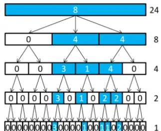
au-Figure 3. General disaggregation scheme of the applied multi-plicative cascade model (values inside the boxes represent rainfall amount, and a blue or white box color indicates wet or dry time steps, respectively).

tocorrelation function also shows underestimations, the ex-treme values are represented well.

(b) Bivariate characteristics

For the definition of spatial consistence applied in this study, the bivariate rainfall characteristics follow the ones used by Haberlandt et al. (2008) and are briefly described in the fol-lowing.

The probability of occurrencePk,ldescribes the

probabil-ity of rainfall occurrence at the same time at two stationsk

andl:

Pk, l(zk>0|zl>0)≈

n11

n , (1)

wherenis the total number of non-missing observation hours at both stations, zi is the rainfall intensity and the number

of simultaneous rainfall occurrence at both stations is repre-sented byn11.

Pearson’s coefficient of correlation ρ describes the rela-tionship between simultaneously occurring rainfall at two stationskandlas a measure of the linear relation between both rainfall time series (Eq. 2). Breinl et al. (2014) used this coefficient before for multisite rainfall generation:

ρk, l=

cov(zk, zl)

√

var(zk)·var(zl)

, zk>0, zl>0. (2)

Müller and Haberlandt (2015) found an intensity dependency for Pearson’s coefficient of correlation and distinguished between ρ(k≤4 mm) and ρ(k >4 mm), which is adopted here.

The continuity ratio Ck, l compares the expected rainfall

amount at one station for times with and without rain at the neighboring station (Eis the expectation operator):

Ck, l=

E (zk|zk>0, zl=0)

E (zk|zk>0, zl>0)

. (3)

Table 4.Short characterization of the three rainfall products.

Starting point Subsequent step Rainfall occurrence Designation

at different stations

Disaggregated None Random V1

time Resampling Intersecting V2

series Parallelization Simultaneous V3

These characteristics are distance-dependent and prescribed values can be estimated as functions of the separation dis-tance between two stations from observed data (see regres-sion lines in Fig. 4 for each characteristic).

(c) Implementation of spatial consistence

As mentioned before, the disaggregation of single time series is a point process with no surrounding stations taken into ac-count. Input rainfall products for the rainfall–runoff models consisting of just the disaggregated time series without sub-sequent steps to implement spatial consistence are referred to as V1 (no implementation of spatial consistence). Two meth-ods for the implementation of spatial consistence, and result-ing in the rainfall products V2 and V3, are applied in this study.

The first method, resulting in V2, is based on simulated annealing (Aarts and Korst, 1965; Kirkpatrick et al., 1983), a nonlinear optimization method from the group of resampling algorithms. The aim of simulated annealing is to modify the disaggregated time series and in doing so minimize an objec-tive function including the deviations between the observed bivariate rainfall characteristics and those from the disaggre-gated time series. Relative diurnal cycles are swapped with-out changing the structure of the time series or the absolute daily totals of rainfall amounts. The interested reader is re-ferred to Müller and Haberlandt (2015) for further details.

The second method, resulting in rainfall product V3, is a more pragmatic solution. It was introduced by Haberlandt and Radtke (2014) and is also based on the time series of V1 that is already disaggregated. For each day, the station with the highest rainfall amount is identified. The relative diurnal cycle of this station is transferred to all other stations for this day. This parallelization is carried out for all days of the dis-aggregated time series. The varying diurnal distributions of rainfall at each station without spatial patterns, leading to an underestimation of spatial consistence, are transformed in-stead to a simultaneous occurrence of rainfall at all stations with an overestimation of spatial consistence.

0 50 100 150 200 250

0.00

0.05

0.10

0.15

0.20

Probability of occurrence

Distance [km]

0 50 100 150 200 250

0.2

0.4

0.6

0.8

1.0

Continuity ratio

Distance [km]

V1 V2 V3

0 50 100 150 200 250

0.2

0.4

0.6

0.8

Coefficient of correlation (≤ 4 mm)

Distance [km]

0 50 100 150 200 250

−0.2

0.0

0.2

0.4

0.6

0.8

Coefficient of correlation (> 4 mm)

Distance [km]

Figure 4.Bivariate spatial rainfall characteristics of V1, V2 and V3 in comparison to observations for the Pionierbrücke catchment (for one

realization, black circles represent observations – for details the reader is referred to Müller and Haberlandt, 2015).

3.2 Hydrological models

For analyzing the impact of rainfall products with different spatial consistencies, two models, HBV-IWW (Wallner et al., 2013) and WaSiM (Schulla, 1997, 2015), are used. All simulations are carried out continuously. This enables the derivation of flood frequency analyses and avoids uncertain-ties from unknown initial conditions resulting from event-based modeling (Pathiraja et al., 2012). Additionally, an ini-tial phase of 1 year is used as a spin-up period to achieve plausible initial conditions for all storages.

(a) HBV-IWW including calibration procedure

The HBV-IWW model is based on the HBV model that was originally developed at the Swedish Meteorological and Hy-drological Institute (SMHI) in the early 1970s (Bergström, 1976) and was modified by Wallner et al. (2013). HBV-IWW, denoted HBV for simplification, is a conceptual model, whereby runoff generation and runoff transformation are rep-resented by simple relationships between storage and effec-tive precipitation, or runoff (see flowchart of the model in Fig. S1 in the Supplement). For the spatial discretization of the study areas, subcatchments (see Fig. 2) with an approx. area of 20 km2are applied. It could be questioned whether a rainfall–runoff model with subcatchments is useful for the validation of the spatial consistence of rainfall. A daily sta-tion covers an area of 65 km2on average in Germany (Müller, 2016). This spatial resolution is not increased by the cas-cade model in this study, since only a temporal disaggre-gation is applied. Also, no additional information is gained by a model with higher spatial resolution. So the only

dis-advantage could be a sort of numerical diffusion due to the spatial resolution. However, since subcatchments of this size are used throughout a number of studies, the HBV with this spatial resolution represents the state of the art and is applied for the current study.

For the estimation of the areal rainfall of each subcatch-ment, a two-step approach was chosen. First, rainfall is in-terpolated with a nearest neighbor approach on a raster basis with cell widths of 1 km. In the second step, areal rainfall for each subcatchment is calculated through the arithmetic mean of all raster cells within the subcatchment. If the areal rainfall of a subcatchment is dominated by one station, it could be questioned whether areal rainfall intensities should be reduced (by, e.g., areal reduction factors; Sivapalan and Blöschl, 1998; Veneziano and Langousis; 2005; Wright et al., 2013) to avoid an overestimation (e.g., Peleg et al., 2018). Since underestimations also occur in the continuous simula-tion if this stasimula-tion was not in the center of the storm, no areal reduction was carried out.

Table 5.Calibration and validation period for all catchments.

Gauge Calibration period Validation period

Start End Start End

Pionierbrücke 1 Nov 1952 31 Oct 1977 1 Nov 1977 31 Oct 2003 Tetendorf 1 Nov 1986 31 Oct 1993 1 Nov 1993 31 Oct 2000 Reckershausen 1 Nov 1974 31 Oct 1990 1 Nov 1990 31 Oct 2006

method. Further details about the model parameters can be found in Wallner et al. (2013) and in Table S2 in the Supple-ment.

For the calibration, the following runoff statistics are used: quantiles of the distribution functions fitted to the extreme values of (i) summer (Extr-Su, May to October) and (ii) win-ter (Extr-Wi, November to April), (iii) quantiles of the flow duration curve (FDC) and (iv) monthly averages (Q-mon). The calibration is carried out for each rainfall product sepa-rately, but for all 10 realizations at the same time (resulting in 1 parameter set for 10 realizations) The calibration procedure is also illustrated in Fig. S1.

For Extr-Su and Extr-Wi, a two-parametric Gumbel distri-bution is fitted to the annual series of extreme values. L mo-ments are used for parameter estimation to reduce the sensi-tivity against outliers (Hosking and Wallis, 1997). Although extreme values only occur in a few time steps, their repro-duction in the discharge time series is the main aim of the simulation on an hourly basis. However, since the extreme values only represent a small fraction of the discharge time series, FDC and Q-mon are also used to represent the more frequent discharge values. Q-mon accounts for the tempo-ral dependency on the interannual variation of the discharge. The analyses of FDC and Q-mon allow no direct validation of the rainfall products, but enable an overall plausible sim-ulation of rainfall–runoff processes. Hence, FDC and Q-mon are calculated from averaged daily discharge values in order to reduce computation time. For the goodness-of-fit analyses of simulated (Sim) and observed (Obs) statistics, the Nash– Sutcliffe-efficiency, NSE (Nash and Sutcliffe, 1970), is used. A perfect fit would result in NSE=1, while assuming the av-erage of the observed data for all time steps would result in NSE=0. The equation for the NSE is given in Eq. (4) and the corresponding quantiles for Extr-Su, Extr-Wi and FDC and months for the Q-mon, respectively, are given in Eq. (5).

NSE=1−

Pn

t=1(QObs(t )−QSim(t ))2

Pn

t=1 QObs(t )−QObs

2 (4)

t= 

      

      

{0.05,0.25,0.5,0.75,0.95,0.975}

for FDC

{1,2,3,4,5,6,7,8,9,10,11,12}

for Q-mon

{0.2,0.5,0.8,0.9,0.95,0.98,0.99}

for Extr-Su and Extr-Wi

(5)

The goodness-of-fit values of all runoff statistics are summa-rized in the objective functionOstat, which should be

mini-mized during the calibration:

Ostat=1−(0.275·NSEExtr-Su+0.275·NSEExtr-Wi

+0.2·NSEFDC+0.25·NSEQ-mon. (6)

For the optimization, simulated annealing is used. The pa-rameters modified during the optimization with the corre-sponding ranges are given in Table S2. The periods for cal-ibration and validation are listed in Table 5 for each catch-ment.

(b) WaSiM

WaSiM (Schulla, 1997, 2015) is a physically based and distributed hydrological model which has been designed to study climate change and land use change impacts on the wa-ter balance and floods in mesoscale catchments (e.g., Niehoff et al., 2002; Bormann and Elfert, 2010). WaSiM was for-merly known as WaSiM-ETH, but has since been renamed (Schulla, 2015), and hence the new abbreviation is used throughout the paper. WaSiM is flexible regarding the res-olution of spatial input data. In general, elevation, land use and soil data need to be prepared as gridded raster datasets. The spatial resolution of WaSiM applications covers several scales ranging from tens of meters to a few kilometers. For this study a spatial resolution of 150 m×150 m was chosen. For the areal rainfall estimation, a combined inverse distance weighting and elevation-dependent regression ap-proach is applied. This apap-proach does not only account for a horizontal interpolation but also addresses the typically observed increase in precipitation with increasing elevation, which proves helpful given that the catchment spans an alti-tudinal range of several hundred meters.

temper-ature threshold for phase partitioning and a tempertemper-ature in-dex model for snowmelt calculations. A bucket approach is applied to consider interception of rainwater. The soil wa-ter dynamics including actual evapotranspiration, infiltration, lateral outflow (interflow) and percolation is simulated in a numerical scheme which is based on the Richards equation. The lowermost nodes in each grid cell, which are subject to saturation, represent the groundwater storage in the model. A linear storage approach is applied here to simulate the out-flow from the groundwater.

Since WaSiM is more complex than HBV with respect to computational needs, a different strategy for model calibra-tion was chosen. As the number of both adjustable param-eters and iterations is limited due to limited computational resources, a lexicographical approach was set up for model calibration (Gelleszun et al., 2017). In this way, the optimiza-tion of parameters is divided into subsequent steps that are associated with different processes. In a first step, the param-eters of the soil water balance and runoff generation (i.e., recession of hydraulic conductivity along the soil profile and the flow density) have been calibrated through maximizing NSE. Then, the baseflow recession is improved through min-imizing the root mean square error of the lowermost part of the flow duration curve (two parameters). Both calibration steps have been performed using hourly meteorological time series and observed discharge time series from the period 2009–2012. As highly resolved meteorological observations are only available from 2000 onwards, an additional calibra-tion step has been carried out using disaggregated rainfall time series in order to better match the long-term water bal-ance characteristics through slightly modifying canopy resis-tance parameters of the evapotranspiration model. Without these pre-calibration steps an underestimation of the mean discharge and hence the water balance was identified. An in-correct representation of the water balance introduces other uncertainty sources, which hence superpose the effects of the different versions of spatial rainfall. However, this pre-calibration was only focused on the water balance itself and not on the objectives used in Eq. (6).

4 Results and discussion

For the discussion of the results, the section is divided into two parts. The first part deals with the interpretation of the rainfall spatial variability, while the influence on simulated discharges is discussed in the second part.

4.1 Rainfall

For the disaggregation of daily rainfall time series to hourly values, the microcanonical cascade model of Müller and Haberlandt (2015) is used. This model was previously val-idated in the aforementioned study for the Aller–Leine river basin, which is also considered in this study. Since the

fo-cus of this study is the spatial variability of the generated rainfall, the interested reader is referred to their investigation for a detailed analysis of point results. In Fig. 4 the bivari-ate characteristics are shown for V1, V2 and V3 in compar-ison with the observations for Pionierbrücke (results for the other two catchments are in Fig. S3 and S4). For the V1 case (the disaggregated time series without any subsequent steps), the probability of occurrence and the correlation coefficients are underestimated, whereas the continuity ratio is overesti-mated.

For the V2 case, the probability of occurrence and the cor-relation coefficients could be improved. While values for the probability of occurrence and correlation coefficient for rain-fall intensities>4 mm are similar to observations, a slight underestimation can be identified for correlation coefficients for rainfall intensities≤4 mm for some station pairs. For the continuity ratio, V2 results vary. This is due to the definition of the criterion, taking stationkwith respect to stationlinto account, but not vice versa. This definition leads to different values for the same station pair because different time steps are taken into account. Therefore, forCk, l an improvement

can be identified during simultaneous worsening ofCl, k.

It should be noted that the resampling algorithm has not been validated in the context of distances smaller than 20 km for hourly time steps. Although the spatial rainfall charac-teristics are underestimated after the disaggregation (V1), a major improvement for all characteristics can be identified by the application of V2, moving all station pairs into the cloud of observations (except some of the continuity ratio).

The simultaneous rainfall of V3 leads to the best values for the continuity ratio, comparable to those from observations. However, slight overestimations can be identified for both coefficients of correlation. For the probability of occurrence, high overestimations can be identified (approximately 50 %). Although the same diurnal cycles are used for all stations, the probability of occurrence is less than 1 due to the fact that rainfall does not necessarily occur at all stations on a wet day.

char-1 2 5 10 20 50

10

20

30

40

50

Pionierbrücke − subcatchment 2

Return period [yr]

R

ai

nf

al

l i

nt

en

si

ty

[m

m

h

]

V1 V2 V3

-1

Figure 5.Annual rainfall extremes of the areal rainfall intensities

for subcatchment 2 in Pionierbrücke. For all 10 realizations used as input for HBV, the solid line represents the median (based on annual extreme values from 1 November 1950 to 31 October 2003).

acteristics and the areal rainfall intensities are consistent. The findings are similar for the other subcatchments in Tetendorf and Reckershausen.

Additionally, the extreme values of the areal rainfall in-tensities have been analyzed, since those can have a sig-nificant influence on the resulting runoff. In Fig. 5, the an-nual maxima rainfall extremes for another subcatchment in Pionierbrücke are illustrated using the Weibull plotting po-sition (similar for all subcatchments). As identified for all areal rainfall intensities, for the extreme values, V1 also leads to the lowest values for each return period. V2 and V3 result in similar values regarding the mean for all re-turn periods. The clear difference of higher values for V3 over the whole spectrum of non-exceedance probability can-not be identified for the extreme values (see Fig. S5). How-ever, for V3, where the diurnal cycle of the station with the highest daily rainfall amount is transferred to the time se-ries of all other stations, V3 does not lead to the highest extreme values. The reason for this is that the highest daily rainfall amount does not necessarily lead to the highest rain-fall intensity on the final disaggregation level with an hourly time step. As an example, a rainfall station A with a daily total rainfall amount of 50 mm has a maximum intensity dur-ing this day of 8 mm h−1_{, whereas station B with a daily}

total rainfall of 40 mm has a higher maximum intensity of 15 mm h−1. As such, V3 can also lead to a smoothing of the rainfall intensities, at least for peak intensities. So for re-turn periods 1.5 years< T <20 years, V2 even results in the highest rainfall extremes. However, for higher return periods (>20 years), V3 leads to higher range of extreme values and higher extreme values itself than V2.

It can be summarized that V1, V2 and V3 lead to differ-ent results regarding spatial characteristics and areal rainfall intensities.

4.2 Rainfall–runoff model results

In this section, all rainfall–runoff simulation results are presented. The section is organized as follows: in (a) the rainfall–runoff model results using HBV are shown for all catchments for V1, V2 and V3 with three rain gauges as input for each. In (b) HBV model results for different station den-sities for the Reckershausen catchment are presented. HBV model results without parameter calibration are shown for all catchments in (c), while WaSiM model results are pre-sented in (d) for the Pionierbrücke catchment. As mentioned before, the focus of this study is on seasonal extreme values of runoff, Extr-Su and Extr-Wi. The cumulative runoff statis-tics Q-mon and FDC are additionally applied to train and validate the hydrological model not only for extreme events, which might have led to implausible parameter sets, not rep-resenting the general behavior of the catchment.

(a) HBV simulation results with calibration using three rain gauges as input

The parameterization was carried out by a split sampling technique with a calibration and validation period for each catchment. The results for Reckershausen, Pionierbrücke and Tetendorf are shown in Figs. 6, 8 and 9 for the calibration pe-riod. For Reckershausen, only results using three rain gauges as input are shown here. For Extr-Su and Extr-Wi, flood quantiles are shown for a return period of 100 years. How-ever, the extrapolation is limited by the length of the sim-ulated runoff time series. As per Maniak (2005), a maxi-mum return period of 3 times the runoff time series length should be used to avoid statistical uncertainties that are too high, caused by extrapolation. This results in 75 years for Pionierbrücke, 21 years for Tetendorf and 45 years for Reck-ershausen. The discussion of the results is limited to these and more frequent return periods. For a quantitative analysis, NSE values for all criteria and for each catchment are given in Table 6. As mentioned before, NSE values are based on a few supporting points (see Eq. 5). Also, theoretical Gum-bel distribution functions with two parameters are compared, which can be similar although the population of each distri-bution function used is different. Hence, values of 0.99 or even 1.00 can be achieved. On the other hand, small devia-tions from the observadevia-tions can lead to even negative NSE values (see, e.g., the discussion of the simulation results for Reckershausen).

V1 Reckershausen − calibration V2 V3 Summer e xtremes fo r T [ yr ] k

1 2 5 10 20 50 100

0

20

40

60

80

1 2 5 10 20 50 100

0

20

40

60

80

1 2 5 10 20 50 100

0 20 40 60 80 Winter e

xtremes for

T

[

yr

]

k

1 2 5 10 20 50 100

20

40

60

80

1 2 5 10 20 50 100

20

40

60

80

1 2 5 10 20 50 100

20 40 60 80 Monthl y disc har g e

1 2 3 4 5 6 7 8 9 10 11 12

0

1

2

3

4

1 2 3 4 5 6 7 8 9 10 11 12

0

1

2

3

4

1 2 3 4 5 6 7 8 9 10 11 12

0 1 2 3 4 Relative FDC

[m³ s ]

0 20 40 60 80 100

0.1

0.5

5.0

50.0

0 20 40 60 80 100

0.1

0.5

5.0

50.0

Observations Variant x − median Variant x − range

0 20 40 60 80 100

0.1

0.5

5.0

50.0

-1

[m³ s ]

-1

[m³ s ]

-1

[m³ s ]

-1

Figure 6.Runoff simulation results with HBV for Reckershausen, calibration period.

V1

Reckershausen − validation

V2 V3

Summer e xtremes f o r T [ yr ] k

1 2 5 10 20 50 100

0 10 20 30 40 50

1 2 5 10 20 50 100

0 10 20 30 40 50

1 2 5 10 20 50 100

0 10 20 30 40 50 Winter e xtremes f o r T [ yr ] k

1 2 5 10 20 50 100

0 20 40 60 80 100

1 2 5 10 20 50 100

0 20 40 60 80 100

1 2 5 10 20 50 100

0 20 40 60 80 100 Monthl y disc har g e

1 2 3 4 5 6 7 8 9 10 11 12

0

1

2

3

4

1 2 3 4 5 6 7 8 9 10 11 12

0

1

2

3

4

1 2 3 4 5 6 7 8 9 10 11 12

0 1 2 3 4 Relative FDC

0 20 40 60 80 100

0.2

1.0

5.0

20.0

0 20 40 60 80 100

0.2

1.0

5.0

20.0

Observations Variant x − median Variant x − range

0 20 40 60 80 100

0.2

1.0

5.0

20.0

[m³ s ]

-1

[m³ s ]

-1

[m³ s ]

-1

[m³ s ]

-1

Figure 7.Runoff simulation results with HBV for Reckershausen, validation period.

For the validation period, flood quantiles for both Extr-Su and Extr-Wi are overestimated. The overestimation is higher in winter (approx. 20 m3s−1for HQ50) than in summer

(ap-prox. 10 m3s−1_{). One possible cause can be the higher yearly}

maximums in the calibration period. It is assumed that

V1 Pionierbrücke − calibration V2 V3

Summer e

xtremes

1 2 5 10 20 50 100

10

20

30

1 2 5 10 20 50 100

10

20

30

1 2 5 10 20 50 100

10

20

30

Winter e

xtremes

1 2 5 10 20 50 100

10

20

30

40

1 2 5 10 20 50 100

10

20

30

40

1 2 5 10 20 50 100

10

20

30

40

Monthl

y disc

har

g

e

1 2 3 4 5 6 7 8 9 10 11 12

0.0

0.5

1.0

1.5

2.0

2.5

1 2 3 4 5 6 7 8 9 10 11 12

0.0

0.5

1.0

1.5

2.0

2.5

1 2 3 4 5 6 7 8 9 10 11 12

0.0

0.5

1.0

1.5

2.0

2.5

Relative FDC

0 20 40 60 80 100

0.1

0.5

2.0

10.0

0 20 40 60 80 100

0.1

0.5

2.0

10.0

Observations Variant x − median Variant x − range

0 20 40 60 80 100

0.1

0.5

2.0

10.0

f

o

r

T

[

yr

]

k

f

o

r

T

[

yr

]

k

[m³ s ]

-1

[m³ s ]

-1

[m³ s ]

-1

[m³ s ]

-1

Figure 8.Runoff simulation results with HBV for Pionierbrücke, calibration period.

Table 6.NSE values for all catchments and all criteria for

calibra-tion (Cal) and validacalibra-tion (Val) periods.

Catchment Criteria V1 V2 V3

Cal Val Cal Val Cal Val

Extr-Su 0.99 0.60 1.00 −0.05 0.99 0.31

Reckers- Extr-Wi 0.97 0.43 0.97 0.58 0.97 0.58

hausen FDC 0.88 0.57 0.90 0.63 0.90 0.61

Q-mon 0.96 0.81 0.99 0.89 0.98 0.85

Extr-Su 0.89 0.95 0.88 0.91 0.89 0.94

Pionier- Extr-Wi 0.91 0.88 0.91 0.86 0.89 0.83

brücke FDC 0.61 0.17 0.61 0.16 0.61 0.17

Q-mon 0.99 1.00 0.99 1.00 0.99 0.99

Extr-Su 0.32 −0.79 0.68 0.78 0.21 −0.61

Teten- Extr-Wi 0.87 0.70 0.64 −4.36 0.47 0.88

dorf FDC 0.79 0.82 0.84 0.65 0.71 0.78

Q-mon 0.86 0.93 0.78 0.92 0.83 0.92

0.99), both criteria are overestimated in the validation pe-riod (0.57≤NSEFDC≤0.63, 0.81≤NSEQ-mon≤0.89). In

the validation period the range, and hence the uncertainty, for both Extr-Su and Extr-Wi, is smaller for V2 and V3 in comparison to V1.

The simulation results of Extr-Su of the validation period for the Reckershausen catchment show the sensitivity of the NSE as a goodness-of-fit criterion. V1 and V3 lead to posi-tive NSE values (0.60 and 0.31), while V2 leads to a nega-tive value of NSE= −0.05. However, from a visual inspec-tion (see Fig. 7), differences between all three approaches are small and less intense as one might expect from the NSE

value itself. The high sensitivity of the NSE makes a direct interpretation of its values more difficult (Schaefli and Gupta, 2007; Criss and Winston, 2008). However, for the calibra-tion process, a high sensitivity leads to an improvement of the simulation results.

Values for the objective function are given in Table 7. For Reckershausen, the objective function values are very similar for V1, V2 and V3 for both calibration and validation peri-ods, especially by taking into account that the value for the objective function depends on four NSE values.

For Pionierbrücke it should be mentioned that at points during the calibration (see the FDC in Fig. 8) and valida-tion periods, a simulated discharge ofQ=0 m3s−1was ob-tained. Zero discharge implies that all storages have been emptied. This only occurs for Pionierbrücke and is due to the very steep conditions in the mountainous catchment (see Fig. 1) and hence the low soil depth and storage capac-ity. In the observed time series the minimum value isQ=

V1

Tetendorf − calibration

V2 V3

Summer e

xtremes

1 2 5 10 20 50 100

0

2

4

6

8

10

14

1 2 5 10 20 50 100

0

2

4

6

8

10

14

1 2 5 10 20 50 100

0

2

4

6

8

10

14

Winter e

xtremes

1 2 5 10 20 50 100

5

10

15

1 2 5 10 20 50 100

5

10

15

1 2 5 10 20 50 100

5

10

15

Monthl

y disc

har

g

e

1 2 3 4 5 6 7 8 9 10 11 12

0.0

0.4

0.8

1.2

1 2 3 4 5 6 7 8 9 10 11 12

0.0

0.4

0.8

1.2

1 2 3 4 5 6 7 8 9 10 11 12

0.0

0.4

0.8

1.2

Relative FDC

0 20 40 60 80 100

0.5

1.0

2.0

5.0

10.0

0 20 40 60 80 100

0.5

1.0

2.0

5.0

10.0 Observations Variant x − Median Variant x − Range

0 20 40 60 80 100

0.5

1.0

2.0

5.0

10.0

f

o

r

T

[

yr

]

k

f

o

r

T

[

yr

]

k

[m³ s ]

-1

[m³ s ]

-1

[m³ s ]

-1

[m³ s ]

-1

Figure 9.Runoff simulation results with HBV for Tetendorf, calibration period.

disaggregation would be necessary. For the FDC, V3 leads to a slightly better fit to observations for non-exceedance prob-abilities smaller than 35 %, but to a worse fit between 35 % and 60 % non-exceedance probability. However, FDC is un-derestimated, independent of the applied rainfall product, for non-exceedance probabilities higher than 60 %. The under-estimation identified by the FDC can also be identified for Q-mon in winter and in the underestimation of the Extr-Su and Extr-Wi. The results for the validation period are very similar and not shown here.

In contrast, for Tetendorf, FDC and Q-mon (except September and October) are overestimated by all rainfall products (Fig. 9). However, for Q-mon the shape of the intra-annual cycle is represented well. For the extreme values it should be mentioned again that the analyses are only valid for return periods more frequent than 21 years. For Extr-Su, underestimations occur for return periods more frequent than 5 years for all variants in the calibration period (less than 2 years in the validation period). For Extr-Wi, the median of V1 represents the observed values well, while for V2 and V3 the median leads to overestimations for return periods frequent than 5 years. However, observations are still in the range of the simulation results, whereby the range is wider for V1 and V3 in comparison to V2. In total, the resampling in V2 leads to a reduction of the overestimation of the ob-served summer extreme values, but to a stronger overestima-tion for winter extremes in comparison to V1 and V3.

Since for Tetendorf seasonal differences regarding V2 were identified, the spatial rainfall characteristics of the

ob-jective function applied for the resampling process have been re-analyzed, differing between the summer and winter half years. The results regarding both periods as well as the es-timation over the complete year are shown in Fig. 10 for all bivariate spatial rainfall characteristics based on all 24 hourly stations in Lower Saxony that have been used before for the estimation of these characteristics (Müller, 2016). For the continuity ratio, probability of occurrence and both volume classes of correlation coefficients, differences can be iden-tified, based on the different geneses of rainfall in summer and winter. The probability of rainfall occurrence is lower in summer due to a higher number of convective rainfall events. However, the distance-dependent curve progression is very similar between the seasonal and annual estimated spatial characteristics. Since spatial characteristics are just moved closer to the regression line by V2 (without a perfect fit; see Fig. 4), an improvement of the spatial rainfall characteristics by introducing slightly different season-dependent regression lines cannot be expected and is hence not applied.

As main reasons for the seasonal differences, the short val-idation and calibration periods are considered. Short periods mean a small number of days with rain and hence a small number of relative diurnal cycles to swap during the resam-pling, limiting the ability of the algorithm to improve the spa-tial characteristics. The usage of time series of V2 as input for HBV and the additional short time for the calibration process lead to the seasonal differences.

0 50 100 150 200 250

0.02

0.06

0.10

0.14

Probability of occurrence

Distance [km]

Y: y = −0.018Ln(x) + 0.1345

S: y = −0.017Ln(x) + 0.1211 W: y = −0.022Ln(x) + 0.1587

0 50 100 150 200 250

0.2

0.4

0.6

0.8

1.0

Continuity ratio

Distance [km]

Y: y = 0.1699Ln(x) − 0.0193

S: y = 0.1772Ln(x) − 0.021 W: y = 0.1525Ln(x) − 0.0047

0 50 100 150 200 250

0.0

0.2

0.4

0.6

0.8

Correlation of coefficient (≤ 4 mm)

Distance [km]

Y: y = −0.152Ln(x) + 0.9071

S: y = −0.129Ln(x) + 0.7428 W: y = −0.146Ln(x) + 0.8929

0 50 100 150 200 250

−0.5

0.0

0.5

Correlation of coefficient (> 4 mm)

Distance [km]

Y: y = −0.07Ln(x) + 0.4127

S: y = −0.045Ln(x) + 0.2942 W: y = −0.086Ln(x) + 0.4855

Figure 10.Bivariate spatial characteristics estimated for summer (S) and winter (W) seasons as well as over the whole year (Y).

Table 7.Ostatvalues for all catchments and all criteria for

calibra-tion (Cal) and validacalibra-tion (Val) periods.

Catchment V1 V2 V3

Cal Val Cal Val Cal Val

Reckershausen 0.04 0.39 0.03 0.48 0.03 0.40 Pionierbrücke 0.13 0.21 0.13 0.23 0.14 0.23 Tetendorf 0.29 0.58 0.27 1.49 0.44 0.50

are very similar regarding the runoff statistics. An influence of the chosen method on the implementation of spatial con-sistence cannot be recognized.

(b) HBV simulation results’ calibration using different numbers of rain gauges as input

A possible reason for the non-visible influence of the chosen method for the implementation of spatial consistence in the simulated runoff statistics is the low rain gauge network den-sity. With a low network density, it is not possible to reflect the spatial rainfall variability, and hence the influence of V1, V2 and V3 cannot be identified. The influence of the spatial rainfall variability on the runoff can only be determined by rainfall–runoff simulations.

Therefore, for Reckershausen, different numbers of rain gauges are applied for the calculation of the areal rainfall used as input for HBV. Areal rainfall is estimated by three rain gauges (representing a network density of 0.9 gauges per 100 km2) as carried out in (a), five rain gauges (1.6 gauges per 100 km2) and eight rain gauges (2.5 gauges per 100 km2).

The results are shown for V2 in Fig. 11 for the calibration and in Fig. 13 for the validation period. The results for V1 and V3 are very similar and not shown here. However, for a quantitative analysis the NSE andOstatvalues are shown in

Tables 8 and 9.

Again, independent of the number of rain gauges used for the estimation of the areal rainfall, the results from the cali-bration period (Fig. 11) represent the observations better than those from the validation period (Fig. 12). In the validation period, Extr-Su and Extr-Wi are overestimated as well as the majority of Q-mon and the FDC. Minor differences can be identified between the different rain gauge network densities, but no general conclusion is possible; e.g., the overestimation of Extr-Wi in the calibration period is increasing with an in-creasing network density. However, in the validation period, the overestimation is decreasing with an increasing number of rain gauges from three to eight. Also for Q-mon or the FDC, no systematic improvement can be identified. This is an unexpected finding because with the additional information from the daily total rainfall amounts, an improvement of at least the continuum characteristics was expected. Also for the NSE andOstatvalues, no systematical improvement can be

identified:Ostat(V2, three rain gauges)=0.03,Ostat(V2, five

rain gauges)=0.04 andOstat(V2, eight rain gauges)=0.03

(see Tables 8 and 9).

3 rain gauges

Reckershausen − calibration V2

5 rain gauges 8 rain gauges

Summer e

xtremes

1 2 5 10 20 50 100

0

20

40

60

80

1 2 5 10 20 50 100

0

20

40

60

80

1 2 5 10 20 50 100

0 20 40 60 80 Winter e xtremes

1 2 5 10 20 50 100

20

40

60

80

1 2 5 10 20 50 100

20

40

60

80

1 2 5 10 20 50 100

20 40 60 80 Monthl y disc har g e

1 2 3 4 5 6 7 8 9 10 11 12

0

1

2

3

4

1 2 3 4 5 6 7 8 9 10 11 12

0

1

2

3

4

1 2 3 4 5 6 7 8 9 10 11 12

0 1 2 3 4 Relative FDC

0 20 40 60 80 100

0.1

0.5

5.0

50.0

0 20 40 60 80 100

0.1

0.5

5.0

50.0

Observations Variant x − median Variant x − range

0 20 40 60 80 100

0.1 0.5 5.0 50.0 f o r T [ yr ] k f o r T [ yr ] k

[m³ s ]

-1

[m³ s ]

-1

[m³ s ]

-1

[m³ s ]

-1

Figure 11.Runoff simulation results for V2 with three, five and eight rain gauges with HBV for Reckershausen, calibration period.

3 rain gauges

Reckershausen − validation V2

5 rain gauges 8 rain gauges

Summer e

xtremes

1 2 5 10 20 50 100

0 10 20 30 40 50

1 2 5 10 20 50 100

0 10 20 30 40 50

1 2 5 10 20 50 100

0 10 20 30 40 50 Winter e xtremes

1 2 5 10 20 50 100

0 20 40 60 80 100

1 2 5 10 20 50 100

0 20 40 60 80 100

1 2 5 10 20 50 100

0 20 40 60 80 100 Monthl y disc har g e

1 2 3 4 5 6 7 8 9 10 11 12

0

1

2

3

4

1 2 3 4 5 6 7 8 9 10 11 12

0

1

2

3

4

1 2 3 4 5 6 7 8 9 10 11 12

0 1 2 3 4 Relative FDC

0 20 40 60 80 100

0.2

1.0

5.0

20.0

0 20 40 60 80 100

0.2

1.0

5.0

20.0

Observations Variant x − median Variant x − range

0 20 40 60 80 100

0.2 1.0 5.0 20.0 f o r T [ yr ] k f o r T [ yr ] k

[m³ s ]

-1

[m³ s ]

-1

[m³ s ]

-1

[m³ s ]

-1

Figure 12.Runoff simulation results for V2 with three, five and eight rain gauges with HBV for Reckershausen, validation period.

ing station density up to this threshold should have been ex-pected. For a French catchment with an area size of 71 km2, Obled et al. (1994) investigated the influence of using 5 or 21 rain gauges, representing rain gauge network densities

spa-Table 8.NSE values for all catchments and all criteria for calibra-tion (Cal) and validacalibra-tion (Val) periods.

Number Criteria V1 V2 V3

of rain gauges

Cal Val Cal Val Cal Val

3

Extr-Su 0.99 0.6 1.00 −0.05 0.99 0.31

Extr-Wi 0.97 0.43 0.97 0.58 0.97 0.58

FDC 0.88 0.57 0.90 0.63 0.9 0.61

Q-mon 0.96 0.81 0.99 0.89 0.98 0.85

5

Extr-Su 0.98 −0.24 0.98 0.09 0.99 −0.23

Extr-Wi 0.97 0.68 0.96 0.48 0.98 0.65

FDC 0.86 0.53 0.87 0.53 0.86 0.55

Q-mon 0.99 0.91 0.98 0.86 0.99 0.91

8

Extr-Su 0.99 0.75 0.99 0.46 1.00 0.54

Extr-Wi 0.96 0.62 0.98 0.64 0.97 0.59

FDC 0.91 0.57 0.89 0.54 0.89 0.60

Q-mon 0.99 0.88 0.99 0.94 0.98 0.88

Table 9.Ostatvalues for all catchments and all criteria for

calibra-tion (Cal) and validacalibra-tion (Val) periods.

Number of V1 V2 V3

rain gauges

Cal Val Cal Val Cal Val

3 0.04 0.39 0.03 0.48 0.03 0.40

5 0.05 0.51 0.04 0.49 0.04 0.51

8 0.04 0.28 0.03 0.34 0.04 0.33

tial distribution. Xu et al. (2013) investigated the influence of station density on a Chinese catchment with an area size of 94 660 km2and daily rainfall time series; hence a direct com-parison of network densities is not possible. Nevertheless, they point out that the distribution of rain gauges inside the catchment is of importance. A distribution covering regions with different rainfall behaviors in a catchment can lead to better simulation results with only a few rain gauges in com-parison to a less efficiently distributed network with more rain gauges. In the current study, the rain gauges for each net-work density scenario have been selected in a way that cov-ers the catchment area and its rainfall representatively (see Fig. 2). This could be one reason why an increase in rain gauge network density shows no systematic improvement in this study.

(c1) HBV simulation results without calibration using three rain gauges as input

Another possible reason for the small differences between V1, V2 and V3 is the calibration of the rainfall–runoff model parameters for each of the rainfall products. Parameters are allowed to vary between V1, V2 and V3, and hence damp the effects of the different degrees of spatial consistence. To exclude the calibration as a possible reason for the damping

behavior, a calibration with a neutral rainfall product offer-ing the same spatial rainfall coverage without givoffer-ing pref-erence to one of the investigated versions would be recom-mended. This would enable a direct comparison between V1, V2 and V3 without re-calibration of the models. Since high-resolution time series do not exist with the required spa-tial network density, radar data could be a possible solution. However, radar time series are too short for model simula-tions and subsequent derived flood frequency analyses.

To avoid recalibrations, a pragmatic solution is chosen: for each parameter, the arithmetic mean of the upper and lower bound for each parameter (as described by Wallner et al. (2013); see also Table S2) is utilized to form what is called a “default” parameter set. The default parameter set is independent of calibration and therefore observed rain-fall data, which in turn might have stronger similarities to a certain rainfall product, and hence might introduce biases in the comparison of rainfall products. In this way, we do not attempt to provide highest accuracy through utilizing the default parameter set. Instead, we intend to provide reliable first guesses that do not favor V1, V2 or V3. The applica-tion of a default parameter set includes some shortcomings, e.g., regarding the physical interpretability, but it enables a comparison of the rainfall products.

For the validation period, simulation results based on this default parameter set have been analyzed. Although a split-ting in calibration and validation period is not necessary if no calibration is carried out, comparisons are possible between the simulation results with and without calibrated parame-ters. The results are shown in Fig. 13 for Reckershausen; re-sults are similar for Pionerbrücke and Tetendorf. For a quan-titative evaluation, NSE values for all catchments are pro-vided in Table S6 andOstatvalues in Table S7.

For Pionierbrücke and Tetendorf simulation results are worse without calibration (e.g., for Pionierbrücke,

V1: Ostat,not calibrated=1.14 and Ostat,calibrated=0.21). For

Reckershausen a slight improvement can be identified with-out calibration. In the validation period, the calibrated param-eters led to an overestimation of extreme values for both sea-sons as well as an overestimation of FDC and Q-mon (e.g., for V3: Ostat,not calibrated=0.28 and Ostat,calibrated=0.40).

V1

Reckershausen − relative comparison without calibration

V2 V3

Summer e

xtremes

1 2 5 10 20 50 100

0

5

10

20

30

1 2 5 10 20 50 100

0

5

10

20

30

1 2 5 10 20 50 100

0 5 10 20 30 Winter e xtremes

1 2 5 10 20 50 100

10

30

50

70

1 2 5 10 20 50 100

10

30

50

70

1 2 5 10 20 50 100

10 30 50 70 Monthl y disc har g e

1 2 3 4 5 6 7 8 9 10 11 12

0

1

2

3

4

1 2 3 4 5 6 7 8 9 10 11 12

0

1

2

3

4

1 2 3 4 5 6 7 8 9 10 11 12

0 1 2 3 4 Relative FDC

0 20 40 60 80 100

0.5

2.0

5.0

20.0

0 20 40 60 80 100

0.5

2.0

5.0

20.0

Observations Variant x − median Variant x − range

0 20 40 60 80 100

0.5 2.0 5.0 20.0 f o r T [ yr ] k f o r T [ yr ] k

[m³ s ]

-1

[m³ s ]

-1

[m³ s ]

-1

[m³ s ]

-1

Figure 13.Runoff simulation results with HBV without calibration for Reckershausen, validation period.

V1

Pionierbrücke − relative comparison without calibration

V2 V3

Summer e

xtremes

1 2 5 10 20 50 100

10

20

30

40

1 2 5 10 20 50 100

10

20

30

40

1 2 5 10 20 50 100

10 20 30 40 Winter e xtremes

1 2 5 10 20 50 100

10

20

30

40

50

1 2 5 10 20 50 100

10

20

30

40

50

1 2 5 10 20 50 100

10 20 30 40 50 Monthl y disc har g e

1 2 3 4 5 6 7 8 9 10 11 12

0.0 0.5 1.0 1.5 2.0 2.5

1 2 3 4 5 6 7 8 9 10 11 12

0.0 0.5 1.0 1.5 2.0 2.5

1 2 3 4 5 6 7 8 9 10 11 12

0.0 0.5 1.0 1.5 2.0 2.5 Relative FDC

0 20 40 60 80 100

0.1

0.5

2.0

10.0

0 20 40 60 80 100

0.1

0.5

2.0

10.0

Observations Variant x − median Variant x − range

0 20 40 60 80 100

0.1 0.5 2.0 10.0 f o r T [ yr ] k f o r T [ yr ] k

[m³ s ]

-1

[m³ s ]

-1

[m³ s ]

-1

[m³ s ]

-1

Figure 14.Runoff simulation results with WaSiM without calibration for Pionierbrücke, calibration period.

ior of the catchments, this procedure is a pure relative com-parison between the rainfall products (V1, V2, V3) and not valid for a comparison between the simulation results and observed data.

Table 10.NSE andOstatvalues for Pionierbrücke without

parame-ter calibration using WaSiM.

Criteria V1 V2 V3

Cal Val Cal Val Cal Val

Extr-Su 0.95 0.96 0.97 0.95 0.96 0.95

Extr-Wi 0.90 0.77 0.98 0.21 0.99 0.26

FDC 0.86 −0.15 0.87 −0.20 0.88 −0.27

Q-mon 0.99 0.99 0.99 0.99 1.00 0.99

Ostat 0.07 0.30 0.04 0.45 0.04 0.46

with calibration (1.10 (V2)≤Ostat,not calibrated=≤1.14 (V1)

or 0.21 (V1)≤Ostat,calibrated≤0.23 (V2, V3)). The

similar-ity of the simulation results exists even if the model parame-ters are not calibrated and a default parameter set is used. (c2) WaSiM simulation results without calibration using three rain gauges as input

For the comparison of V1, V2 and V3, WaSiM (Schulla, 1997, 2015) is used as an additional rainfall–runoff model. The application of more than one model increases the reli-ability of the simulation results and excludes the possibility of being model-dependent. As far as possible, the same pa-rameter values as in HBV in the uncalibrated case (c1) have been applied. The investigation with WaSiM is carried out only for the Pionierbrücke catchment, since here the highest differences in simulation results are expected due to the short reaction time of the catchment.

The results are shown in Fig. 14 for the calibration pe-riod and Fig. 15 for the validation pepe-riod, and a quantitative analysis is given in Table 10. For the calibration and the val-idation period, Extr-Su and Extr-Wi are simulated slightly higher with V2 and V3 in comparison to V1. In addition, the range for both criteria is higher for V2 and V3 in compari-son to V1, whereby V2 leads to even wider ranges than V3 in some cases (e.g., Extr-Win the validation period). This is consistent with the areal rainfall extremes presented for Pio-nierbrücke in Fig. 5. In this context it should be repeated that a relative comparison is carried out and under- or overesti-mations are not points of interest. The NSE values for both Extr-Su and Extr-Wi are very similar for V2 and V3 (e.g.,

NSEExtr-Wi,Cal,V2=0.98 and NSEExtr-Wi,Cal,V3=0.99), but

show differences to V1 (NSEExtr-Wi,Cal,V1=0.90). Hence,

in WaSiM a slight effect of the spatial consistence of rain-fall is visible from the simulation results. Possible reasons for the differences are the spatial resolution (150 m×150 m for each raster cell). However, for FDC andQmon, values for

V1, V2 and V3 are again very similar. While for the calibra-tion period the Ostat values are similar for all rainfall

prod-ucts, in the validation period theOstatvalues for V2 and V3

(Ostat,Val,V2=0.45 andOstat,Val,V3=0.46) are much closer

to each other than to V1 (Ostat,Val,V1=0.30).

5 Discussion of rainfall–runoff simulation results The rainfall–runoff simulation results with HBV after cal-ibration of the parameters show that with all three rainfall products, V1, V2 and V3, the Extr-Su and Extr-Wi, the FDC and Q-mon can be represented with a comparable quality. Although the focus is on the representation of the seasonal extreme values of runoff, Extr-Su and Extr-Wi, cumulative runoff statistics (Q-mon, FDC) are additionally applied to also capture the general behavior of the catchments. The dif-ferences between the three methods are very small for the majority of all cases. Possible reasons for these small differ-ences, which are discussed below, are as follows:

- small differences between the three rainfall products, - dampening of those differences by the calibration of the

rainfall–runoff model parameters, - dampening behavior of the catchments,

- choice of the rainfall–runoff model and its ability to rep-resent differences of the three rainfall products. Small differences between V1, V2 and V3 would lead to small differences in rainfall–runoff simulation results. How-ever, the differences between the three methods are apparent. For the bivariate spatial characteristics (Fig. 4), the areal rain-fall intensities (see Fig. S5) and the areal rainrain-fall extremes (Fig. 5), differences can be identified among all three meth-ods, which should be reflected by the runoff statistics results as well.

Another cause can be the separate calibration of the rainfall–runoff model parameters for each method. The cal-ibration strategy applied has the capability to harmonize the different rainfall products with the runoff statistics used for calibration. For the discussion of this harmonization effect, the simulation results for Reckershausen during the calibra-tion (Fig. 11) and validacalibra-tion periods (Fig. 12) are used. Dur-ing the calibration period, higher values for Su and Extr-Wi can be found in the observed runoff data. Hence, the pa-rameters calibrated in this period tend to lead to higher runoff values. This is proven by the simulation results of the vali-dation period with an overestimation of all runoff statistics. Only through the usage of an uncalibrated parameter set can the calibration be excluded from the list of possible causes.

V1

Pionierbrücke − relative comparison without calibration

V2 V3

Summer e

xtremes

1 2 5 10 20 50 100

10

20

30

40

50

1 2 5 10 20 50 100

10

20

30

40

50

1 2 5 10 20 50 100

10

20

30

40

50

Winter e

xtremes

1 2 5 10 20 50 100

10

30

50

70

1 2 5 10 20 50 100

10

30

50

70

1 2 5 10 20 50 100

10

30

50

70

Monthl

y disc

har

g

e

1 2 3 4 5 6 7 8 9 10 11 12

0.0

0.5

1.0

1.5

2.0

2.5

1 2 3 4 5 6 7 8 9 10 11 12

0.0

1.0

2.0

1 2 3 4 5 6 7 8 9 10 11 12

0.0

1.0

2.0

Relative FDC

0 20 40 60 80 100

0.1

0.5

2.0

10.0

0 20 40 60 80 100

0.1

0.5

2.0

10.0

Observations Variant x − median Variant x − range

0 20 40 60 80 100

0.1

0.5

2.0

10.0

f

o

r

T

[

yr

]

k

f

o

r

T

[

yr

]

k

[m³ s ]

-1

[m³ s ]

-1

[m³ s ]

-1

[m³ s ]

-1

Figure 15.Runoff simulation results with WaSiM without calibration for Pionierbrücke, validation period.

the intensity and the spatial distribution of the rainfall is iden-tified. With increasing area size, the influence of these fac-tors is reduced, and for catchments with 1000 km2, it is al-most completely dampened. Since the catchment areas in the current study range between 44 and 321 km2, i.e., consid-erably larger than 10 km2, this could be a possible reason why the differences in the runoff results are so small. On the other hand, the results of Seliga et al. (1992) and Obled et al. (1994) show that an increasing station network density leads to an improvement of rainfall information and hence should also lead to an improvement of the runoff simulation results. Ogden and Julien (1993) investigate the time of con-centration of a catchment as an influencing factor in rainfall– runoff processes. If the duration of a rainfall event causing flooding is shorter than the time of concentration, the spatial distribution of the rainfall is influencing the discharge at the catchment outlet. If rainfall events last longer than the con-centration time, the influence decreases. However, Nicotina et al. (2008) only identify an influence of spatial rainfall pat-terns for catchments with areas>1000 km2, based on the travel time in the catchment. In the investigated catchments, the concentration time ranges from 1.8 to 7.4 h, so the tem-poral and spatial variation should have an influence on the simulated discharges. In Müller and Haberlandt (2018) the rainfall products V1 and V2 and their influence on simulated discharge have been analyzed for 5 min time steps in an urban hydrological context. Significant differences could be identi-fied between the simulated runoff statistics resulting from V1 and V2 for their artificial sewage system.