A continuous rainfall model based on vine copulas

www.hydrol-earth-syst-sci.net/19/2685/2015/ doi:10.5194/hess-19-2685-2015

© Author(s) 2015. CC Attribution 3.0 License.

A continuous rainfall model based on vine copulas

H. Vernieuwe1, S. Vandenberghe2, B. De Baets1, and N. E. C. Verhoest2

1_{KERMIT, Department of Mathematical Modelling, Statistics and Bioinformatics, Ghent University,} Coupure links 653, 9000 Ghent, Belgium

2_{Laboratory of Hydrology and Water Management, Ghent University, Coupure links 653, 9000 Ghent, Belgium} Correspondence to: H. Vernieuwe ([email protected])

Received: 3 November 2014 – Published in Hydrol. Earth Syst. Sci. Discuss.: 14 January 2015 Revised: 20 April 2015 – Accepted: 19 May 2015 – Published: 12 June 2015

Abstract. Copulas have already proven their flexibility in rainfall modelling. Yet, their use is generally restricted to the description of bivariate dependence. Recently, vine copu-las have been introduced, allowing multi-dimensional depen-dence structures to be described on the basis of a stage by stage mixing of 2-dimensional copulas. This paper explores the use of such vine copulas in order to incorporate all rele-vant dependences between the storm variables of interest. On the basis of such fitted vine copulas, an external storm struc-ture is modelled. An internal storm strucstruc-ture is superimposed based on Huff curves, such that a continuous time series of rainfall is generated. The performance of the rainfall model is evaluated through a statistical comparison between an en-semble of synthetical rainfall series and the observed rainfall series and through the comparison of the annual maxima.

1 Introduction

Rainfall serves as an important base for many studies involv-ing hydrological applications includinvolv-ing flood risk estimation, the design of hydraulic structure and urban drainage systems or the evaluation of hydrological effects of climate change. Ideally, one should then have extensive observed rainfall time series at hand, both in time and space and at different timescales. Therefore, several rainfall modelling approaches have been proposed during the last decades (e.g. Kavvas and Delleur, 1981; Rodriguez-Iturbe et al., 1987a, b; Katz and Parlange, 1998; Menabde and Sivapalan, 2000; Willems, 2001; Evin and Favre, 2008; Gyasi-Agyei, 2011; Viglione et al., 2012), which can be subdivided into models that gener-ate design storms and models that allow for the simulation of continuous time series at a point or spatially distributed.

De-sign storms are generally developed for a given return period and storm duration. The corresponding rainfall volume, ob-tained from e.g. intensity–duration–frequency (IDF) curves is then assigned to the design storm according to a tempo-ral rainfall pattern or internal storm structure (Chow et al., 1988). However, this approach has an important drawback as it does not properly account for the antecedent wetness state of the catchment (Verhoest et al., 2010). Yet, this ini-tial condition regulates the fractioning of the incident rain-fall into runoff and infiltration and thus determines the flu-vial response of a catchment to the imposed rainfall event. It was shown by Verhoest et al. (2010) that, because of this, the return period of the rainfall event may differ significantly from that of the corresponding discharge. In order to ac-count for the antecedent soil moisture condition within the catchment, one can alternatively work with continuous rain-fall models that provide input to rainrain-fall–runoff models. As the latter models continuously update the soil moisture state, they therefore provide continuous estimates of the antecedent wetness state within the catchment. Continuous rainfall mod-els can be classified into four categories (Onof et al., 2000): (1) physically based meteorological models; (2) stochastic multi-scale models that allow for modelling the spatial evo-lution of the rainfall process; (3) statistical models, preserv-ing trends in precipitation and (4) stochastic process models that mimic the hierarchical structure of the rainfall process using a limited number of model parameters.

analy-sis studies, e.g. to analyse extremes, need to be carried out. Yet, the marginal probability distribution functions of these storm variables usually do not exhibit the same type of para-metric distribution and are largely skewed (Vandenberghe et al., 2010b), i.e. there is a large deviation from the normal distribution. These characteristics hamper the identification of the joint probability distribution functions needed in order to calculate the probability of occurrence of a storm with a specific duration and intensity. The introduction of copulas in hydrology facilitated this task.

Copulas are functions that couple the marginal distribution functions of the random variables into their joint distribution function and therefore describe the dependence structure be-tween these random variables (Sklar, 1959). The great ad-vantage of copulas is that the joint distribution function is built based on two independent tasks comprising the mod-elling of the dependence and the modmod-elling of the marginal distribution functions. As this property allows for modelling a large variety of joint probability functions, copulas have been used within an increased number of publications in re-cent years. Pioneering work with respect to applying cop-ulas in hydrology was performed by De Michele and Sal-vadori (2003), SalSal-vadori and De Michele (2004), Favre et al. (2004) and De Michele et al. (2005). Concerning rainfall modelling, copulas offer a great flexibility in the modelling of high-dimensional dependence structures; however, deter-mining parametric distributions for high-dimensional ran-dom vectors is complex (Aas and Berg, 2009). Copulas can, for instance, improve many rainfall models that mimic the external rainfall process, i.e. the process of storm arrival, du-ration and mean intensity at the coarse scale (Salvadori and De Michele, 2007). These models mostly consider rainfall as a sequence of rectangular pulses, having a certain duration and mean intensity, followed by a specific dry period.

This paper explores how a point-scale rainfall model can be constructed using multivariate copulas, in order to incor-porate all relevant dependences between the storm variables of interest. The application of multivariate copulas in hydrol-ogy is, in contrast to the application of bivariate copulas, a less explored domain. Some applications can be found in the modelling of trivariate rainfall (Zhang and Singh, 2007; Kao and Govindaraju, 2008; Salvadori and De Michele, 2006; Grimaldi and Serinaldi, 2006), trivariate floods (Serinaldi and Grimaldi, 2007; Genest et al., 2007; Ganguli and Reddy, 2013) and trivariate droughts (Song and Singh, 2010; Wong et al., 2010; Ma et al., 2013). Copula applications in hydrol-ogy that go beyond the trivariate case are still very scarce. One example is De Michele et al. (2007) who provide a study on constructing a copula for a 4-dimensional sea storm phenomenon. The lack of successful applications of multi-variate copulas in hydrology is, of course, influenced by the progress made in the theory of multivariate copulas. Due to the increase in dimensionality, the study of copulas becomes more complicated than in the bivariate case. Therefore, the question of how to construct a copula family that is

suffi-ciently flexible to model the complete dependence structure is a very vivid one in theoretical research. Recently, a flexi-ble construction method, based on mixing (conditional) bi-variate copulas, has been introduced, which holds a large potential for many hydrological applications. In literature, this method is referred to as the vine copula (or pair copula) construction method, see e.g. Kurowicka and Cooke (2007), Aas et al. (2009), Aas and Berg (2009) and Hobæk Haff et al. (2010). The underlying theory for this method is given by Bedford and Cooke (2001, 2002) and stems from Joe (1997), which also forms the basis for the method of “con-ditional mixtures”, as applied by De Michele et al. (2007). The use of vine copulas is becoming popular in finance (see e.g. Nikololoupoulos et al. (2012); Zhang (2014); Mendes and Accioly (2014)) and geophysics and hydrology (see e.g. Gräler (2014); Xiong et al. (2014); Gyasi-Agyei and Melch-ing (2012); Gräler et al. (2013)).

The model that is developed in this paper consists of two submodels. In a first submodel, the vine copula model, 3-and 4-dimensional vine copulas are used to describe the de-pendence between the storm duration, storm volume, the interstorm period following the storm and, in case a 4-dimensional vine copula is used, also the dry fraction within the storm. In a second submodel, the intrastorm-generating model, the intrastorm variability is obtained based on Huff curves (Huff, 1967), which plot the normalized cumulative storm depth against the normalized time since the beginning of a storm. Before introducing the model, Sect. 2 provides some background on the construction of vine copulas and the simulation using vine copulas. Section 3 briefly introduces the historical time series, while Sect. 4 describes the rainfall model. In Sect. 5 the model performance is assessed and a comparison with a state-of-the-art stochastic rainfall model is performed to further assess the performance of the newly introduced model.

2 Vine copulas 2.1 Construction

A vine copula mixes (conditional) bivariate copulas stage by stage in order to build a high-dimensional copula, i.e. the full density function is decomposed into a product of low-dimensional density functions. Consider the case of two ran-dom variablesXandY describing a phenomenon (e.g. storm duration and storm volume). Using their marginal distribu-tion funcdistribu-tionsFX andFY, the values of both random

vari-ables are transformed into values, respectivelyU andV, in the real unit intervalI= [0,1]:

(

u=FX(x)

v=FY(y)

⇔

(

x=F_X−1(u)

y=F_Y−1(v), (1)

on_I. TheF_X−1andF_Y−1are the (quasi-)inverse functions of the distribution functionsFXandFY (Nelsen, 2006).

A bivariate copula or a 2-copula is a functionC:_I×_I→_I that satisfies

1. for allu, v∈_I,

C(u,0)=0 and C(0, v)=0

C(u,1)=u and C(1, v)=v, (2)

2. for allu1, u2, v1, v2∈Ifor whichu1≤u2andv1≤v2,

C(u2, v2)−C(u2, v1)−C(u1, v2)+C(u1, v1)≥0. (3)

The extension of this definition tokdimensions results in a

k-copula (see Nelsen, 2006 for the definition and a detailed explanation). The theorem of Sklar (1959) relates bivariate copulas and bivariate distribution functions and states that for any two continuous random variablesX1andX2, with con-tinuous marginal cumulative distribution functions F1 and

F2, a unique bivariate copulaC12exists such that

F12(x1, x2)=C12(F1(x1), F2(x2))=C12(u, v), (4) whereF12is the joint cumulative distribution function ofX1 andX2. This theorem thus formulates that a copula couples the marginal cumulative distribution functions of two random variables into a joint cumulative distribution function F12. This theorem can be extended tokdimensions and hence re-lates ak-dimensional cumulative distribution functionF12...k

tokmarginal distribution functions (Sklar, 1959): fork con-tinuous random variablesX1,X2,. . .,Xk, with continuous

marginal distributions functionsF1,F2,. . .,Fk, there exists

a uniquek-copulaC12...ksuch that

F12...k(x1, x2, . . ., xk)=C12...k(F1(x1), F2(x2), . . ., Fk(xk)). (5)

In order to explain the construction of vine copulas, the con-struction of a 3-dimensional vine copula is first explained. The joint probability density function (PDF) f123 of a ran-dom vector (X1, X2, X3)can, for instance, be decomposed as follows:

f123(x1, x2, x3)=f13|2(x1, x3|x2)·f2(x2) , (6) wheref13|2is the joint PDF ofX1andX3, givenX2=x2and

f2is the marginal PDF ofX2. The joint cumulative distribu-tion funcdistribu-tion (CDF)F123is then obtained by integration, fol-lowing the conditional mixtures approach (De Michele et al.,

2007):

F123(x1, x2, x3)=

x1 Z

−∞

x2 Z

−∞

x3 Z

−∞

f123(r, s, t )drdsdt

=

x1 Z

−∞

x2 Z

−∞

x3 Z

−∞

f13|2(r, t|s)f2(s)drdsdt

=

x2 Z

−∞



 x1 Z

−∞

x3 Z

−∞

f13|2(r, t|s)drdt



f2(s)ds

=

x2 Z

−∞

F13|2(x1, x3|s)dF2(s)

=

x2 Z

−∞

C13|2(F1|2(x1|s), F3|2(x3|s))dF2(s). (7)

The conditional CDFsF1|2(x1|x2)andF3|2(x3|x2)can also be expressed in terms of copulas:

F1|2(x1|x2)=

∂ ∂u2

C12(u1, u2)

F3|2(x3|x2)=

∂ ∂u2

C23(u2, u3), (8)

withu1=F1(x1),u2=F2(x2)andu3=F3(x3). When in-stead ofX1,X2andX3, their transformed uniform random variables onI, namelyU1,U2andU3, are considered, Eq. (7) can be expressed as follows:

C123=

u2 Z

0

C13|2

_∂

∂sC12(u1, s), ∂

∂sC23(s, u3)

ds. (9)

In the theory of vine copulas, the same decomposition of the density function is performed, but instead of using cumula-tive probability functions, all equations are rather expressed in terms of density functions and the full density function

c123of the 3-dimensional copula is then given by

c123(u1, u2, u3)=c13|2(F1|2(x1|x2), F3|2(x3|x2))

·c12(u1, u2)·c23(u2, u3). (10)

Similarly, for a random vector(X1, X2, X3, X4), the joint PDFf1234can, for instance, be decomposed as follows:

✬

✫

✩

✪

U1 U2 U3

C12 C23

F1|2 F3|2

C13|2

F3|12

tree 1

tree 2

20

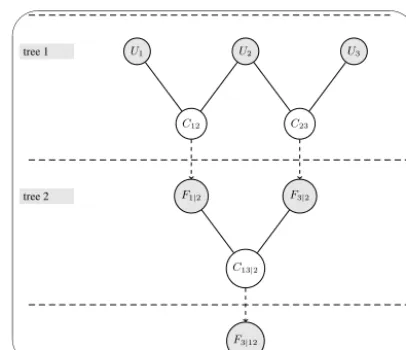
Figure 1. Hierarchical nesting of bivariate copulas in the

construc-tion of a 3-dimensional vine copula through condiconstruc-tional mixtures.

The joint cumulative distribution functionF1234is then ob-tained by integration, similarly as in Eq. (7):

F1234(x1, x2, x3, x4)=

x2 Z

−∞

x3 Z

−∞

C14|23(F1|23(x1|s, t ),

F4|23(x4|s, t ))dF23(s, t ). (12) Herein, the derivative of the bivariate CDFF23(x2, x3)is ex-pressed as dF23(x2, x3)=f23(x2, x3)dx2dx3. The functions

F1|23(x1|x2, x3) and F4|23(x4|x2, x3) are conditional CDFs (or CCDFs), and can also be expressed in terms of copulas:

F1|23(x1|x2, x3)=

∂C12|3(F1|3(x1|x3), F2|3(x2|x3))

∂F2|3(x2|x3)

F4|23(x4|x2, x3)=

∂C24|3(F2|3(x2|x3), F4|3(x4|x3))

∂F2|3(x2|x3)

(13)

where the CCDFs F1|3,F2|3 and F4|3 are calculated as in Eq. (8).

2.2 Fitting a 3- or 4-dimensional vine copula

Figures 1 and 2 illustrate the principle of constructing a 3-respectively 4-dimensional vine copula. Consider tree 1 in Figs. 1 and 2 where three (respectively four) uniform (on [0,1]) random variablesU1,U2 andU3 (orU1,U2,U3and

U4) are given and their pairwise dependences are described by the bivariate copulasC12andC23 (respectivelyC12,C23 and C34). Given a specific value of the second variable, these bivariate copulas can be conditioned (cf. dashed ar-rows in Figs. 1 and 2) through partial differentiation (Aas et al., 2009), resulting in the CCDFsF1|2andF3|2 (respec-tively F1|2,F3|2,F2|3andF4|3). The pairwise dependences between these CCDFs are then captured by the bivariate cop-ulaC13|2(respectively the copulasC13|2andC24|3). See tree

✬

✫

✩

✪

U1 U2 U3 U4

C12 C23 C34

F1|2 F3|2 F2|3 F4|3

C13|2 C24|3

F1|23 F4|23

C14|23

F4|123

tree 1

tree 2

tree 3

Figure 2. Hierarchical nesting of bivariate copulas in the

construc-tion of a 4-dimensional vine copula through condiconstruc-tional mixtures.

2 in Figs. 1 and 2. These latter copulas can then also be condi-tioned by partial differentiation to obtainF3|12(respectively

F3|12andF4|23). For the 4-dimensional vine copula, another bivariate copulaC14|23captures the pairwise dependence be-tween these CCDFs and can on its turn be partially differen-tiated to obtainF4|123. See tree 3 in Figure 2. The conditional CDFsF3|12andF4|123(of the 3- and 4-dimensional vine cop-ula, respectively) will be of use for simulation purposes (Aas et al., 2009). It should be noted that the hierarchical nesting of bivariate (conditional) copulas as presented here is just one of the possibilities and corresponds to what is called a D-vine (Aas et al., 2009).

In practice, the bivariate copulas in a higher tree of the vine copula (e.g.C13|2) are fitted as follows. Consider a set ofn data points, for all triplets(u1,i, u2,i, u3,i)(or for all

quadru-plets (u1,i, u2,i, u3,i, u4,i)), i=1, . . ., n, the CCDF values

(e.g. the CDF values according toF1|2andF3|2in the case of C13|2) are calculated. The bivariate copulas (e.g. C13|2) are then fitted to these “conditioned observations”, which are again approximately uniformly distributed onI.

2.3 Generating samples out of the vine copula

are uniformly distributed on_I, the 1-dimensional CCDF is highly important and is defined as (De Michele et al., 2007)

Gk|1...k−1(uk|u1, . . ., uk−1)

=_P(Uk≤uk|U1=u1, . . ., Uk−1=uk−1)

=

∂k−1

∂u1...∂uk−1C1...k(u1, . . ., uk)

∂k−1

∂u1...∂uk−1C1...k−1(u1, . . ., uk−1)

. (14)

Herein, the numerator is the mixed partial derivative of the

k-dimensional copula with respect to the conditioning vari-ables. The denominator is the copula density of the(k−1) -dimensional copula of the conditioning variables. In order to simulate a random sample out of the 3-D (respectively 4-D) conditional mixture copula, a random sample (t1, t2, t3) (or t1, t2, t3, t4) should be first generated from (T1, T2, T3) (respectivelyT1, T2, T3, T4) which are uniformly distributed random variables onI, and serve as random probability

lev-els of the CCDFs in the simulation algorithm which is listed next (of course for generating a 3-dimensional sample, step 4 should not be performed):

1. u1=t1;

2. u2=G₂−|11(t2|u1) ,where

G2|1(u2|u1)=

∂ ∂u1

C12(u1, u2); (15)

3. u3=G−3|121 (t3|u1, u2) ,where

G3|12(u3|u1, u2)=

∂2

∂u1∂u2C123(u1, u2, u3)

∂2

∂u1∂u2C12(u1, u2)

; (16)

4. u4=G−₄|1123(t4|u1, u2, u3) ,where

G4|123(u4|u1, u2, u3)

=

∂3

∂u1∂u2∂u3C1234(u1, u2, u3, u4)

∂3

∂u1∂u2∂u3C123(u1, u2, u3)

. (17)

The calculation of some partial derivatives, necessary for ob-taining the CCDFG4|123is given below:

∂3 ∂u1∂u2∂u3

C1234(u1, u2, u3, u4)

= ∂

∂u1

C14|23(G1|23(u1|u2, u3), G4|23(u4|u2, u3)), (18) with

G1|23(u1|u2, u3)=

∂2

∂u2∂u3C123(u1, u2, u3)

∂2

∂u2∂u3C23(u2, u3) =

∂ ∂u3C13|2

∂

∂u2C12(u1, u2),

∂

∂u2C23(u2, u3)

∂2

∂u2∂u3C23(u2, u3)

, (19)

and

G4|23(u4|u2, u3)=

∂2

∂u2∂u3C234(u2, u3, u4)

∂2

∂u2∂u3C23(u2, u3) =

∂ ∂u3C24|3

∂

∂u3C23(u2, u3),

∂

∂u3C34(u3, u4)

∂2

∂u2∂u3C23(u2, u3)

. (20)

Onceu1,u2,u3andu4are simulated, the corresponding val-ues ofx1,x2,x3andx4can be calculated by means of the in-verse marginal CDFsF₁−1,F₂−1,F₃−1andF₄−1, respectively.

3 Historical time series characteristics

Table 1. Observed probability ofpd=0 for the storms in the dif-ferent seasons

Probability ofpd=0 Winter 8.75 % Spring 11.21 % Summer 13.13 % Autumn 12.14 %

within the stormpd. It was observed that events with iden-tical values of variables occur in the observed time series. As this is not desirable for a copula-based analysis, in which ranks are important, random noise, uniformly distributed be-tween−0.1and+0.1 mm was introduced to all strictly posi-tive 10 min observations as described and motivated in Van-denberghe et al. (2010b). The choice of 0.1 mm was based on the pluviograph’s resolution. We also refer to Vandenberghe et al. (2010b) for a profound analysis of the dependences between the variables W, V, and D. Vandenberghe et al. (2010b) asserted that the hypothesis of stationarity of storms on the Uccle time series is fulfilled through seasonally sub-dividing the storms allowing copulas to be fitted per season. Therefore, the storm characteristics of the 105-year 10 min rainfall time series are subdivided according to the season in which the storms occurred. To this end, similarly as in Van-denberghe et al. (2010b), winter is defined as the months De-cember, January and February, spring as the months March, April and May, summer as the months June, July and August and autumn as the months September, October and Novem-ber. It was furthermore noticed that some of the storms have no internal dry 10 m intervals, i.e.pd=0. The set of storms within each season is then further subdivided into a subset of storms for whichpd=0 and a subset of storms for which

pd6=0. The observed probability ofpd=0 for the different seasons is listed in Table 1.

A kernel-smoothed distribution function was fitted to the observed values ofW,V,Dandpdas none of the commonly used probability distributions fitted the data well. AsDhas a theoretical minimum of 24 h, due to the selection criterion, the distribution was fit to D−24 h values, and afterwards, 24 h were added.

As the storm characteristicsV,WandDdo not reveal any information on the internal storm structure, andpdonly gives partial information, Huff curves, as derived in Vandenberghe et al. (2010a), are employed to provide statistical informa-tion on the internal structure. The idea to use Huff curves to generate an internal storm structure has also been adopted by Candela et al. (2014). Given the 105-year time series at hand, empirical Huff curves can be obtained by partitioning each storm in the time series in e.g. 20 identical time intervals at every 5 % of the total storm duration. Furthermore, storms were classified into seasons, and quartile groups according

0 10 20 30 40 50 60 70 80 90 100

0 10 20 30 40 50 60 70 80 90 100

percentage of storm duration

percentage of storm depth

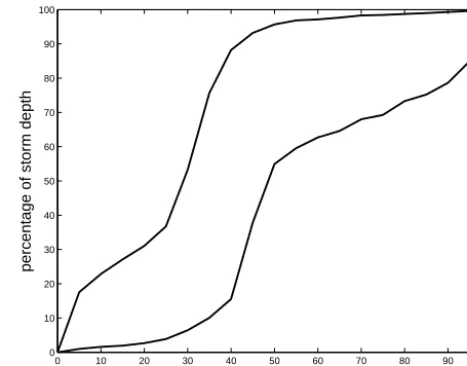
Figure 3. Huff curves for the second-quartile autumn storms. The

10 % (lower) and 90 % (upper) percentile curves are given.

to the quarter of the storm duration that received the largest amount of rainfall. For each season and each quartile group the corresponding Huff curves were obtained by visualizing the 10 and 90 % percentiles of the distribution. In this way, 16 Huff curves were obtained (four quartile groups per season). As an example, Fig. 3 illustrates the 10 and 90 % percentile curves of the second-quartile autumn storms. Vandenberghe et al. (2010a) showed that these curves are independent of the extremity of the storm.

4 Description of the rainfall model

4.1 The vine copula submodel: construction and use of vine copulas in the generation of a time series By examining the storm characteristics of the historical time series, it is observed that some storms have internal dry 10 min intervals while others have not. It was decided to fit, for each season, a 4-dimensional vine copula to the values ofW,V,Dand the non-zero values ofpd. Furthermore, for each season, a 3-dimensional vine copula was fitted to the values ofW,V andDin the casepd=0. In this way, depen-dences between the variables forpd=0 andpd6=0 are taken into account and four 3-dimensional and four 4-dimensional vine copulas are obtained.

0.1 0.1 0.2 0.2 0.3 0.3 0.4 0.4 0.5 0.6 0.7 0.8 0.9

0 0.2 0.4 0.6 0.8 1

0 0.2 0.4 0.6 0.8 1 0.1 0.1 0.2 0.2 0.3 0.3 0.4 0.5 0.6 0.7 0.8

0 0.2 0.4 0.6 0.8 1

0 0.2 0.4 0.6 0.8 1 0.1 0.1 0.2 0.2 0.3 0.3 0.4 0.5 0.6 0.7 0.8

0 0.2 0.4 0.6 0.8 1

0 0.2 0.4 0.6 0.8 1

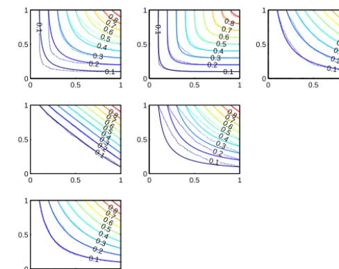
Figure 4. Contour plots of the empirical (dotted lines) and the

fitted Frank copulas (solid lines) for the different trees in the 3-dimensional vine copula for season 1. Bivariate copulas between W andV andV andD (top panel) and betweenW|V andD|V (bottom panel) are shown.

different copula families could be used to describe the de-pendences between the different variables (see Vandenberghe et al., 2010b). Yet, in this conceptual study, we opted to re-strict to the Frank copula family to describe the (conditional) bivariate dependences within the vine copulas, because of its ability to represent positive or negative dependence. Further-more, this family is frequently applied to describe bivariate hydrological phenomena (Pan et al., 2013). Alternative fami-lies could better fit the different dependences within the vine copula – however, the search for the best fitting copula was out of the scope of the current study. It should be remarked that two different ways of parametrizing the Frank copula exist. In this paper, the one that has the dependence parame-ter range of[−∞,+∞]is employed. The parameters of the Frank copulas are numerically estimated using the relation-ship between Kendall’s tau and the parameter value of the Frank copula (Genest, 1987):

τK=1−

4

θ 

1−

1 θ θ Z 0 t et₋₁dt



. (21)

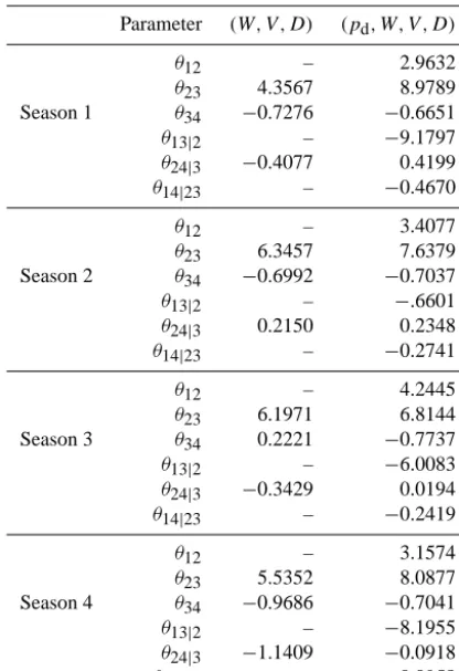
The fitted Frank copula parameters are presented in Table 3. Figures 4 and 5 show the contours of the Frank copulas and the empirical copulas for the 3- and 4-dimensional vine cop-ula for the first season. It can be seen that the Frank copcop-ula fits the empirical copulas fairly well. Only the dependence betweenW andV in the 3-dimensional vine copula and the dependence betweenpdandW, andW|V andD|V in the 4-dimensional vine copula are less well represented. In or-der to check whether the vine copulas preserve the depen-dence between the variables, two samples, with size 10 000,

0.1 0.1 0.2 0.3 0.4 0.5 0.60.7 0.8

0 0.5 1

0 0.5 1 0.1 0.1 0.20.3 0.40.5 0.6 0.7 0.8

0 0.5 1

0 0.5 1 0.1 0.2 0.3 0.4 0.50.6 0.70.8

0 0.5 1

0 0.5 1 0.10.2 0.30.4 0.50.6 0.70.8

0 0.5 1

0 0.5 1 0.1 0.2 0.3 0.40.5 0.60.7 0.8

0 0.5 1

0 0.5 1 0.1 0.2 0.3 0.4 0.50.6 0.70.8

0 0.5 1

0 0.5 1

Figure 5. Contour plots of the empirical (dotted lines) and the

fitted Frank copulas (solid lines) for the different trees in the 4-dimensional vine copula for season 1. Bivariate copulas between pdandW,WandV, andV andD(top panel), betweenpd|Wand

V|W, andW|V andD|V (middle panel) and betweenpd|W V and

D|W V (bottom panel) are shown.

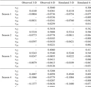
are simulated using the 3- and 4-dimensional vine copulas, respectively, based on the method described in Sect. 2.3. Ta-ble 2 shows the good correspondence between the observed and simulated pairwise dependences. To be able to transform samples from the fitted copula to real samples, the (inverse) marginal cumulative distribution functions ofpd,W,V and

Dare employed.

The inverse CDFs are then used to transform simulated uniformly distributed values in_I to values in_R. Once the simulated values of the quadruplet(pd, W, V , D)are known, a time series of 105 years of rectangular rainfall pulses with durationW and heightI=V /W, being separated by a dry durationD, is obtained. Of course, these rectangular pulses only correspond to the external storm structure. At this stage, only the timing of the beginning and the end of a storm is important. The pulse itself, characterized byW,V andpd, needs to be further disaggregated into finer-scale rainfall, which is elaborated upon in the next section.

4.2 The intrastorm-generating submodel:

disaggregation of rectangular pulses by means of Huff curves

Table 2. Correspondence between the observed and simulated pairwise dependences among(pd, W, V , D), expressed as Kendall’s tauτK.

Observed 3-D Observed 4-D Simulated 3-D Simulated 4-D

τ12 – 0.3040 – 0.3066

τ23 0.4140 0.6361 0.4118 0.6305 Season 1 τ34 −0.0804 −0.0736 −0.0754 −0.0790

τ13 – −0.0336 – −0.0092

τ24 −0.0831 −0.0341 −0.0760 −0.0425

τ14 – 0.0259 – 0.0111

τ12 – 0.3418 – 0.3423

τ23 0.5318 0.5888 0.5314 0.5866 Season 2 τ34 −0.0773 −0.0778 −0.0811 −0.0649

τ13 – −0.0183 – −0.0018

τ24 −0.0397 −0.0410 −0.0421 −0.0416

τ14 – 0.0221 – 0.0026

τ12 – 0.4060 – 0.4132

τ23 0.5243 0.5540 0.5248 0.5483 Season 3 τ34 0.0247 −0.0855 0.0222 −0.0820

τ13 – 0.0411 – 0.0602

τ24 −0.0079 −0.0613 −0.0109 −0.0672

τ14 – −0.0126 – −0.0332

τ12 – 0.3208 – 0.3276

τ23 0.4887 0.6058 0.4948 0.6016 Season 4 τ34 −0.1066 −0.0779 −0.1084 −0.0816

τ13 – −0.0287 – −0.0080

τ24 −0.1377 −0.0636 −0.1680 −0.0737

τ14 – −0.0086 – −0.0099

simulated storm pulses. Next, as the season and the quartile group are known, a random internal storm structure can be assigned to each simulated storm pulse on the basis of the corresponding 10 and 90 % Huff curves. To this end, time in-stants corresponding to the end of each 10 min interval within the storm are selected. The 10 and 90 % curves are then in-terpolated such that the values of the normalized cumulative storm depth for each of these time instants (expressed as a percentage of the total storm duration) are obtained.

The internal storm structure is then generated as follows. Firstly, time intervals having zero rainfall are randomly as-signed within the storm such that the sampled value of pd is respected. It should be noted that the first and the last in-terval of the storm cannot have zero rainfall in order to pre-serve the duration W of the storm. Furthermore, when the value ofpdis such that the storm should only contain one wet 10 min interval (i.e.pd is close to 1), the rainfall depth is evenly divided among the first and last 10 min intervals. In addition, the total length of a dry spell within a storm is con-strained to 23 h, i.e. 1 hour less than the selection criterion, in order to avoid that one storm would result in two differ-ent storms when the same storm selection criterion is applied on the simulated rainfall series. It should also be mentioned that storms that have a duration smaller than 40 min and for whichpd6=0, are disregarded in the generation of the

rain-fall series, because of the inability to assure the generation of the imposed quartile storm.

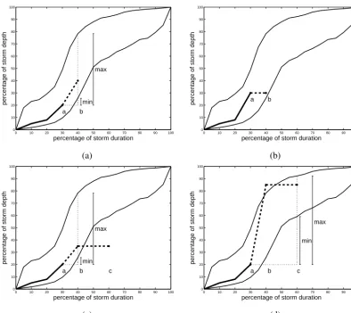
Secondly, the cumulative storm depths are randomly se-lected. This procedure calculates the normalized cumulative depth at the end of a time interval, i.e. at time instantb, be-fore moving to the next time interval. During the generation of the internal storm structure, three cases may occur, requir-ing different samplrequir-ing strategies. These cases are:

1. Time instantb is situated in between two consecutive wet 10 min intervals. In this case, a cumulative storm depth is randomly selected between the 10 and the 90 % percentile curves, ensuring that the cumulative storm depths do not decrease in time. Figure 6a illustrates this instant, where time instanta denotes the previous time instant at which a valueDnc(a)was selected, with

Dncthe normalized cumulative storm depth. The current time instantb, at which a valueDnc(b)is to be selected, is also indicated.Dnc(b)is randomly selected between a minimal (H10(b)) and a maximal value (H90(b)), indi-cated in the figure.H10(b), respectivelyH90(b), denote the value of the 10 %, respectively 90 % Huff curve, at instantb.

Table 3. Parameters of the bivariate Frank copulas in the

construc-tion of the 3- and 4-dimensional vine copulas.

Parameter (W, V , D) (pd, W, V , D)

θ12 – 2.9632

θ23 4.3567 8.9789 Season 1 θ34 −0.7276 −0.6651

θ13|2 – −9.1797

θ24|3 −0.4077 0.4199

θ14|23 – −0.4670

θ12 – 3.4077

θ23 6.3457 7.6379 Season 2 θ34 −0.6992 −0.7037

θ13|2 – −.6601

θ24|3 0.2150 0.2348

θ14|23 – −0.2741

θ12 – 4.2445

θ23 6.1971 6.8144 Season 3 θ34 0.2221 −0.7737

θ13|2 – −6.0083

θ24|3 −0.3429 0.0194

θ14|23 – −0.2419

θ12 – 3.1574

θ23 5.5352 8.0877 Season 4 θ34 −0.9686 −0.7041

θ13|2 – −8.1955

θ24|3 −1.1409 −0.0918

θ14|23 – −0.0958

performed (as the time interval betweenaandbshould be dry), and thus the cumulative storm depth takes the value of the previous time instant, i.e.Dnc(b)=Dnc(a), where Dnc(b) may be situated outside the percentile curves.

3. Time instant b corresponds to the end of a wet pe-riod. In this third case, depicted in Fig. 6c and d, the dry period starts at time instant band ends at time in-stant c. Two sampling strategies are possible, among which is chosen with equal probability. It is allowed that a cumulative storm depth is sampled according to the 10 and 90 % Huff curves either at time instant b

or at time instant c. When the first strategy is cho-sen (see Fig. 6c),Dnc(b)is sampled from the interval [max(Dnc(a), H10(b)), H90(b)], and the sampled value can hence be smaller thanH10(c), which indicates that the generated Huff curve will intersect the 10 % Huff curve, before reaching time instantcand will hence not remain between the 10 and 90 % boundaries. When the second strategy is chosen (see Fig. 6d),Dnc(b)is drawn from[max(Dnc(a), H10(c)), H90(c)], i.e. the sample is chosen according to the 10 and 90 % Huff curves at time instant c. The sampled value can hence be larger than H90(b), which indicates that the generated Huff

Table 4. Probability of a storm to belong to a certain quartile group.

Quartile group Probability [–]

First 0.3930

Second 0.2063

Third 0.1826

Fourth 0.2181

curve will intersect the 90 % Huff curve before reaching time instantb. Such flexibility is required as the fraction of dry spells often does not allow the curve to remain be-tween the 10 and 90 % boundaries. However, this flex-ibility is not a major problem, as at each time interval within the storm there are always 20 % of the historical relative cumulative storm depths outside these bound-aries by definition.

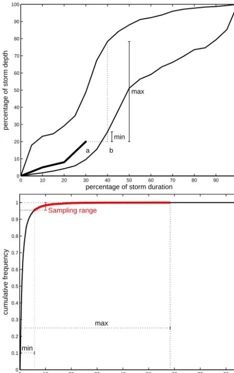
Based on the historical time series, it was observed that the increment in cumulative storm depth between two sub-sequent time instants in a Huff curve is not uniformly dis-tributed (this observation was neglected in Vandenberghe et al., 2010a). Smaller increments occur more often than large increments. This behaviour is simulated by first estab-lishing a cumulative probability distribution of strictly posi-tive increments on the basis of the 105-year time series. To this end, for all storms in a particular season and quartile group, the frequencies of normalized (strictly positive) in-crements of cumulative rainfall depths between two subse-quent wet periods were recorded. This empirical cumulative distribution function for the respective season and quartile group is then used to randomly select a normalized increase in storm depth for the subsequent wet time interval. Figure 7 illustrates the use of the cumulative distribution in the sam-pling procedure. In this figure, the minimum and maximum bounds of the increments are first determined on the basis of the Huff curves, as explained above. These bounds are then transferred to the cumulative distribution of normalized in-crements between which a value is randomly selected by uni-formly sampling within this sampling range (see Fig. 7). The corresponding difference percentage of total storm depth is then obtained.

5 Results

0 10 20 30 40 50 60 70 80 90 100 0

10 20 30 40 50 60 70 80 90 100

percentage of storm duration

percentage of storm depth

a b

min max

0 10 20 30 40 50 60 70 80 90 100

0 10 20 30 40 50 60 70 80 90 100

percentage of storm duration

percentage of storm depth a b

(a) (b)

0 10 20 30 40 50 60 70 80 90 100

0 10 20 30 40 50 60 70 80 90 100

percentage of storm duration

percentage of storm depth

a b

min max

c

0 10 20 30 40 50 60 70 80 90 100

0 10 20 30 40 50 60 70 80 90 100

percentage of storm duration

percentage of storm depth

a b c

min max

(c) (d)

Figure 6. Illustration of the generation of an internal storm structure. The part of the Huff curve that is already generated (up to time

instant a) is indicated by a thick solid line. The value at time instant b needs to be determined. Four sampling strategies are possible: sampling in between two consecutive wet periods (case 1; a), sampling at the end of a dry period (case 2; b), sampling at the end of a wet period followed by a dry period with a selection on the basis of the current time instant (case 3; c) and with a selection on the basis of the last time instant in the dry period (case 3; d).

model performs well in the reproduction of aggregated rain-fall statistics, the 100 time series are furthermore regarded as equally probable realizations and the statistics are calcu-lated on a yearly basis. The traditional first- and second-order statistical moments (i.e. mean and variance), autocorrelation (AC) at different time lags and the zero depth probability (ZDP) are calculated along with the third-order central mo-ment (skewness). These statistics are calculated on a yearly basis for each ensemble member at aggregation levels of 1/6, 1, 3, 6, 12 and 24 h. Thus, for an aggregation level, 100×105 values of each of these statistics are obtained, such that a bun-dle of 100 empirical cumulative distributions can be estab-lished, i.e. one distribution per ensemble member. The em-pirical cumulative distribution of the values of the statistics of the observed time series can then be compared with this bundle. If the empirical CDF of the observed statistics is situ-ated within the bundle of distributions obtained by the model, the model performs well.

0 10 20 30 40 50 60 70 80 90 100 0

10 20 30 40 50 60 70 80 90 100

percentage of storm duration

percentage of storm depth

a b

min max

0 10 20 30 40 50 60 70 80

0 0.1 0.2 0.3 0.4 0.5 0.6 0.7 0.8 0.9 1

difference % of total storm depth

cumulative frequency

Sampling range

min

max

Figure 7. Illustration of the procedure to sample the storm depth at

the next time instant (b). First, the minimal and maximal increment in percentage of storm depth at time instant b are determined (top panel). Then, the corresponding sampling range in the CDF of nor-malized increments is defined based on the minimal and maximal increment in percentage of storm depth derived from the top panel (bottom panel).

for a 24 h aggregation level), is probably due to the selection of the dry periods within the storm. For storms that have a duration of more than 1 hour, these zero intervals are prob-ably not connected as no temporal correlation is taken into account during the selection of dry periods, such that fewer dry periods are obtained after the aggregation than what is observed in the Uccle time series. Future research will fur-ther elaborate on a better selection of dry periods within the storm.

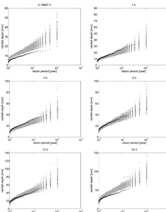
As simulated time series are often used to simulate ex-treme discharges (Verhoest et al., 2010), the behaviour of the modelled extreme rainfall was also assessed. Figure 9 shows the annual maximum rainfall depths of the ensem-ble and of the observed rainfall series related to empirical

0 0.01 0.02 0.03

0 0.5

1 Mean

0 0.05 0.1

0 0.5

1 Variance

0 0.01 0.02 0.03

0 0.5

1 Lag-1 autocovariance

0 0.005 0.01 0.015 0.02

0 0.5

1 Lag-2 autocovariance

0.850 0.9 0.95 1

0.5

1 Zero depth probability

0 1 2 3 4

0 0.5

1 3rd central moment

(a)

0 0.05 0.1 0.15 0.2

0 0.5

1 Mean

0 0.5 1 1.5

0 0.5

1 Variance

0 0.1 0.2 0.3 0.4

0 0.5

1 Lag-1 autocovariance

0 0.1 0.2 0.3 0.4

0 0.5

1 Lag-2 autocovariance

0.7 0.8 0.9 1

0 0.5

1 Zero depth probability

0 20 40 60 80

0 0.5

1 3rd central moment

(b)

Figure 8. Comparison of the empirical cumulative distributions of

the yearly statistics of the observed time series (black line) and the bundle of empirical cumulative distributions of synthetic time series generated by means of the copula-based model (grey) at a 10 min (a) and a 1 h aggregation level (b).

Figure 9. Comparison of empirically derived annual maxima related to the empirical return periods for different aggregation levels on the

observed (black asterisks) and ensemble of synthetic time series generated by means of the copula-based rainfall model (grey asterisks).

6 Conclusions

This study is the first in its kind in which a continuous stochastic rainfall generator is developed that uses vine cop-ulas to describe the storms and their arrival process. The in-ternal storm structure is based on the concept of Huff curves, while the fraction of dry periods within the storm is deter-mined by the copulas. The main advantage of this approach is that the model is completely data driven and is easier to calibrate than other rainfall generators such as the commonly used Modified Bartlett–Lewis model as, once the structure of the vine copula is determined, the calibration is reduced to estimating the parameters of the bivariate copulas. It should, however, be noted that we have at our disposal an

exception-ally long time series of rainfall data on the basis of which the vine copulas are determined. If one would follow the same approach and search for the best-fitting copula family on a more commonly shorter time series of e.g.<50 years of rain-fall data, one could be faced with difficulties as the number of storms per season may become too small for fitting the copulas.

depen-dence between these storm characteristics and the dry frac-tion within the storm. These vine copulas were fitted to the observed storm characteristics of a 105-year time series of 10 min rainfall. Because of its frequent successful applica-tion in hydrological applicaapplica-tions, the Frank copula family was chosen to be used within the vine copulas. On the ba-sis of these vine copulas, values of these four storm charac-teristics were drawn, representing the external storm struc-ture, ensuring a time series of 105 years of rectangular rain-fall pulses. According to their seasonal probability of occur-rence, storms with zero dry fractions were sampled from the 3-dimensional vine copulas. The internal storm structure of the rectangular pulses is superimposed based on Huff curves, which were identified on the basis of the observed time se-ries, leading to the generation of continuous 10 min rainfall time series. In the generation of the internal storm structure, it is ensured that the fraction of dry periods within the storm as drawn from the vine copulas, is maintained. The internal storm structures are furthermore generated according to the probability of occurrence of the quartile storms in the ob-served time series, and the season in which they occur. In or-der to determine the difference of cumulative storm depths in the internal storm structure, the empirical cumulative PDF of increments between two subsequent wet periods in the storm is employed. In this way it is guaranteed that smaller incre-ments occur more often than larger increincre-ments, as was ob-served in the measured time series.

In order to evaluate the performance of the rainfall model, an ensemble of 100 time series of ca. 105-year 10 min rainfall was generated, such that stochastic effects were accounted for. The results show that the copula-based rainfall model represents the mean value of the time series well, whereas the other statistics are either represented (fairly) well, over-or underestimated, depending on the aggregation level. A second evaluation of the generated ensemble encompassed the calculation of the annual maximum series, for different aggregation levels. It was observed that the annual maxima simulated by means of the copula-based model were larger than the observed maxima for an aggregation level of 10 min, and the moderate return period of the 24 h aggregation level. For aggregation levels of 1–12 h and the smaller and larger return periods of an aggregation level of 24 h, a good cor-respondence between the simulated and observed extremes was observed. Future research will reveal whether the rep-resentation of the ZDP statistic for larger aggregation levels by the copula-based model can be improved by better select-ing the internal dry storm periods. The performance of the copula-based model will also be compared to state-of-the-art stochastic rainfall generators. Also, it should be inves-tigated whether including other bivariate copula families in the vine copulas can further improve the performance of the vine-copula-based model.

Acknowledgements. This research has been performed in the framework of projects G.0837.10 and G.0013.11 granted by the Research Foundation Flanders.

Edited by: C. De Michele

References

Aas, K. and Berg, D.: Models for construction of multivariate de-pendence - a comparison study, Eur. J. Financ., 15, 639–659, 2009.

Aas, K., Czado, C., Frigessi, A., and Bakken, H.: Pair-copula con-structions of multiple dependence, Insurance: Mathematics and Economics, 44, 182–198, 2009.

Bedford, T. and Cooke, R.: Probability density decomposition for conditionally dependent random variables modeled by vines, Ann. Math. Artif. Intel., 32, 245–268, 2001.

Bedford, T. and Cooke, R.: Vines – A new graphical model for de-pendent random variables, Ann. Stat., 30, 1031–1068, 2002. Bonta, J. and Rao, A.: Factors affecting the identification of

inde-pendent storm events, J. Hydrol., 98, 275–293, 1988.

Candela, A., Brigandì, G., and Aronica, G. T.: Estimation of syn-thetic flood design hydrographs using a distributed rainfall-runoff model coupled with a copula-based single storm rain-fall generator, Nat. Hazards Earth Syst. Sci., 14, 1819–1833, doi:10.5194/nhess-14-1819-2014, 2014.

Chow, V., Maidment, D., and Mays, L.: Applied Hydrology, McGraw-Hill Book Company, New York, 588 pp., 1988. De Jongh, I., Verhoest, N. E. C., and De Troch, F.: Analysis of a

105-year time series of precipitation observed at Uccle, Belgium, Internat. J. Climatol., 26, 2023–2039, 2006.

De Michele, C. and Salvadori, G.: A generalized Pareto intensity-duration model of storm rainfall exploiting 2-copulas, J. Geo-phys. Res., 108, D24067, 2003.

De Michele, C., Salvadori, G., Canossi, M., Petaccia, A., and Rosso, R.: Bivariate statistical approach to check adequacy of dam spill-way, J. Hydrol. Eng., 10, 50–57, 2005.

De Michele, C., Salvadori, G., Passoni, G., and Vezzoli, R.: A multi-variate model of sea storms using copulas, Coast. Eng., 54, 734– 751, 2007.

Demarée, G.: The centennial recording raingauge of the Uccle Plateau: Its history, its data and its applications, La Houille Blanche – Revue International de l’Eau, 4, 95–102, 2003. Evin, G. and Favre, A.-C.: A new rainfall model based on the

Neyman-Scott process using cubic copulas, Water Resour. Res., 44, W03433, doi:10.1029/2007WR006054, 2008.

Evin, G. and Favre, A.-C.: Further developments of a transient Poisson-cluster model for rainfall, Stoch. Env. Res. Risk A., 27, 831–847, 2013.

Favre, A., Adlouni, S. E., Perreault, L., Thiemonge, N., and Bobee, B.: Multivariate hydrological frequency analysis using copulas, Water Resour. Res., 40, W01101, doi:10.1029/2003WR002456, 2004.

Ganguli, P. and Reddy, M.: Probabilistic assessment of flood risks using trivariate copulas, Theor. Appl. Climatol., 111, 341–360, 2013.

Genest, C., Favre, A., Beliveau, J., and Jacques, C.: Metael-liptical copulas and their use in frequency analysis of mul-tivariate hydrological data, Water Resour. Res., 43, W09401, doi:10.1029/2006WR005275, 2007.

Gräler, B.: Modelling skewed spatial random fields through the spa-tial vine copula, Spaspa-tial Statistics, 10, 87–102, 2014.

Gräler, B., van den Berg, M. J., Vandenberghe, S., Petroselli, A., Grimaldi, S., De Baets, B., and Verhoest, N. E. C.: Multi-variate return periods in hydrology: a critical and practical re-view focusing on synthetic design hydrograph estimation, Hy-drol. Earth Syst. Sci., 17, 1281–1296, doi:10.5194/hess-17-1281-2013, 2013.

Grimaldi, S. and Serinaldi, F.: Design hyetograph analysis with 3-copula function, Hydrolog. Sci. J., 51, 223–238, 2006.

Gyasi-Agyei, Y.: Copula-based daily rainfall disaggregation model, Water Resour. Res., 47, W07535, doi:10.1029/2011WR010519, 2011.

Gyasi-Agyei, Y. and Melching, C.: Modelling the dependence and internal structure of storm evens for continuous rainfall simula-tion, J. Hydrol., 464, 249–261, 2012.

Hobæk Haff, I., Aas, K., and Frigessi, A.: On the simplified pair-copula construction – Simply useful or too simplistic?, J. Multi-variate Anal., 101, 1296–1310, 2010.

Huff, F.: Time distribution of rainfall in heavy storms, Water Resour. Res., 3, 1007–1019, 1967.

Joe, H.: Multivariate Models and Dependence Concepts, Chapman and Hall, 399 pp., 1997.

Kao, S. and Govindaraju, R.: Trivariate statistical analysis of ex-treme rainfall events via the Plackett family of copulas, Water Resour. Res., 44, W02415, doi:10.1029/2007WR006261, 2008. Katz, R. and Parlange, M.: Overdispersion phenomenon in

stochas-tic modeling of precipitation, J. Climate, 11, 591–601, 1998. Kavvas, M. and Delleur, J.: A stochastic cluster model of daily

rain-fall sequences, Water Resour. Res., 17, 1151–1160, 1981. Kurowicka, D. and Cooke, R.: Sampling algorithms for generating

joint uniform distributions using the vine-copula method, Com-put. Stat. Data An., 51, 2889–2906, 2007.

Ma, M., Song, S., Ren, L., Jiand, S., and Song, J.: Multivariate drought characteristics using trivariate Gaussian and Student t copulas, Hydrol. Process., 27, 1175–1190, 2013.

Menabde, M. and Sivapalan, M.: Modeling of rainfall time series and extremes using bounded random cascades and Levy-stable distributions, Water Resour. Res., 36, 3293–3300, 2000. Mendes, B. and Accioly, V.: Robust Pair-Copula based forecasts of

realized volatitiliy, Applied Stochastic Models in Business and Industry, 30, 183–199, 2014.

Nelsen, R.: An Introduction to Copulas, in: Lecture Notes in Statis-tics, edited by: Bickel, P., Diggle, P., Fienberg, S., Krickeberg, K., Olking, I., Wermuth, N., and Zeger, S., pp. 216, Springer-Verlag, New York, 2006.

Nikololoupoulos, A., Joe, H., and Li, H.: Vine coplas with asym-metric tail dependence and applications to financial return data, Computational Statistics and Data Analysis, 56, 3659–3673, 2012.

Ntegeka, V. and Willems, P.: Trends in multidecadal oscillations in rainfall extremes, based on a more than 100-year time series of 10 min rainfall intensities at Uccle, Belgium, Water Resour. Res., 44, W07402, doi:10.1029/2007WR006471, 2008.

Onof, C., Chandler, R., Kakou, A., Northrop, P., Wheater, H., and Isham, V.: Rainfall modelling using Poisson-cluster processes: a review of developments., Stoch. Env. Res. Risk A., 14, 384–411, 2000.

Pan, M., Yuan, X., and Wood, E. F.: A probabilistic view on drought recovery., Geophys. Res. Lett., 40, 3637–3642, 2013.

Pham, M. T., Vanhaute, W. J., Vandenberghe, S., De Baets, B., and Verhoest, N. E. C.: An assessment of the ability of Bartlett-Lewis type of rainfall models to reproduce drought statistics, Hy-drol. Earth Syst. Sci., 17, 5167–5183, doi:10.5194/hess-17-5167-2013, 2013.

Restrepo-Posada, P. and Eagleson, P.: Identification of independent rainstorms, J. Hydrol., 55, 303–319, 1982.

Rodriguez-Iturbe, I., Cox, D., and Isham, V.: Some models for rain-fall based on stochastic point processes, Proc. R. Soc. Lon. Ser.-A, 410, 269–288, 1987a.

Rodriguez-Iturbe, I., Febres de Power, B., and Valdés, J.: Rectangu-lar pulses point process models for rainfall: analysis of empirical data, . Geophys. Res., 92, 9645–9656, 1987b.

Salvadori, G. and De Michele, C.: Analytical calculation of storm volume statistics involving Pareto-like intensity-duration marginals, Geophys. Res. Lett., 31, L04502, doi:10.1029/2003GL018767, 2004.

Salvadori, G. and De Michele, C.: Statistical characterization of temporal structure of storms, Adv. Water Resour., 29, 827–842, 2006.

Salvadori, G. and De Michele, C.: On the use of copulas in hydrol-ogy: theory and practice, J. Hydrol. Eng., 12, 369–380, 2007. Serinaldi, F. and Grimaldi, S.: Fully nested 3-copula: procedure and

application on hydrological data, J. Hydrol. Eng., 12, 420–430, 2007.

Sklar, A.: Fonctions de répartition ándimensions et leurs marges., Publications de l’Institut de Statistique de l’Université de Paris, 8, 229–231, 1959.

Song, S. and Singh, V.: Meta-elliptical copulas for drought fre-quency analysis of periodic hydrologic data, Stoch. Env. Res. Risk A., 24, 425–444, 2010.

Vaes, G., Willems, P., and Berlamont, J.: 100 years of Belgian rain-fall: Are there trends?, Water Sci. Technol., 45, 55–61, 2002. Vandenberghe, S., Verhoest, N. E. C., Buyse, E., and De Baets,

B.: A stochastic design rainfall generator based on copulas and mass curves, Hydrol. Earth Syst. Sci., 14, 2429–2442, doi:10.5194/hess-14-2429-2010, 2010a.

Vandenberghe, S., Verhoest, N. E. C., and De Baets, B.: Fitting bi-variate copulas to the dependence structure between storm char-acteristics: A detailed analysis based on 105 year 10 min rainfall, Water Resour. Res., 46, W01512, doi:10.1029/2009WR007857, 2010b.

Vandenberghe, S., Verhoest, N. E. C., Onof, C., and De Baets, B.: A comparative copula-based bivariated frequency analysis of observed and simulated storm evens: a cast study on Bartlett-Lewis modeled rainfall, Water Resour. Resear., 47, W07529, doi:10.1029/2009WR008388, 2011.

Verhoest, N., Troch, P., and De Troch, F.: On the applicability of Bartlett-Lewis rectangular pulses models in the modeling of de-sign storms at a point, J. Hydrol., 202, 108–120, 1997.

Verhoest, N. E. C., Vandenberghe, S., Cabus, P., Onof, C., Meca-Figueras, T., and Jameleddine, S.: Are stochastic point rainfall models able to preserve extreme flood statistics?, Hydrol. Pro-cess., 24, 3439–2445, 2010.

Viglione, A., Castellarin, A., Rogger, M., Merz, R., and Blöschl, G.: Extreme rainstorms: Comparing regional envelope curves to stochastically generated events, Water Resour. Res., 48, W01509, doi:10.1029/2011WR010515, 2012.

Willems, P.: A spatial rainfall generator for small spatial scales, J. Hydrol., 252, 126–144, 2001.

Wong, G., Lambert, M., Leonard, M., and Metcalfe, A.: Drought Analysis using trivariate copulas conditional on climatic states, J. Hydrol. Eng., 15, 129–141, 2010.

Xiong, L., Yu, K., and Gottschalk, L.: Estimation of the distribution of annual runoff from climatic variables using copulas, Water Resour. Res., 50, 7134–7152, 2014.

Zhang, D.: Vine copulas and applications to the European Union sovereign debt analysis, International Review of Financial Anal-ysis, 36, 46–56, 2014.