Effects of LiDAR point density and landscape context on estimates
of urban forest biomass
Kunwar K. Singh
a,⇑, Gang Chen
b, James B. McCarter
a, Ross K. Meentemeyer
a aCenter for Geospatial Analytics, Department of Forestry and Environmental Resources, North Carolina State University, Raleigh, NC 27695, USA
b
Department of Geography and Earth Sciences, University of North Carolina, 9201 University City Blvd, Charlotte, NC 28223, USA
a r t i c l e
i n f o
Article history:
Received 3 October 2014
Received in revised form 13 December 2014 Accepted 19 December 2014
Available online 3 February 2015
Keywords:
LiDAR Biomass
Development density Canopy stratification Multiple linear regression Large-area assessment Point density
a b s t r a c t
Light Detection and Ranging (LiDAR) data is being increasingly used as an effective alternative to conven-tional optical remote sensing to accurately estimate aboveground forest biomass ranging from individual tree to stand levels. Recent advancements in LiDAR technology have resulted in higher point densities and improved data accuracies accompanied by challenges for procuring and processing voluminous LiDAR data for large-area assessments. Reducing point density lowers data acquisition costs and over-comes computational challenges for large-area forest assessments. However, how does lower point den-sity impact the accuracy of biomass estimation in forests containing a great level of anthropogenic disturbance? We evaluate the effects of LiDAR point density on the biomass estimation of remnant forests in the rapidly urbanizing region of Charlotte, North Carolina, USA. We used multiple linear regression to establish a statistical relationship between field-measured biomass and predictor variables derived from LiDAR data with varying densities. We compared the estimation accuracies between a general Urban For-est type and three ForFor-est Type models (evergreen, deciduous, and mixed) and quantified the degree to which landscape context influenced biomass estimation. The explained biomass variance of the Urban Forest model, usingadjusted R2, was consistent across the reduced point densities, with the highest dif-ference of 11.5% between the 100% and 1% point densities. The combined estimates of Forest Type bio-mass models outperformed the Urban Forest models at the representative point densities (100% and 40%). The Urban Forest biomass model with development density of 125 m radius produced the highest adjusted R2(0.83 and 0.82 at 100% and 40% LiDAR point densities, respectively) and the lowest RMSE val-ues, highlighting a distance impact of development on biomass estimation. Our evaluation suggests that reducing LiDAR point density is a viable solution to regional-scale forest assessment without compromis-ing the accuracy of biomass estimates, and these estimates can be further improved uscompromis-ing development density.
Ó2015 International Society for Photogrammetry and Remote Sensing, Inc. (ISPRS). Published by Elsevier B.V. All rights reserved.
1. Introduction
Loss of forest biomass in urbanizing regions is a growing con-cern worldwide (Seto et al., 2012). Changes in biomass impact critical ecological and environmental processes necessary for the maintenance of biodiversity and ecosystem health, often for the long-term and with slowed or no opportunity for recovery. Long-term impacts include changes in regional nitrogen and
car-bon storage and flux (Groffman et al., 2006; Magnani et al., 2007), increases in urban heat island effects (Imhoff et al., 2010), and increased concentration of atmospheric carbon dioxide
(Nowak and Greenfield, 2012), as well as changes in human
per-ceptions of environmental quality and well-being (Grove et al., 2006). As urban forests decrease in size and number, we face an ever-increasing need to quantify the remaining resources. However, some of the most vulnerable forests around growing U.S. cities are the least accessible for ecological measurement due to the high proportion of privately owned land typical of metropolitan landscapes (Meentemeyer et al., 2013). Since bio-mass directly relates to the tree structure – height and diameter at breast height – cost-effective regional-scale remote sensing data that characterize the structure of forest stands are needed to
http://dx.doi.org/10.1016/j.isprsjprs.2014.12.021
0924-2716/Ó2015 International Society for Photogrammetry and Remote Sensing, Inc. (ISPRS). Published by Elsevier B.V. All rights reserved.
⇑Corresponding author at: Department of Forestry and Environmental Resources, North Carolina State University, Raleigh, NC 27695, USA. Tel.: +1 704 359 7139; fax: +1 919 515 3439.
E-mail addresses: [email protected](K.K. Singh),[email protected] (G. Chen),[email protected](J.B. McCarter),[email protected](R.K. Meentemeyer).
Contents lists available atScienceDirect
ISPRS Journal of Photogrammetry and Remote Sensing
quantify biomass in urban landscapes. LiDAR provides structural data for forest analysis studies.
Airborne and terrestrial LiDAR has emerged as a key remote sensing technology for the accurate estimation of forest biomass ranging from individual tree to stand levels (Mascaro et al., 2011; Zolkos et al., 2013), and has been successfully applied to quantify and measure biomass of tropical forests (Drake et al., 2003), shrubs (Estornell et al., 2011), understory vegetation (Seidel et al., 2012), unmanaged Mediterranean forests (Garcia et al., 2010), and urban forests (He et al., 2013). However, these applications have not char-acterized forest types found along urban–rural gradients, rarely address the impact of landscape context on biomass estimation across the urbanizing landscapes, and lack large-area assessment, for example, an area comprised of a county (>1000 km2), or multi-ple counties. Recent advancements in LiDAR technology have resulted in improved data accuracies and higher point densities, which can greatly increase the costs (Renslow et al., 2000), and poses a challenge to a cost-effective procurement and processing of voluminous LiDAR data for large-area assessments. To overcome these challenges, large-area assessments are typically based on plot-level regression models either ‘alone’ (Drake et al., 2002) or through ‘fusion’ of sampled LiDAR transects with spectral data (Popescu et al., 2004). However, these approaches to large-area assessments are often not suitable for urban forest studies due to the presence of different forest types, and the high degree of heter-ogeneity at fine scales caused by repeated anthropogenic distur-bances, such as conversion of forests to development. Therefore, reducing LiDAR point density may provide a solution for cutting procurement costs and overcoming computational challenges for large-area assessments. The concept of reducing point density may also help analyze features in point clouds derived from auto-mated methods (e.g. Structure from Motion technique) designed to generate a 3D point cloud from video sequences filmed from new mobile sensors.
Data procurement and processing costs limit the extent to which LiDAR is useful for large-area studies. To achieve both cost-effective and accurate results, data acquisition parameters are optimized (Lovell et al., 2005; Naesset, 2009) while tradeoffs are made between point density and estimation accuracy
(Jakubowski et al., 2013; Magnusson et al., 2007; Zhao et al.,
2009). To date, studies considering the optimization of LiDAR point densities, such asGobakken and Naesset (2008), Lim et al. (2008), andTreitz et al. (2012), were mainly focused on natural environments and rarely accounted for the influence of landscape context (e.g., surrounding urban development or forest stratifica-tion following disturbance) on forest structure and biomass estimation.
Forest structural heterogeneity and factors modifying it, such as urbanization (McHale et al., 2009), are important determinants in biomass estimation. Studies documenting the effects of urbaniza-tion on forest structure have found lower stem densities in young stands, increased forest edge opening, and increased biomass growth compared to rural stands (Gregg et al., 2003; Moran, 1984; O’Brien et al., 2012). These structural variations affect the total biomass, while also potentially affecting the capacity to mea-sure biomass using LiDAR. Canopy stratification has been sug-gested to overcome potential estimation errors due to structural variation (Swatantran et al., 2011). Canopy stratification is a useful organizational tool for the study of the vertical distribution of plants and animals (Baker and Wilson, 2000), and is considered an index of vertical structure where the higher number of canopy strata represents increased complexity in the forest stands (Parker and Brown, 2000). Fundamental differences in the heterogeneity of forests types in urbanizing landscapes suggest the need for a broader perspective and innovative approaches for the use of LiDAR point density in forest biomass estimation.
In this study, we evaluate the effects of LiDAR point density on the estimation of aboveground biomass of remnant forests in the rapidly urbanizing region of Charlotte, North Carolina, USA. Using multiple linear regression (MLR), we established relationships between field-based biomass estimates and LiDAR-derived predic-tor variables (PVs) for a general urban forest type and three specific Forest Type biomass models, referred to as Urban Forest and Forest Types (coniferous, deciduous, and mixed). For the Urban Forest, we developed models using PVs of LiDAR data at eight point densities while for the Forest Type models we used the original LiDAR data and the point densities that produced similar biomass estimates for the Urban Forest. We then compared accuracies of the Urban Forest and Forest Type models in addition to comparison of top performing biomass models between the Urban Forest and a com-bined estimate for the Forest Type models. We quantified the degree to which the presence of built development (e.g., buildings, roads, and parking lots) influenced biomass estimation. Finally, we analyzed the effect of canopy stratification on biomass estimation for both the Urban Forest and Forest Type models.
2. Materials and methods
2.1. Study system
This study focuses on the urban remnant forests of Mecklen-burg County, North Carolina (Fig. 1a). The county is located within the Piedmont physiographic province in the center of the Charlotte Metropolitan Area and covers 1415 km2. The region’s topography is characterized by rolling flat lands with elevation ranging from 252 m in the northern part of the county to about 159 m in the south. Forested landscapes in the area are primarily comprised of oak–hickory–pine forests that have developed on former timber plantation sites as well as through natural regeneration on aban-doned farmland. In recent years, urban sprawl, with low- to med-ium-density housing, has converted forest and farmland dominated landscapes into an array of developed land cover types with highly fragmented and complex urban forests. According to the American Forests report in 2008, Mecklenburg County has experienced a 33% decline in its tree canopy between 1985 and 2008, and will suffer an additional loss of3% by the year 2015 under recent trends.
2.2. Field data
We conducted field measurements during the years 2010–2012 as part of the Charlotte ULTRA-Ex (Urban Long-Term Research Areas Exploratory) study designed to analyze socio-ecological interactions driving the persistence of private forest. Within each forest site, we established three to five 11.5 m fixed-radius random field plots (400 m2) (Fig. 1b). We measured the diameter at breast height (dbh) of all native and invasive woody plants greater than 5 cm, including vines. Other parameters measured in each plot include geographic coordinates, merchantable height, species’ name and type (deciduous vs. evergreen), and predominant land cover type. Prior to the analysis, we categorized all field plots into deciduous, coniferous, and mixed forest types using a threshold of 75% predominant land cover type. If a plot consisted of over 75% deciduous or coniferous trees, we labeled the plot as deciduous or coniferous, respectively. We labeled plots comprised of less than 75% deciduous or coniferous forest as mixed plots. To maintain the uniformity in modeling biomass across the forest types, we selected a similar number of field plots in each Forest Type result-ing in a collection of 70 plots comprised of 22 deciduous, 23 conif-erous, and 25 mixed plots.
2.3. LiDAR data
We used leaf-off multiple return LiDAR data acquired April 11– 14, 2012, and obtained from the Storm Water Services Division of Charlotte-Mecklenburg County government office. Original data acquisition was carried out by Pictometry International (Rochester, USA) using Optech’s ALTM Gemini 3100 LiDAR system with aver-age point spacing of 1 m between any two neighboring points over the study system (Godwin et al., 2015).
2.4. LiDAR data processing and reduced point densities
We clipped the original LiDAR tiles at the plot-level using 12 m radius to account for any possible misalignment due to GPS posi-tional errors. Then, we reduced the original LiDAR point density to 80%, 60%, 40%, 20%, 10%, 5%, and 1% densities (Fig. 2;Table 1) using the ‘percentage of the total points’ reduction algorithm developed at Boise Center Aerospace Laboratory, Boise, Idaho (BCAL LiDAR Tools, 2013). This algorithm reduces LAS files (LiDAR data format) by the percentage of the total points using random selection from the pool of equal height points in each return. We selected this data reduction approach over other approaches, such as point density or point spacing, based on two primary consider-ations: (1) the inconsistency of point spacing and point density throughout the LiDAR tiles and field plots, and (2) reduction by percentage offers nearly consistent sampling across the tiles for
large scale analysis (Anderson et al., 2006; Magnusson et al., 2007). This resulted in eight plot-level LiDAR datasets, including seven sets of reduced point densities.
2.5. Processing and extracting variables
2.5.1. Field-based aboveground biomass estimation
To identify an optimal LiDAR point density, we applied a gener-alized allometric equation (Eq. (1)) (Jenkins et al., 2003) to the tree species found in each field plot to estimate biomass for individual trees using field-baseddbhand parameters from the appropriate species group as documented inJenkins et al. (2003)and listed inTable 2.
bm¼Expðb0þb1lnðdbhÞÞ ð1Þ
where bm is total aboveground biomass (kg dry weight) for trees > 5 cm indbh,Expis the exponential function,dbhis the diam-eter at breast height in centimdiam-eters (cm), ln is the natural log basee (2.718282), andb0andb1are parameters for hardwood and soft-wood tree species groups (Table 2).
We aggregated tree species observed in the field into hardwood and softwood species groups. We used parameters of each respec-tive species group to calculate biomass for individual trees and then averaged the biomass at plot-level by applying a tons per hectare conversion unit. We useddbh to estimate biomass due to: (1)dbhis the most stable predictor for regression models com-pared to predictors that incorporate LiDAR-derived tree height and
crown diameter (Popescu, 2007), and (2) species-independent bio-mass equations only requiredbhcompared to species-dependent.
2.5.2. LiDAR metrics extraction
We extracted plot-level metrics from LiDAR data using FUSION software developed at Pacific Northwest Research Station, Seattle,
WA (McGaughey, 2014). We normalized the clipped plot-level
LiDAR datasets using 1 m resolution digital elevation model derived from LiDAR ground returns. This process removed topogra-phy effects from LiDAR points across the datasets for yielding
height-above-groundvalues. For extracting plot-level tree metrics, we used the height range 1.5–35 m to exclude understory vegeta-tion and objects taller than the trees found within the region. We calculated descriptive statistics for normalized LiDAR point densi-ties across the entire vertical profile (e.g., minimum, maximum, variance, interquartile distance, percentiles, etc.) and canopy related metrics (e.g., percentage of first returns above 3 m, percent-age of first return above mean, and mode, etc.) (Frazer et al., 2011; Jakubowski et al., 2013). We derived and further identified a total of 37 metrics from previous studies at the plot-level (Table 3).
Fig. 2.An illustration of percentage-based LiDAR data reduction. The total number of LiDAR points (TP) and average point spacing (PS) are shown for each point density reduction at plot-level (400 m2
).
Table 1
Distribution of point density, point spacing, and file size at plot-level for different LiDAR data reductions. LiDARa
Point density (point/m2
) Point spacing (m) File size (MB)
Min Max Average Min Max Average
100 2.64 13.67 5.77 0.21 0.65 0.43 10.1
80 2.12 11.12 4.57 0.23 0.71 0.48 8.11
60 1.66 8.29 3.46 0.27 0.82 0.56 6.10
40 1.06 5.37 2.30 0.35 1.04 0.71 4.07
20 0.51 2.78 1.16 0.51 1.52 1.03 2.05
10 0.26 1.32 0.58 0.77 2.30 1.52 1.06
5 0.13 0.68 0.29 1.10 3.29 2.25 0.55
1 0.03 0.14 0.06 2.27 8.90 5.48 0.14
MB = megabyte.
a
Percentage of original LiDAR data.
Table 2
Parameters used for estimating aboveground biomass for all hardwood and softwood species found in the study system. Developed byJenkins et al. (2003).
Species group Parameters R2
b0 b1
Hardwood Soft maple/birch 1.9123 2.3651 0.958
Mixed hardwood 2.4800 2.4835 0.980
Hard maple/oak/hickory/beech 2.0127 2.4342 0.988
Softwood Cedar/larch 2.0336 2.2592 0.981
Pine 2.5356 2.4349 0.987
Since the estimation of biomass is directly related to structural metrics, we did not consider the intensity component of LiDAR in the analysis.
2.5.3. Development density estimation
To examine the effect of development and the distance effect on biomass estimation, we calculated development density (Eq. (2)) at multiple buffer distances of increasing radii around each plot (Table 3).
Ds:¼ PN
idi
N ð2Þ
whereDs.is the development density,diis the number of developed
cells in the circular plot,Nis the total number of cells in the circular plot, and a constant spatial resolution of land cover for all ‘i’. We reclassified land cover types, developed from Landsat TM and LiDAR structural data (Singh et al., 2012), into a 5 m raster representing developed (impervious surfaces and managed clearings) and undev-eloped land cover (farmland, forest and barren land). We then cal-culated the total area of developed land cover within the multiple buffers to estimate the development density.
2.5.4. Canopy stratification
Reducing point density could dilute the effect of vertical com-plexity and impact the accuracy of biomass estimates. Therefore, we analyzed the effect of canopy stratification on the biomass esti-mations using the Landscape Management System (LMS) (McCarter, 2001; McCarter et al., 1998) and the Forest Vegetation Simulator (FVS) model (Dixon, 2002; Stage, 1973; Wykoff et al., 1982). FVS uses internal model diameter/height relationships to fill in height and crown information that was not measured in the plots. In addition, FVS provides volume estimates for measured trees. We used LMS to calculate canopy layers using a canopy strat-ification algorithm based on work byBaker and Wilson (2000). The default canopy overlap parameter (5) imposed a 5 ft. gap
between the bottom of one canopy layer and the top of the next lower canopy layer. For evergreen forests in our datasets, this pro-duced few canopy layers because of a more continuous canopy structure. Thus, we adjusted the overlap parameter to produce results for a 5 ft. gap (5), no overlap or gap (0), and a 5 ft. overlap (+5), allowing for the detection of multiple canopy layers in the continuous canopy structure of the sampled stands. We examined the results for each overlap parameter and selected the +5 ft. over-lap parameter since it revealed very distinct multiple layers and complex structures in the data.
2.6. Statistical analysis and model development
We used MLR to evaluate the statistical relationship between field-based biomass and LiDAR-derived PVs (Table 3). First, we developed biomass models for Urban Forest using PVs derived from reduced LiDAR point densities to identify the optimal point density suitable for biomass estimation. Second, to account for bio-mass variation due to forest types across urbanizing landscapes and to test for differences among forest types, we developed sepa-rate regression models for evergreen, deciduous, and mixed forest stands using PVs from the identified optimal point density (i.e., LiDAR percentage that produced matching or improved biomass estimates compared to the original data) (Chen and Hay, 2011;
Zhao et al., 2009). Third, we used Urban Forest biomass models
developed using PVs derived from 100%, 40% and 10% point densi-ties to compare and analyze the effect of development density on the estimation of biomass. We used Urban Forest models based on three point densities to ensure that the effect of development is not by chance and is point density independent. Finally, to ana-lyze the effect of canopy stratification, we developed regression models where the residuals of the top performing biomass models are treated as a new response variable against the PVs of interest and canopy stratification. This analysis determined the strength
Table 3
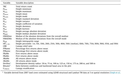
Predictor variables derived from each LiDAR point density reduction and used in multiple regression models for estimating plot-level biomass.
Variable Variable description TRC Total return count Hmin Height minimum
Hmax Height maximum
Hmean Height mean
Hmode Height mode
HSD Height standard deviation
Hvar Height variance
Hcv Height coefficient of variation
Hske Height skewness
Hkur Height kurtosis
HAAD Height average absolute deviation
HMAD Height median absolute deviation
HMADme Median of the absolute deviations from the overall median HMADMo Median of the absolute deviations from the overall mode HIQR Height interquartile range
HP(1–99) Height percentile: 1st, 5th, 10th, 20th, 25th, 30th, 40th, 50th (median), 60th, 70th, 75th, 80th, 90th, 95th, and 99th
CRR Canopy relief ratio
PFRame Percentage first returns above mean PFRamo Percentage first returns above mode FRaMe First returns above mean
FRaMo First returns above mode ARaMe All returns above mean ARaMo All returns above mode DevDena
Development density radius: 50 m, 75 m, 100 m, 125 m, 150 m, 175 m, 200 m, and 500 m BAratiob
Ratio between coniferous and hardwood basal area in the plot CSTRATA Canopy stratification
a
Variable derived from 2007 land cover estimated using LiDAR structural and Landsat TM data at 5 m spatial resolution (Singh et al., 2012).
of the relationship between biomass and canopy structural com-plexity of the urban forests.
We implemented the MLR analyses in three steps: (1) identifi-cation of outliers, (2) variable selection followed by data transfor-mation if needed, and (3) model development and performance evaluation. We started by identifying a list of LiDAR metrics (Table 3) from previous studies that are the best predictors of plot-level biomass in order to simplify the variable selection pro-cess (Dubayah et al., 2010; Frazer et al., 2011; García et al., 2010; Hall et al., 2005). We applied the variance inflation factor (VIF) and the Pearson correlation coefficients to select optimal PVs for MLR that minimized data dimensionality and the presence of mul-ticollinearity within the PVs, and to overcome issues of over fitting. Due to many potential non-collinear PVs, we also applied an
automated approach by employing the ‘regsubsets’ function from the LEAPS package (Lumley and Lumley, 2013) in the R statistical software (R Core Team, 2013) to view ranked models based on dif-ferent scoring criteria (adjusted R2, Mallows’ Cp Statistic, BIC etc.) for selecting the best regression subset (Vianna et al., 2014). We used the lowest Mallow’s Cp score, which is equivalent to the Akaike information criterion (AIC) for selecting the best subset of PVs. The AIC favors smaller residual of errors and penalizes over fit-ting a model. Therefore, lowest AIC value is ideal for selecfit-ting a model from a set of models for a given set of data. We also used logarithmic transformations during the development of the MLR models to achieve linearity between field-based biomass and non-linear forest structural parameters (Frazer et al., 2011; Hudak et al., 2006; Lefsky et al., 2002).
Fig. 3a.Predicted versus observed aboveground biomass at each LiDAR point density reduction.
2.7. Evaluating model performance
We compared the performance of MLR models using anadjusted R2, the AIC, and root mean squared error (RMSE) based on a 10-fold cross validation (k-fold CV) analysis. Theadjusted R2is the percent-age of variation explained by those PVs that influence the response variable. Theadjusted R2corrects upward bias, especially in small samples. We used the AIC to evaluate the performance of biomass models resulting from development density with increasing radii around each plot. Since biomass models comprised of relatively low number of observations (for example, 22 deciduous, 23 conif-erous, and 25 mixed plots in Forest Type models), we selected the
k-fold CV method to assess the accuracy followingNaesset (2002). In this approach, the dataset is divided intoksubsets, and at each iteration, one of theksubsets is used as testing data and the other k1 subset as training data. The variance of the resulting estimate is reduced askis increased. We also usedF-test to determine if the variance of observed biomass was equal to biomass estimated using PVs of reduced point densities.
3. Results
3.1. LiDAR point density effects on Urban Forest biomass model performance
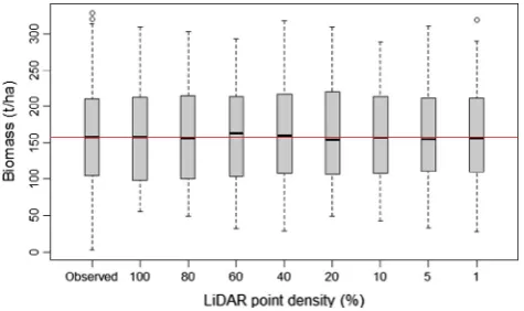
We observed similar biomass predictions for Urban Forest across all the reduced LiDAR point densities. The amount of bio-mass variance (adjusted R2) explained by LiDAR-derived PVs was consistent across the reduced point densities (Fig. 3a) with the highest difference of 11.5% observed between the 100% and 1% point density biomass models. The RMSE andk-fold CV values of Urban Forest models showed a similar trend with the maximum difference of 8.2 t/ha and 9.6 t/ha, respectively (Fig. 3b;Table 4). The biomass estimates from the 40% point density models were similar to the 100% point density except for the significance of thePFRamevariable (Table 3).PFRamewas present in all models below 80% point density, with the exception of the 1% model. The biomass variance across the reduced point densities was best explained by the tree height variance (Hvar(>60%)), followed by height percentile (HP(1–99)),percentage of first returns above mean (PFRame) (if significant in the model), and the median of the
Fig. 3b.Change inadjusted R2
and RMSE (root mean square error) across reduced LiDAR point densities.
Table 4
Multiple linear regression models for predicting aboveground biomass of urban forests using predictor variables derived from original LiDAR data and point density reductions (by percentage).
LiDARa Urban Forest model with coefficients R2 R2adjusted RMSE (t/ha) Xvalb(t/ha) F-testc
100 y= 44.39 + 0.31Hvar–3.72HMADmo+ 3.46HP05 0.8203 0.8114 31.99 34.02 (F1, 63= 1.21,p= 0.43,CI= 0.74/1.99)
80 y= 49.26 + 0.31Hvar–3.65HMADmo+ 3.28HP05 0.8086 0.7992 33.02 35.34 (F1, 63= 1.24,p= 0.39,CI= 0.75/2.03)
60 y= 5.40 + 0.28Hvar–2.58HMADmo⁄⁄ + 3.12HP05+ 0.62PFRame 0.8076 0.7948 33.10 36.93 (F1, 63= 1.24,p= 0.39,CI= 0.75/2.03)
40 y= 11.13 + 0.28Hvar–3.36HMADmo+ 2.67HP05+ 0.75PFRame⁄ 0.8210 0.8090 31.94 34.06 (F1, 63=1.22,p= 0.43,CI= 0.74/1.99)
20 y= 26.16 + 0.28Hvar–3.44HMADmo+ 2.70HP05+ 0.51PFRame 0.7872 0.7730 34.82 37.58 (F1, 63= 1.27,p= 0.34,CI= 0.77/2.08)
10 y= 19.57 + 0.27Hvar–3.64HMADmo⁄ + 2.84HP05+ 0.62PFRame 0.7747 0.7597 35.82 38.87 (F1, 63= 1.29,p= 0.30,CI =0.79/2.12)
5 y= 34.12 + 0.28Hvar–3.47HMADmo⁄ + 2.30HP05+ 0.56PFRame 0.7624 0.7466 36.79 39.35 (F1, 63= 1.31,p= 0.28,CI= 0.80/2.15)
1 y=119.15 + 1.27TRC⁄ + 2.56Hmin+ 0.17Hvar+ 259.90CRR 0.7164 0.6975 40.19 43.63 (F1, 63= 1.40,p= 0.18,CI= 0.85/2.29)
Level of significance: 0.001 ‘⁄⁄
’ 0.01 ‘⁄
’ 0.05 ‘’ 0.1.
a
Percentage of original LiDAR data.
b
10-fold cross validation.
c
Between observed and predicted aboveground biomass.
absolute deviations from the overall mode (HMADMo). F-tests (equality of two variances) revealed no significant differences between the observed and predicted biomass estimates (Table 4) with virtually consistent distributions across the models except for slight differences at the 60% and 20% LiDAR point densities (Fig. 4).
3.2. Performance of Forest Type biomass model
While Urban Forest biomass models performed consistently well across the reduced point densities, due to similar adjusted
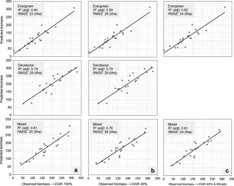
R2, we selected 100% and 40% point densities for developing Forest Type biomass models. Forest Type biomass models outperformed (individually as well as cumulatively) the Urban Forest models at both the 100% and 40% point densities. Forest Type biomass mod-els produced, on average, 4–6 t/ha lower RMSE values than Urban Forest models. The evergreen biomass model based on the 100% point density produced the highestadjusted R2and lowest RMSE followed by mixed and deciduous types (Fig. 5;Table 5). We found a moderate but significant difference in evergreen and mixed types biomass variance (on average 4.56%) between the 100% and 40% point densities (Fig. 5) except for the deciduous type which
Fig. 5.Predicted versus observed aboveground biomass by Forest Type: (a) model based on 100% point density, (b) model based on 40% point density, and (c) effect of basal area ratio (BAratio) on the evergreen and mixed Forest Type biomass models of 40% point density.
Table 5
Multiple linear regression models for predicting aboveground biomass of different Forest Types using 100% and 40% point densities.
LiDARa Forest type Coefficients R2 R2adjusted RMSE (t/ha)
100 Evergreen y=65.62 + 0.03TRC+ 27.08Hmin+ 0.32Hvar–4.58HMADmo 0.8681 0.8371 23.37
Deciduous y= 178.85 + 0.30Hvar–73.78In(HMADmo)+ 3.38HP05 0.8267 0.7942 29.13
Mixed y= 121.89–79.20In(TRC)+ 0.15Hvar–15.30HP01+ 4.76HP05 0.8490 0.8135 24.79
40 Evergreen y=239.07 + 40In(TRC)+ 0.25Hvar–2.67HMADmo+ 8.21HP01 0.8362 0.7977 26.05
Deciduous y= 210.21 + 0.31Hvar–83.92In(HMADmo)+ 2.98HP05 0.8257 0.7930 29.22
Mixed y= 73.12–0.04TRC+ 0.25Hvar–8.48HP01+ 6.54HP05 0.8056 0.7598 28.13
40b
Evergreen y=370.27 + 52.7In(TRC)+ 0.25Hvar–2.69HMADmo+ 29.53Hmin–0.79BAratio 0.8599 0.8161 24.09
Mixed y =129.12–0.05TRC+ 0.23Hvar–8.90HP01+ 5.94HP05–89.23BAratio⁄ 0.8555 0.8104 24.25
Level of significance: 0.01 ‘⁄
’ 0.05 ‘’ 0.1.
a Percentage of original LiDAR data.
b Model with basal area ratio (BAratio) variable.
showed similaradjusted R2(79%) and RMSE (29 t/ha) values. Bio-mass estimates of evergreen and mixed models performed simi-larly as we introduced the basal area ratio variable into the models. The average difference of RMSE values of Forest Type bio-mass models based on 100% and 40% point densities was 2 t/ha. However, we observed a difference of 6.2 t/ha and 5 t/ha at 100% and 40% densities, respectively, between Urban Forest and the combined estimates of Forest Type models (Table 5).
3.3. Development density effects on biomass model performance
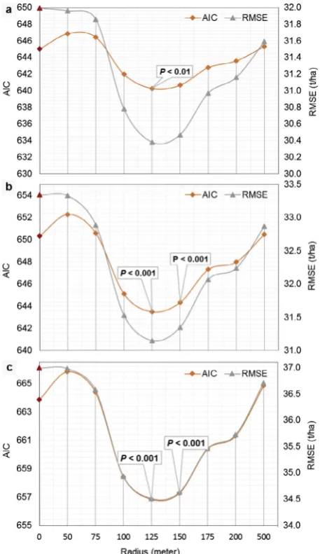
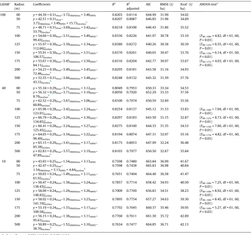
Development density exhibited a negative relationship with biomass and contributed on average 2.3% to the total explained biomass variance of models using 100%, 40%, and 10% point densi-ties. Equivalent contributions of development density suggest that development density is independent of point density and not due to chance. We achieved lower AIC and RMSE values with higher significance levels using development densities between 100 m and 175 m radius buffers, peaking at 125 m withp< 0.01 signifi-cance level for all three reduced point densities (Fig. 6a–c).Table 6
illustrates how biomass variance improved with the addition of development density. The biomass models at 125 m radius
pro-duced the highestadjusted R2(0.83, 0.82, and 0.78 at 100%, 40%, and 10% point densities, respectively) and the lowestk-fold CV-RMSE values (30.4 t/ha, 32.9 t/ha, and 38.2 t/ha at 100%, 40%, and 10%, respectively). Analysis of variance (ANOVA) tests revealed that biomass models using development densities at 100 m, 125 m, 150 m, and 175 m are significantly different from the mod-els that exclude development density at all three reduced point densities (Table 6).
3.4. Contribution of canopy stratification on biomass estimation
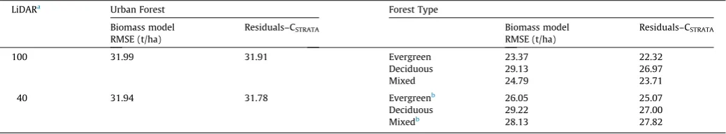
Canopy stratification did not contribute to the Urban Forest bio-mass model and only marginally improved the unexplained vari-ance of the Forest Type biomass models. On average, the canopy stratification improved Forest Type biomass models by 1.4 t/ha and 1.2 t/ha at 100% and 40% point densities, respectively; the deciduous model showed the greatest improvement of 2.2 t/ha at both densities (Table 7).
4. Discussion
Accurate and repeated biomass estimation over large urbaniz-ing areas has become a necessity to manage remnant forests and their potential impacts on regional carbon dynamics. This research explored the effects of LiDAR point density and landscape context on the accuracy of biomass estimates in urban remnant forests at a regional-scale. We found that reducing point density provided a viable solution to regional-scale assessment without compromis-ing accuracy of biomass estimates. Differences inadjusted R2and RMSE values between 100% and 1% LiDAR point density cases were modest and disproportionate to the reduction in average point spacing and file size (Table 1).Jakubowski et al. (2013)found sim-ilar results and suggested that the accuracy of predicted forest structure metrics remains relatively high until low point densities are incorporated in the model. In addition, we were unable to extract many important LiDAR metrics below 1% data reduction, and therefore we used 1% as the cut-off for the analysis. These raise two important methodological questions not addressed in this cur-rent study. First, what is the minimum number of points required to represent the three-dimensional structure sufficiently to pro-vide suitable metrics for accurate biomass estimation? Second, how to reduce LiDAR data without compromising the quality of structural attributes? In this study, the data reduction algorithm and the structural predictors contributed to the performance of biomass estimation across the reduced point densities.
LiDAR data reduction by the ‘percentage of the total points’ algorithm was selected over the ‘point density’ and ‘point spacing’ algorithms since the latter two methods vary tile to tile and are determined by the complexities found in forest stands. For exam-ple, the overall point spacing for the county-level LiDAR data was 1 m, while plot-level LiDAR data reduced to 20% density produced the equivalent point spacing.Table 1 shows that LiDAR data at lower point densities decreased the average point spacing dispro-portionately in comparison to reductions in file size. These findings are consistent withAnderson et al. (2006)in that the reduction of LiDAR data to a certain extent does not affect the statistical prop-erties of the elevation models. Therefore, LiDAR data can be reduced without significantly impacting the accuracy of biomass estimates. For example, models using 40% LiDAR point density with a significant reduction in density, spacing, and file size pro-duced comparable biomass estimates to models using the full LiDAR dataset (Table 1). Our study is based on the Charlotte Metro-politan Area where the best data point density may not be the best for other geographic regions of varying urban development densi-ties and spatial patterns. This baseline research offers a feasibility
of reducing data acquisition costs and volume while retaining the accuracy of forest biomass estimates in complex urban environ-ments. Largely, such data reduction can considerably minimize data processing time for large-area assessments without compro-mising the accuracy of biomass estimates. Point density reductions may lower data costs for large-area assessments, especially in cases where repeated coverage is needed.
The cumulative Forest Type biomass model outperformed the Urban Forest model at both 100% and 40% point densities. The observed variability in model performance across the three forest types at both point densities corroborate the findings of Zolkos
et al. (2013). The structural complexities (e.g., canopy stratifica-tion, presence of understory vegetastratifica-tion, canopy density, etc.) of forest strata are one potential source of variability in model perfor-mance. Other issues, such as leaf-on vs. leaf-off LiDAR data, also impact model performance.Naesset (2005)reported that the vari-ability of the height distribution tends to increase from leaf-on to leaf-off conditions, which may cause variation in biomass esti-mates. This research utilized leaf-off data, and so this effect could not be evaluated. Likewise, less variation in the heights of conifers could lead to higher accuracies for biomass estimates in coniferous stands compared with hardwood stands (Nelson et al., 2004). This
Table 6
Contribution of development density, derived at nine different radii, in the regression models for predicting aboveground biomass using predictor variables derived at 100%, 40%, and 10% LiDAR point densities.
LiDARa
Radius (m)
Coefficients R2
R2
adjusted
AIC RMSE (t/ ha)
Xvalc
(t/ ha)
ANOVA-testd
100 00 y= 44.39 + 0.31Hvar–3.72HMADmo+ 3.46HP05 0.8203 0.8114 644.99 31.99 34.02
50 y= 42.51 + 0.31Hvar–
3.72HMADmo+ 3.49HP05+ 15.73DevDenb
0.8207 0.8087 646.85 31.96 34.69 75 y= 48.71 + 0.31Hvar–3.69HMADmo+ 3.42HP05–
33.79DevDenb
0.8218 0.8100 646.43 31.86 35.52 100 y= 54.60 + 0.30Hvar–3.51HMADmo+ 3.49HP05–
99.43DevDen⁄
0.8336 0.8226 641.97 30.78 33.10 (F00–100r= 4.82, df = 61, 60,
P= 0.03) 125 y= 55.97 + 0.30Hvar–3.39HMADmo+ 3.34HP05–
112.66DevDen⁄⁄
0.8380 0.8272 640.26 30.38 30.39 (F00–125r= 6.55, df = 61, 60,
P= 0.01) 150 y= 55.91 + 0.30Hvar–3.35HMADmo+ 3.51HP05–
106.57DevDen⁄
0.8370 0.8261 640.65 30.47 33.76 (F00–150r= 6.14, df = 61, 60,
P= 0.01) 175 y= 53.67 + 0.30Hvar–3.45HMADmo+ 3.50HP05–
84.11DevDen⁄
0.8316 0.8204 642.77 30.97 33.67 (F00–175r= 4.03, df = 61, 60,
P= 0.05) 200 y= 54.23 + 0.30Hvar–3.49HMADmo+ 3.45HP05–
72.48DevDenb
0.8295 0.8181 643.58 31.16 34.93 500 y= 52.55 + 0.31Hvar–3.66HMADmo+ 3.48HP05–
43.33DevDenb
0.8248 0.8132 645.32 31.59 37.76
40 00 y= 55.34 + 0.29Hvar–3.71HMADmo+ 3.12HP05 0.8049 0.7953 650.33 33.34 34.53
50 y= 56.32 + 0.29Hvar–3.71HMADmo+ 3.10HP05–
8.70DevDenb
0.8050 0.7920 652.29 33.33 37.56 75 y= 62.52 + 0.29Hvar–3.67HMADmo+ 3.06HP05–
60.89DevDenb
0.8100 0.7974 650.59 32.89 35.56 100 y= 65.96 + 0.28Hvar–3.42HMADmo+ 3.24HP05–
123.91DevDen⁄
0.8254 0.8137 645.12 31.53 33.83 (F00–100r= 7.04, df = 61, 60,
P= 0.01) 125 y= 66.79 + 0.28Hvar–3.29HMADmo+ 3.30HP05–
134.85DevDen⁄⁄
0.8297 0.8183 643.50 31.15 32.87 (F00–125r= 8.73, df = 61, 60,
P= 0.01) 150 y= 66.41 + 0.28Hvar–3.24HMADmo+ 3.27HP05–
125.45DevDen⁄⁄
0.8275 0.8160 644.33 31.35 34.53 (F00–150r= 7.86, df = 61, 60,
P= 0.01) 175 y= 64.03 + 0.29Hvar–3.34HMADmo+ 3.22HP05–
96.49DevDen⁄
0.8194 0.8074 647.31 32.07 35.16 (F00–175r= 4.82, df = 61, 60,
P= 0.03) 200 y= 65.15 + 0.29Hvar–3.41HMADmo+ 3.17HP05–
85.38DevDen ⁄
0.8175 0.8053 647.99 32.24 36.48 500 y= 62.83 + 0.29Hvar–3.57HMADmo+ 3.19HP05–
47.89DevDenb
0.8103 0.7977 650.50 32.87 35.84
10 00 y= 43.03 + 0.25Hvar–1.54HMADmo+ 3.13HP05 0.7598 0.7480 663.84 36.99 41.67
50 y= 42.47 + 0.25Hvar–
1.54HMADmo+ 3.13HP05+ 4.84DevDenb
0.7598 0.7438 665.83 36.98 40.84 75 y= 50.03 + 0.24Hvar–1.49HMADmo+ 3.11HP05–
61.92DevDenb
0.7651 0.7494 664.40 36.58 41.47 100 y= 56.47 + 0.24Hvar–1.38HMADmo+ 3.24HP05–
138.43DevDen⁄⁄
0.7857 0.7714 658.42 34.93 40.50 (F00–100r= 7.25, df = 61, 60,
P= 0.01) 125 y= 58.09 + 0.24Hvar–1.29HMADmo+ 3.26HP05–
148.82DevDen⁄⁄
0.7909 0.7769 656.83 34.51 38.23 (F00–100r= 8.92, df = 61, 60,
P= 0.01) 150 y= 58.02 + 0.24Hvar–1.26HMADmo+ 3.23HP05–
141.19DevDen⁄⁄
0.7895 0.7754 657.27 34.63 39.30 (F00–100r= 8.45, df = 61, 60,
P= 0.01) 175 y= 55.19 + 0.24Hvar–1.33HMADmo+ 3.17HP05–
109.58DevDen⁄
0.7792 0.7645 660.37 35.46 39.95 (F00–100r= 5.27, df = 61, 60,
P= 0.03) 200 y= 56.15 + 0.24Hvar–1.38HMADmo+ 3.11HP05–
95.61DevDen⁄
0.7760 0.7611 661.30 35.72 42.89 500 y= 50.89 + 0.25Hvar–1.52HMADmo+ 3.10HP05–
38.70DevDenb
0.7634 0.7477 664.85 36.71 42.13
Level of significance: 0.001 ‘⁄⁄
’ 0.01 ‘⁄
’ 0.05 ‘’ 0.1.
a
Percentage of original LiDAR data.
b
Insignificant in the model.
c
10-fold cross validation.
d
Between models with and without development density.
disparity may also depend upon the height to biomass relationship difference between hardwood (more biomass in branches) and conifer species (Nelson et al., 2007). However, differences in the performance of the Forest Type (evergreen and mixed) models using 100% and 40% of LiDAR data were unexpected. Adding the ‘basal area ratio’ variable to these models resulted in similar esti-mates, suggesting that the reduced point density does not fully explain the complexity found in the lower strata of evergreen trees in urban remnant forests either in evergreen or mixed forest type field plots. This is a significant finding given the prevalence of coni-fers in the study system, making ‘basal area ratio’ an important variable to compensate effectively for low point densities in the evergreen and mixed forest type biomass models.
Urbanization alters tree growth and understory recruitment along urban–rural gradients (O’Brien et al., 2012). Evaluation of biomass models using development density at increasing radii revealed development density as an important contributor to bio-mass estimates and the quantification biobio-mass of urban remnant forests. Our results illustrate improved performance from 100 m to 175 m buffer distance, with no change beyond 175 m (Fig. 6;
Table 6). Insignificant contributions of development density to bio-mass estimation from the edge of the field plot to 100 m may be due to the deliberate distribution of field plots within forest sites with the least amount of developed land cover. The absence of a development density effect beyond175 m could be ascribed to the maximum developed land cover around each plot given the prevalence of developed land cover in this urbanizing region. To verify this significant outcome was not by chance and was inde-pendent of point density. We modeled biomass at three different LiDAR point densities (100%, 40%, and 10%) and found the same outcomes. O’Brien et al. (2012) suggested that anthropogenic impacts on urban forests could be multi-faceted, therefore, addi-tional research is required to fully understand which land cover type has more impact on forest biomass estimates along urban– rural gradients.
Evaluation of multiple linear regression models in our analysis illustrated that descriptive statistics metrics (e.g., tree-height-var-iance (Hvar)) explained more variance than direct canopy height related metrics and were overall key predictors of biomass. The second largest contributor to overall model performance was HMADMo (median of the absolute deviations from the overall mode), which is a robust measure of variability within the data sample. This implies that field-measured biomass is primarily related to overall vertical forest structure. Zimble et al. (2003)
identified tree-height-variance as an effective metric for classifying various vertical forest structural configurations. Additionally, leaf-off LiDAR has been recommended to improve the estimation accu-racy of biophysical properties and prediction in a mixed forest, with further improvements by adding forest stratification (Naesset, 2005). However, the contributions of these two variables
in overall model performance could be a potential explanation for the relatively poor performance of canopy stratification in our Urban Forest biomass model.
5. Conclusions
Management of urban remnant forests and critical ecological and environmental processes necessary to maintain ecosystem functioning and services can be enhanced by the resourceful use of LiDAR remote sensing for improved assessment of regional-scale urban forest biomass. This study advances the application of LiDAR data for effective assessment of large-area biomass. Our results suggest that reducing LiDAR point density may offer an effective solution for minimizing regional-scale data procurement costs and overcoming computational challenges while maintaining desired accuracy of biomass estimations. Our evaluation of Urban Forest models performance suggests that LiDAR data with an aver-age point spacing of 0.70–1.50 m (approximately 1.35 points/m2) may offer a cost-effective, large-area LiDAR data procurement and processing for urban forest landscapes. Equivalent biomass estimates across multiple point densities suggests the ‘percentage of the total points’ data reduction algorithm is suitable for large-area applications. Lower individual and cumulative RMSE values of the Forest Type biomass models emphasize the consideration of forest types for reasonable biomass estimates at regional-scales. As expected, land cover type impacts the productivity and growth of forests in urbanizing landscapes, and when we added develop-ment density to the biomass models, our estimates improved. We also observed that canopy stratification did not improve our biomass estimation for urban forests but did lead to a slight improvement when applied to the deciduous biomass model. This suggests complexity in the vertical strata of deciduous forests affects biomass estimation. Our evaluation of all biomass models revealed tree-height-variance as the most useful biomass predic-tor, corroborating its suitability for classifying various vertical for-est structure configurations. Overall, our findings suggfor-est that reduced density LiDAR data may lower data procurement costs for repeated assessments without sacrificing accuracy, and bio-mass estimates can be improved by including landscape character-istics (e.g., land cover types, development density, etc.) in regional analyses.
Acknowledgements
This research was supported by the Garden Club of America (GCA) Zone VI fellowship in urban forestry, the Casey Trees Endowment Fund, and the Association of American Geographers Dissertation Research grant. We are very grateful to the North Carolina Space Grant Consortium for additional financial support. We express sincere thanks to the Storm Water Services Division
Table 7
Contribution of canopy stratification in estimation of aboveground biomass for Urban Forest and Forest Type using predictor variables derived at 100% and 40% LiDAR point densities.
LiDARa
Urban Forest Forest Type
Biomass model Residuals–CSTRATA Biomass model Residuals–CSTRATA
RMSE (t/ha) RMSE (t/ha)
100 31.99 31.91 Evergreen 23.37 22.32
Deciduous 29.13 26.97
Mixed 24.79 23.71
40 31.94 31.78 Evergreenb
26.05 25.07 Deciduous 29.22 27.00 Mixedb 28.13 27.82 a
Percentage of original LiDAR data.
b
of Charlotte–Mecklenburg County government office, and Engi-neering and Property Management, Land Development Services, the City of Charlotte for providing LiDAR data. We thank students, research staff, and doctoral dissertation committee members from the Center for Geospatial Analytics, North Carolina State University, for their comments and feedback on the manuscript.
References
Anderson, E.S., Thompson, J.A., Crouse, D.A., Austin, R.E., 2006. Horizontal resolution and data density effects on remotely sensed LIDAR-based DEM. Geoderma 132 (3–4), 406–415.
Baker, P.J., Wilson, J.S., 2000. A quantitative technique for the identification of canopy stratification in tropical and temperate forests. For. Ecol. Manage. 127 (1–3), 77–86.
BCAL LiDAR Tools, Version 1.5.2, 2013. Idaho State University, Department of Geosciences, Boise Center Aerospace Laboratory (BCAL), Boise, Idaho. <http:// bcal.geology.isu.edu/envitools.shtml>.
Chen, G., Hay, G.J., 2011. An airborne lidar sampling strategy to model forest canopy height from Quickbird imagery and GEOBIA. Remote Sens. Environ. 115 (6), 1532–1542.
Dixon, G., 2002. Essential FVS: A User’s Guide to the Forest Vegetation Simulator. U.S. Department of Agriculture, Forest Service, Forest Managment Service Center, Fort Collins, CO.
Drake, J.B., Dubayah, R.O., Knox, R.G., Clark, D.B., Blair, J.B., 2002. Sensitivity of large-footprint lidar to canopy structure and biomass in a neotropical rainforest. Remote Sens. Environ. 81 (2–3), 378–392.
Drake, J.B., Knox, R.G., Dubayah, R.O., Clark, D.B., Condit, R., Blair, J.B., Hofton, M., 2003. Above-ground biomass estimation in closed canopy neotropical forests using lidar remote sensing: factors affecting the generality of relationships. Glob. Ecol. Biogeogr. 12 (2), 147–159.
Dubayah, R.O., Sheldon, S.L., Clark, D.B., Hofton, M.A., Blair, J.B., Hurtt, G.C., Chazdon, R.L., 2010. Estimation of tropical forest height and biomass dynamics using lidar remote sensing at La Selva, Costa Rica. J. Geophys. Res. 115, G00E09.
Estornell, J., Ruiz, L.A., Velazquez-Marti, B., Fernandez-Sarria, A., 2011. Estimation of shrub biomass by airborne LiDAR data in small forest stands. For. Ecol. Manage. 262 (9), 1697–1703.
Frazer, G.W., Magnussen, S., Wulder, M.A., Niemann, K.O., 2011. Simulated impact of sample plot size and co-registration error on the accuracy and uncertainty of LiDAR-derived estimates of forest stand biomass. Remote Sens. Environ. 115 (2), 636–649.
Garcia, M., Riano, D., Chuvieco, E., Danson, F.M., 2010. Estimating biomass carbon stocks for a Mediterranean forest in central Spain using LiDAR height and intensity data. Remote Sens. Environ. 114 (4), 816–830.
García, M., Riaño, D., Chuvieco, E., Danson, F.M., 2010. Estimating biomass carbon stocks for a Mediterranean forest in central Spain using LiDAR height and intensity data. Remote Sens. Environ. 114 (4), 816–830.
Gobakken, T., Naesset, E., 2008. Assessing effects of laser point density, ground sampling intensity, and field sample plot size on biophysical stand properties derived from airborne laser scanner data. Can. J. For. Res. 38 (5), 1095–1109.
Godwin, C., Chen, G., Singh, K.K., 2015. The impact of urban residential development patterns on forest carbon density: An integration of LiDAR aerial photography and field mensuration. Landscape Urban Plan. 136, 97–109.
Gregg, J.W., Jones, C.G., Dawson, T.E., 2003. Urbanization effects on tree growth in the vicinity of New York City. Nature 424 (6945), 183–187.
Groffman, P.M., Pouyat, R.V., Cadenasso, M.L., Zipperer, W.C., Szlavecz, K., Yesilonis, I.D., Band, L.E., Brush, G.S., 2006. Land use context and natural soil controls on plant community composition and soil nitrogen and carbon dynamics in urban and rural forests. For. Ecol. Manage. 236 (2–3), 177–192.
Grove, J.M., Troy, A.R., O’Neil-Dunne, J.P.M., Burch, W.R., Cadenasso, M.L., Pickett, S.T.A., 2006. Characterization of households and its implications for the vegetation of urban ecosystems. Ecosystems 9 (4), 578–597.
Hall, S.A., Burke, I.C., Box, D.O., Kaufmann, M.R., Stoker, J.M., 2005. Estimating stand structure using discrete-return lidar: an example from low density, fire prone ponderosa pine forests. For. Ecol. Manage. 208 (1–3), 189–209.
He, C., Convertino, M., Feng, Z.K., Zhang, S.Y., 2013. Using LiDAR data to measure the 3D green biomass of Beijing urban forest in China. PLoS ONE 8 (10).
Hudak, A.T., Crookston, N.L., Evans, J.S., Falkowski, M.J., Smith, A.M.S., Gessler, P.E., Morgan, P., 2006. Regression modeling and mapping of coniferous forest basal area and tree density from discrete-return lidar and multispectral satellite data. Can. J. Remote Sens. 32 (2), 126–138.
Imhoff, M.L., Zhang, P., Wolfe, R.E., Bounoua, L., 2010. Remote sensing of the urban heat island effect across biomes in the continental USA. Remote Sens. Environ. 114 (3), 504–513.
Jakubowski, M.K., Guo, Q.H., Kelly, M., 2013. Tradeoffs between lidar pulse density and forest measurement accuracy. Remote Sens. Environ. 130, 245–253.
Jenkins, J.C., Chojnacky, D.C., Heath, L.S., Birdsey, R.A., 2003. National-scale biomass estimators for United States tree species. Forest Sci. 49 (1), 12–35.
Lefsky, M.A., Cohen, W.B., Harding, D.J., Parker, G.G., Acker, S.A., Gower, S.T., 2002. Lidar remote sensing of above-ground biomass in three biomes. Glob. Ecol. Biogeogr. 11 (5), 393–399.
Lim, K., Hopkinson, C., Treitz, P., 2008. Examining the effects of sampling point densities on laser canopy height and density metrics. Forestry Chronicle 84 (6), 876–885.
Lovell, J.L., Jupp, D.L.B., Newnham, G.J., Coops, N.C., Culvenor, D.S., 2005. Simulation study for finding optimal lidar acquisition parameters for forest height retrieval. For. Ecol. Manage. 214 (1–3), 398–412.
Lumley, T., Lumley, M.T., 2013. Package ‘leaps’.
Magnani, F., Mencuccini, M., Borghetti, M., Berbigier, P., Berninger, F., Delzon, S., Grelle, A., Hari, P., Jarvis, P.G., Kolari, P., Kowalski, A.S., Lankreijer, H., Law, B.E., Lindroth, A., Loustau, D., Manca, G., Moncrieff, J.B., Rayment, M., Tedeschi, V., Valentini, R., Grace, J., 2007. The human footprint in the carbon cycle of temperate and boreal forests. Nature 447 (7146), 848–850.
Magnusson, M., Fransson, J.E.S., Holmgren, J., 2007. Effects on estimation accuracy of forest variables using different pulse density of laser data. Forest Sci. 53 (6), 619–626.
Mascaro, J., Detto, M., Asner, G.P., Muller-Landau, H.C., 2011. Evaluating uncertainty in mapping forest carbon with airborne LiDAR. Remote Sens. Environ. 115 (12), 3770–3774.
McCarter, J.B., 2001. Landscape Management System (lms): Background, Methods, and Computer Tools for Integrating Forest Inventory, gis, Growth and Yield, Visualization and Analysis for Sustaining multiple forest objectives. University of Washington, pp. 101.
McCarter, J.B., Wilson, J.S., Baker, P.J., Moffett, J.L., Oliver, C.D., 1998. Landscape management through integration of existing tools and emerging technologies. J. Forest. 96 (6), 17–23.
McGaughey, R.J., Version 3.42, 2014. FUSION/LDV: Software for LIDAR Data Analysis and Visualization. U.S. Department of Agriculture, Forest Service, Pacific Northwest Research Station, Seattle, WA, <http://forsys.cfr.washington.edu/ fusion/fusionlatest.html>.
McHale, M., Burke, I., Lefsky, M., Peper, P., McPherson, E., 2009. Urban forest biomass estimates: is it important to use allometric relationships developed specifically for urban trees? Urban Ecosyst. 12 (1), 95–113.
Meentemeyer, R.K., Tang, W.W., Dorning, M.A., Vogler, J.B., Cunniffe, N.J., Shoemaker, D.A., 2013. FUTURES: multilevel simulations of emerging urban-rural landscape structure using a stochastic patch-growing algorithm. Ann. Assoc. Am. Geogr. 103 (4), 785–807.
Moran, M.A., 1984. Influence of adjacent land use on understory vegetation of New York forests. Urban Ecol. 8 (4), 329–340.
Naesset, E., 2002. Predicting forest stand characteristics with airborne scanning laser using a practical two-stage procedure and field data. Remote Sens. Environ. 80 (1), 88–99.
Naesset, E., 2005. Assessing sensor effects and effects of leaf-off and leaf-on canopy conditions on biophysical stand properties derived from small-footprint airborne laser data. Remote Sens. Environ. 98 (2–3), 356–370.
Naesset, E., 2009. Effects of different sensors, flying altitudes, and pulse repetition frequencies on forest canopy metrics and biophysical stand properties derived from small-footprint airborne laser data. Remote Sens. Environ. 113 (1), 148–159.
Nelson, R., Short, A., Valenti, M., 2004. Measuring biomass and carbon in Delaware using an airborne profiling LIDAR. Scand. J. For. Res. 19 (6), 500–511.
Nelson, R.F., Hyde, P., Johnson, P., Emessiene, B., Imhoff, M.L., Campbell, R., Edwards, W., 2007. Investigating RaDAR-LiDAR synergy in a North Carolina pine forest. Remote Sens. Environ. 110 (1), 98–108.
Nowak, D.J., Greenfield, E.J., 2012. Tree and impervious cover change in US cities. Urban Forestry & Urban Greening 11 (1), 21–30.
O’Brien, A.M., Ettinger, A.K., HilleRisLambers, J., 2012. Conifer growth and reproduction in urban forest fragments: predictors of future responses to global change? Urban Ecosyst. 15 (4), 879–891.
Parker, G.G., Brown, M.J., 2000. Forest canopy stratification – is it useful? Am. Nat. 155 (4), 473–484.
Popescu, S.C., 2007. Estimating biomass of individual pine trees using airborne lidar. Biomass Bioenergy 31 (9), 646–655.
Popescu, S.C., Wynne, R.H., Scrivani, J.A., 2004. Fusion of small-footprint lidar and multispectral data to estimate plot-level volume and biomass in deciduous and pine forests in Virginia, USA. Forest Sci. 50 (4), 551–565.
R Core Team, 2013. R: A Language and Environment for Statistical Computing, R Foundation for Statistical Computing, Vienna, Austria. <http://www.R-project. org/>.
Renslow, M., Greenfield, P., Guay, T., 2000. Evaluation of Multi-return LIDAR for Forestry Applications. RSAC-2060/4810-LSP-0001-RPT1. US Department of Agriculture Forest Service — Remote Sensing Applications Center, pp. 12.
Seidel, D., Albert, K., Fehrmann, L., Ammer, C., 2012. The potential of terrestrial laser scanning for the estimation of understory biomass in coppice-with-standard systems. Biomass Bioenergy 47, 20–25.
Seto, K.C., Guneralp, B., Hutyra, L.R., 2012. Global forecasts of urban expansion to 2030 and direct impacts on biodiversity and carbon pools. Proc. Natl. Acad. Sci. U.S.A. 109 (40), 16083–16088.
Singh, K.K., Vogler, J.B., Shoemaker, D.A., Meentemeyer, R.K., 2012. LiDAR-Landsat data fusion for large-area assessment of urban land cover: balancing spatial resolution, data volume and mapping accuracy. ISPRS J. Photogrammet. Remote Sens. 74, 110–121.
Stage, A., 1973. Prognosis Model for Stand Development. Research Paper INT-137. U.S. Department of Agriculture, Forest Service, Intermountain Forest and Range Experiment Station, Ogden, UT.
Swatantran, A., Dubayah, R., Roberts, D., Hofton, M., Blair, J.B., 2011. Mapping biomass and stress in the Sierra Nevada using lidar and hyperspectral data fusion. Remote Sens. Environ. 115 (11), 2917–2930.
Treitz, P., Lim, K., Woods, M., Pitt, D., Nesbitt, D., Etheridge, D., 2012. LiDAR sampling density for forest resource inventories in Ontario, Canada. Remote Sens. 4 (4), 830–848.
Vianna, G.M.S., Meekan, M.G., Bornovski, T.H., Meeuwig, J.J., 2014. Acoustic telemetry validates a citizen science approach for monitoring sharks on coral reefs. PLoS ONE 9 (4).
Wykoff, W.R., Crookston, N.L., Stage, A.R., 1982. User’s Guide to the Stand Prognosis Model. General Technical Report INT-122. U.S. Department of Agriculture, Forest Service, Intermountain Forest and Range Experiment Station, Ogden, UT.
Zhao, K., Popescu, S., Nelson, R., 2009. Lidar remote sensing of forest biomass: a scale-invariant estimation approach using airborne lasers. Remote Sens. Environ. 113 (1), 182–196.
Zimble, D.A., Evans, D.L., Carlson, G.C., Parker, R.C., Grado, S.C., Gerard, P.D., 2003. Characterizing vertical forest structure using small-footprint airborne LiDAR. Remote Sens. Environ. 87 (2–3), 171–182.