ABSTRACT
JIN, LU. Essays on Window Selection for Out-of-sample Forecasting. (Under the direction of Atsushi Inoue.)
Forecasting is a common practice in academia, government and business alike, and accuracy of forecasts is crucial for policy makers and decision makers. However, practitioners are often left wondering how to choose the sample for estimating forecasting models. For example, when we forecast inflation in 2014, should we use the last 30 years of data or the last 10 years of data? In the presence of possible structural changes in economic time series, forecasting performance is often quite sensitive to the choice of such “window size”. The aim of this dissertation is to provide practical solutions for determining how many most recent observations to include in estimation for forecasting mean and quantiles of a variable.
In the first chapter, we develop a novel method for selecting the estimation window size for forecasting means. Specifically, we propose to choose the window size that minimizes the forecaster’s quadratic loss function, and we prove the asymptotic validity of our approach. The forecasting models are assumed to be linear in smoothly time-varying parameters. Our approach uses local linear regressions to approximate the infeasible loss function. The Monte Carlo experiments show that the proposed method performs quite well under various types of structural changes. When applied to forecast US real output growth and inflation, the proposed method tends to improve upon conventional methods.
© Copyright 2014 by Lu Jin
Essays on Window Selection for Out-of-sample Forecasting
by Lu Jin
A dissertation submitted to the Graduate Faculty of North Carolina State University
in partial fulfillment of the requirements for the Degree of
Doctor of Philosophy
Economics
Raleigh, North Carolina
2014
APPROVED BY:
Barry K. Goodwin Denis Pelletier
Wenbin Lu Atsushi Inoue
DEDICATION
BIOGRAPHY
ACKNOWLEDGEMENTS
TABLE OF CONTENTS
LIST OF TABLES . . . vii
LIST OF FIGURES . . . .viii
Chapter 1 Window Selection for Out-of-Sample Forecasting with Time-Varying Parameters . . . 1
1.1 Introduction . . . 1
1.2 Theory . . . 4
1.2.1 Assumptions . . . 5
1.2.2 Infeasible Conditional MSFE . . . 7
1.2.3 Approximate MSFE using Local Linear Regressions . . . 8
1.3 Monte Carlo Experiments . . . 10
1.3.1 DGPs . . . 10
1.3.2 Window Selection Methods . . . 11
1.3.3 Simulation Results . . . 12
1.4 Empirical Analysis . . . 16
1.4.1 Data . . . 16
1.4.2 Forecasting Models . . . 17
1.4.3 Results . . . 17
1.5 Discussion and Conclusion . . . 19
Chapter 2 Automatic Window Selection in Quantile Forecasting . . . 36
2.1 Introduction . . . 36
2.2 Model Specifications and Estimation . . . 39
2.2.1 Notations . . . 39
2.2.2 Setup . . . 39
2.2.3 Nonlinear Quantile Regression . . . 45
2.3 Window Selection Approach . . . 45
2.4 Monte Carlo Simulations . . . 47
2.4.1 DGPs . . . 47
2.4.2 Simulation Results . . . 49
2.5 Empirical Application: Forecasting Intervals of Future Commodity Prices . . . . 50
2.5.1 Background . . . 50
2.5.2 Data Characteristics . . . 52
2.5.3 Forecasting Models . . . 53
2.5.4 Results . . . 56
2.6 Conclusion . . . 59
References. . . 84
Appendices . . . 89
Appendix A Appendix of Chapter 1 . . . 90
A.2 Definitions . . . 90
A.3 Proofs of Theorems . . . 91
A.4 Proofs of Lemmas . . . 93
A.5 Results for Empirical Analysis . . . 116
Appendix B Appendix of Chapter 2 . . . 135
B.1 Proofs of Theorems . . . 135
B.2 Proof of Lemmas . . . 142
LIST OF TABLES
Table 1.1 Definition of ΘR . . . 10
Table 1.2 Description of DGPs . . . 21
Table 1.3 Root MSFE (T=100) . . . 22
Table 1.4 Root MSFE (T=200) . . . 23
Table 1.5 Average Window Size Across Monte Carlo Replications (T=100) . . . 24
Table 1.6 Average Window Size Across Monte Carlo Replications (T=200) . . . 25
Table 1.7 Data Description . . . 26
Table 1.8 Pseudo Rolling Out-of-Sample Forecasts of the Real GDP Growth Rate . . . 28
Table 1.9 Pseudo Rolling Out-of-Sample Forecasts of Inflation . . . 30
Table 2.1 Description of DGPs . . . 60
Table 2.2 Relative Mean Quantile Error of Model A: T=100 . . . 61
Table 2.3 Relative Mean Quantile Error of Model A: T=200 . . . 62
Table 2.4 Average of Optimal Window Size for Model A: T=100, 200 . . . 63
Table 2.5 Relative Mean Quantile Error of Model B: T=100 . . . 64
Table 2.6 Relative Mean Quantile Error of Model B: T=200 . . . 65
Table 2.7 Average of Optimal Window Size for Model B: T=100, 200 . . . 66
Table 2.8 Data Description . . . 67
Table 2.9 Commodity Spot Price Features 1960Q1-2011Q4 . . . 68
Table 2.10 Mean Quantile Forecast Error: Naive Forecasts . . . 69
Table 2.11 Mean Quantile Forecast Error: Naive Nonlinear Regression . . . 69
Table 2.12 Mean Quantile Forecast Error: Linear Quantile Regression . . . 70
Table 2.13 Mean Quantile Forecast Error: Linear Quantile Regression with BIC lags . . 72
Table 2.14 Mean Quantile Forecast Error: Nonlinear Quantile Regression . . . 74
Table 2.15 Mean Quantile Forecast Error: Nonlinear Quantile Regression with BIC lags 76 Table A.1 Definition of ΘR . . . 113
Table A.2 Case 1 R0 T 4 5 . . . 113
Table A.3 Case 2 R0 'T 4 5 . . . 113
Table A.4 Case 3 R0 T 4 5 . . . 114
Table A.5 Pseudo Rolling Out-of-Sample Forecasting for Real GDP Growth Rate . . . 117
LIST OF FIGURES
Figure 1.1 QLR test for GDP forecasting AR . . . 32
Figure 1.2 QLR test for inflation forecasting AR . . . 33
Figure 1.3 QLR test for GDP forecasting ADL(BIC) . . . 34
Figure 1.4 QLR test for inflation forecasting ADL(BIC) . . . 35
Figure 2.1 Quarterly Real Spot Prices . . . 78
Figure 2.2 Percentage Change in Quarterly Real Spot Prices . . . 79
Figure 2.3 ADF Test Statistics of Real Spot Prices . . . 80
Figure 2.4 ADF Test Statistics of the Percentage Changes in Real Spot Prices . . . . 81
Figure 2.5 Skewness of Percentage Change in Real Spot Price . . . 82
Figure 2.6 Excess Kurtosis of Percentage Change in Real Spot Price . . . 83
Figure A.1 QLR test for GDP forecasting ADL(1,1) . . . 123
Figure A.2 QLR test for inflation forecasting ADL(1,1) . . . 124
Figure A.3 QLR test for GDP forecasting ADL(AIC) . . . 125
Figure A.4 QLR test for inflation forecasting ADL(AIC) . . . 126
Figure A.5 Serial Correlation for GDP forecasting AR . . . 127
Figure A.6 Serial Correlation for inflation forecasting AR . . . 128
Figure A.7 Serial Correlation for GDP forecasting ADL(1,1) . . . 129
Figure A.8 Serial Correlation for inflation forecasting ADL(1,1) . . . 130
Figure A.9 Serial Correlation for GDP forecasting ADL(AIC) . . . 131
Figure A.10 Serial Correlation for inflation forecasting ADL(AIC) . . . 132
Figure A.11 Serial Correlation for GDP forecasting ADL(BIC) . . . 133
Chapter 1
Window Selection for Out-of-Sample
Forecasting with Time-Varying
Parameters
1.1
Introduction
Parameter instability is widely recognized as a crucial issue in forecasting (Rossi, 2013; Gi-acomini and Rossi, 2009; Paye and Timmermann, 2006; Koop and Potter, 2004; Goyal and Welch, 2003; Clements and Hendry, 1998; Stock and Watson, 1996). The empirical evidence of parameter instability is widespread in financial forecasting (Goyal and Welch, 2003), exchange rate prediction (Schinasi and Swamy, 1989, and Wolff, 1987), and macroeconomic forecasting (Stock and Watson, 1996, 2003, 2007) to name a few. To handle such instability, it is quite common to use only the most recent observations, rather than all available observations, to es-timate parameters of forecasting models. Using the so called “rolling” out-of-sample forecasting method, in which a given number of most recent observations is used to estimate a forecasting model at each point of time. For example, in finance, Goyal and Welch (2003) use this rolling approach to evaluate the power of dividend ratios in predicting stock market returns and the equity premium; in macroeconomics, Swanson (1998) adopts the rolling approach to investigate the extent to which fluctuations in the money stock predict fluctuations in real income; in ex-change rate forecasting, Molodtsova and Papell (2009) investigate the predictability of models that incorporate Taylor rule fundamentals for exchange rate using the rolling out-of-sample forecasting.
out-of-sample forecasts for the out-of-out-of-sample period using a fixed number of most recent data at each point of time. The number of the recent observations used in estimation is referred as to window size. Conventionally, the window size is arbitrarily determined by forecasters or based on past experience. For instance, Molodtsova and Papell (2009) use a 10-year window of monthly data to predict exchange rates; Stock and Watson (2007) forecast inflation with a 10-year window of quarterly observations. However, we often find that the forecasting performance of the rolling scheme is sensitive to the choice of window sizes (see Ferraro, Rogoff and Rossi, 2012).
While the problem of selecting the estimation window size is similar to the problem of bandwidth selection in nonparametric estimation, methods of window selection for rolling out-of-sample forecasting have received little attention. Among a few recent papers on how to determine the optimal window size: Pesaran and Timmermann (2007) propose five methods to select the window size when the forecasting model is subject to one or multiple discrete breaks. Pesaran, Pick and Pranovich (2011) derive optimal weights associated with the observations for forecasting under continuous and discrete breaks. Giraitis, Kapetanios and Price (2013) develop a cross-validation based method to select a tuning parameter to downweight older data in the presence of structural changes. Indeed, determining estimation window sizes is a special case of determining how to weight observations in estimation. When selecting a rolling estimation window, we implicitly set the weights to be R1 for the observations in the window and zero for the observations outside the window. HereR denotes the window size.
In this chapter, we develop a new approach for selecting the size of the rolling window for estimating forecasting models with potential breaks. More specifically, parameters are specified as smooth functions of time and the functional forms are unknown. This setting, in which structural changes may occur in every point in time and are small, is consistent with empirical findings of small instability in some forecasting areas, such as forecasting inflation (Stock and Watson, 1999). This setup is also adopted in nonparametric literature, for example, Robinson (1989), Cai (2007) and Chen and Hong (2012).
validity. In contrast, Pesaran, Pick and Pranovich (2011) do not provide asymptotic validity of their approximation to their infeasible criterion. Pesaran and Timmermann’s (2007) methods are designed for discrete breaks, rather than the continuous breaks assumed in this chapter.
The criterion of the new approach is to choose the optimal window size that minimizes fore-casters’ quadratic loss function, the conditional mean square forecast errors (MSFE). Since the conditional MSFE is infeasible, we construct an approximate conditional MSFE by replacing the unknown parameters in the conditional MSFE with estimates obtained from local linear regressions, and then choose a window size that minimizes this approximate conditional MSFE. We show that choosing the optimal window size based on this approximate criterion is asymp-totically equivalent to choosing the window size based on the infeasible one. Our Monte Carlo simulation results suggest that using the window size selected by this procedure can improve upon the forecasting performance of an ad hoc choice of window size.
Moreover, we empirically assess the practical value of this procedure in forecasting real out-put growth and inflation. Forecasting real outout-put growth and inflation rate is important for economists at central banks and policymakers, but it is hard. As shown in Stock and Watson (2003, 2007), the predictive ability of standard forecasting models suffers from instability, that is finding a predictor useful in one period does not guarantee that it will predict well in later periods. In this empirical analysis, we examine whether we can improve the forecasts by using our proposed window selection procedure. Our results suggest that asset prices, the number of housing starts and building permits as well as monetary measures contain useful predic-tive content for output growth forecasts at short forecast horizons. When forecasting inflation, measures of unemployment are useful, confirming the usefulness of the unemployment-based Phillips curve for inflation forecasting in the presence of parameter instability. In general, the forecast improvements generated by the optimal window size are more substantial in forecasting output growth than inflation, since the parameters are more likely to vary in models forecasting output growth, than inflation.
1.2
Theory
Assume the data generating process (DGP) is:
yt+h =βt0xt+ut+h, t= 1,2, ..., T, (1.1)
wherext= (xt1, xt2, . . . , xtp)0 is ap×1 vector of stochastic regressors,βt= (βt1, βt2, ..., βtp)0is a
p×1 vector of time-varying parameters andut+h is an unobservable disturbance.h denotes the
forecast horizon, where 1≤h <∞and h∈Z+. The regressor vectorxtmay include exogenous
explanatory variables and lagged values of the dependent variable. Our interest is to predict yT+h with all the available information at timeT.
As in Robinson (1989) and Cai (2007), the time variation in the parameters is represented by a smooth function of the current periodt. For eachi, 1≤i≤p,βtiis defined asβti=βi Tt
, where the parametric form of βi(Tt) is unknown. Thus eq. (1.1) can be rewritten as
yt+h=β
t T
0
xt+ut+h, (1.2)
with β(Tt) = (β1(Tt), β2(Tt), ..., βp(Tt))0 be a vector of unknown smooth functions of time t.
This framework avoids restrictions on parameterization of βti. Note that βti(·) is defined on
an equally spaced grid over (0,1), which becomes finer as T → ∞. According to Robinson (1989), this requirement is important for deriving consistent nonparametric estimations, since the amount of local information on which an estimator depends increases suitably as sample size T increases. Although the functional form of βti(·) is unspecified, we require it is smooth
enough.
This chapter focuses on how to determine the size of the estimation window for forecasting under the framework described above. Our new approach chooses the optimal window size defined as the window size that minimizes the conditional MSFE of the forecast. Conditional MSFEs measure distance between forecasts and realized values. The smaller the MSFE, the more accurate the prediction. This conditional MSFE is a commonly used measure for accuracy of forecasts, such as in Pesaran and Timmermann (2007), Stock and Watson (1999, 2003, 2007), Molodtsova and Papell (2009), Swanson (1998), Goyal and Welch (2003), Welch and Goyal (2007), Meese and Rogoff (1983) and among others.
forecast for 1984:Q1 as if he or she were in 1983:Q4 and predicting future. This simulated forecasting is repeated, moving one quarter ahead at a time, to produce a sequence of simulated out-of-sample forecasts. Because the pseudo out-of-sample forecasting simulates the real-time forecasting, for each simulated forecasting, we can treat all the data available prior to making forecasts as the real-time full sample. Then, for each forecast, we select the optimal number of the most recent data for estimation using our new approach. This window selection procedure is repeated for all the out-of-sample forecasts.
1.2.1 Assumptions
First we define the notations. For a p×1 random vector X ≡ (X1, . . . , Xp)0, kXkr denotes
the Lr-norm of X, i.e. kXkr = ( Pp
i=1E(|Xi|r))1/r. For a k×1 real vector x ≡ (x1, . . . , xk)0, kxk denotes the Euclidean norm of vector x, i.e. kxk2 = Pk
i=1x2i. For any m×n matrix
A ≡ (a1, a2, ..., an), where aj is the jth column of matrix A, and aj = (a1j, a2j, ..., amj)0 for
j= 1,2, . . . , n,vec(A) is anmn×1 vector, i.e. vec(A)≡(a01, a02, ..., a0n)0. The assumptions imposed on the data generating process are as follows:
Assumption 1.1 {ut+h}Tt=1 is a sequence such that E(ut+h|Ωt) = 0 and V ar(ut+h|Ωt) = σt2,
where Ωt =σ(x0t, x0t−1, . . . , yt, yt−1, . . .) is the information observed at time t. {σ2t}Tt=1 satisfies
0< σt2 < C uniformly int, 0< C <∞.
Assumption 1.1 imposes moment conditions on the error term ut+h.{ut+h} is a martingale
difference sequence whenh= 1.E(ut+h|Ωt) = 0 implies that the forecasting model is correctly
specified. The conditional variance ofut+h can vary over time, but it is assumed to be bounded,
and bounded away from zero uniformly in t. This assumption is necessary to derive the rate of the optimal window size. However, whether the process is homoscedastic or heteroscedastic does not affect the window selection.
Assumption 1.2 Let {Zt} ≡ {(ut, x0t−h)
0}, t = h+ 1, . . . , T +h. For r > 2, the sequence
{Zt} is (i)L4r/(r−1)-NED of size −2, with positive constantsdt=O(kZt−EZtk4r/(r−1)), on a
sequence{Vt}∞−∞, where{Vt}isα-mixing of size−2r/(r−2); (ii) kvec(ZtZt0)kr≤M, for some
constant M, 0< M <∞, uniformly int.
Because the vector of regressors,xt−h, can contain both exogenous explanatory variables and
lagged dependent variables in dynamic regression models, the error termutmay be dependent,
so isyt. Assumption 1.2(i) specifies the weak dependence of the sequence{Zt}.{Zt}is assumed
to be near-epoch dependent (NED) on{Vt}, where{Vt} is a vector ofα-mixing processes. This
condition is different from Cai (2007), who assumes {Zt} to be α-mixing. Althoughα-mixing
West, 1996), it has several undesirable features (Lu and Linton, 2007). For instantce: (1) even simple autoregressive processes might not beα-mixing; (2) in the case of compound processes, such as ARMA process with GARCH errors, α-mixing is hard to verify. For these reasons, we use near-epoch dependence. NED process may be not mixing, but because it depends on the near-epoch of a mixing process it will have properties that allow the application of limit theorems (Davidson, 2005, p.261). Hence, near-epoch dependence is more general thanα-mixing dependence.
Assumption 1.2(ii) requires vec(ZtZt0) to be Lr-bounded uniformly int, so is its
subcompo-nent vec(xtx0t). Asr >2, this assumption also ensures the existence of the fourth moment and
the second moment of Zt uniformly int.
It is important to notice that because we allow for parameter instability in the forecasting model (eq. (1.1)), the mean of the dependent variable varies over time. Therefore we do not impose stationary condition on{Zt}. This is also different from Cai (2007), who assumesZtto
be strictly stationary.
Assumption 1.3 All eigenvalues of E(xtx0t) are bounded away from zero uniformly in t, 1≤
t≤T,T ≥1.
Assumption 1.3 requires the matrixE(xtx0t) be positive definite and non-singular uniformly
int. This is necessary for deriving the rate of the optimal window size.
Assumption 1.4 For each j = 1,2, . . . , p, βj(s), the jth element of β(s), is: (i) twice
con-tinuously differentiable with respect to s over the real line R. (ii) βj(s) satisfies the Lipschitz
condition over s ∈ [0,1], i.e. for any 1 ≤ t, t0 ≤ T, there exists a constant M, 0 < M < ∞, such that |βj(Tt)−βj(t
0
T)| ≤ | t−t0
T |M. (iii)Let β(i)(·) denote the ith derivative of β(·). Assume
for i= 1,2, kβ(i)(Tt)k is bounded uniformly in tand is bounded away from zero uniformly in t. Assumption 1.4(i) requires that the first and the second order derivatives of βj(s), βj(1)(s)
andβ(2)j (s), exist over the real line. This condition is necessary becauseβj(1)(·) andβj(2)(·) appear in the Taylor expansion of βj(·) and the bias of the OLS estimate of βj(·). Assumption 1.4(ii)
imposes a smoothness condition on β(·). This condition requires that the parameter values change by a small amount at each point in time, which excludes abrupt large breaks. It is important to note that we do not specify the parametric form of β(·). Assumption 1.4(iii) is useful for deriving the rate of the optimal window size.
Assumption 1.5 (i) R > p, R → ∞ and R/T = o(1). (ii) R0 > 2p −1, R0 → ∞ and
Here R denotes the number of the most recent observations used to predict yT+h, R0 is
the number of the most recent observations used to construct local linear estimates, T is the full sample size and p is the number of regressors (see eq. (1.1)). Assumption 1.5 requires the window sizesR and R0 to go to infinity as the sample size T goes to infinity, but the divergent
rates of R and R0 are slower thanT.
Assumption 1.6 Given R0, R belongs to a set ΘR ⊆ Z+ and ΘR =
R,R¯
, where R and R¯ are defined in Table 1.1, for some positive constants c1>0, c2 >0, 0< < 12, and 0< δ < 12.
Also the cardinality of ΘR, denoted by #ΘR, satisfies #ΘR=Rρ, for some ρ,0< ρ <1.
Assumption 1.6 restricts the rate of R given the rate of R0. Only when this assumption is
satisfied, the approximate MSFE can replace the infeasible MSFE. Assumption 1.6 also implies that the number of elements in ΘR grows at the rate of Tτ for some 0 < τ < 1. Thus the
cardinality of the set ΘR is cTτ, for some c > 0. This assumption is useful to derive results
uniform inR, as in Marron (1985), Marron and H¨ardle (1986) and H¨ardle and Marron (1985).
1.2.2 Infeasible Conditional MSFE
We choose the most recent R observations to estimate the forecasting model, then use the estimated coefficients to produce the forecast. Let T denote the full sample size. The h-step ahead forecast ˆyT+h ≡βˆR(1)0xT is made by OLS using the most recentR observations:
ˆ
βR(1)≡βˆR
T T
=
T−h X
t=T−R+1
xtx0t
!−1 T−h X
t=T−R+1
xtyt+h !
,
where the subscript R means that the estimate is computed using the most recent R data. The accuracy of the forecast ˆyT+h depends on the choice of R. Including too distant
infor-mation would reduce the variance of the forecast but increase its bias, on the other hand, ifR is too small, the variance of the forecast would increase although the bias would decrease. So the optimal estimation window should trade-off the variance and the bias of the forecast. It is also important to note that our focus is in finding the optimal estimation window size, rather than the estimation of the time-varying coefficients, thus simple OLS is used.
The optimal window size used to make forecast ˆyT+hshould minimize the conditional MSFE
E((yT+h−yˆT+h)2|ΩT). Expanding the conditional MSFE gives
E (yT+h−yˆT+h)2 ΩT
=E(β(1)0xT +uT+h−βˆR(1)0xT)2 ΩT
=E u2T+h|ΩT
−2E
( ˆβR(1)−β(1))0xTuT+h ΩT
+E( ˆβR(1)−β(1))0xTx0T( ˆβR(1)−β(1)) ΩT
The first term in eq. (1.3) is σT2 by Assumption 1.1. Because ˆβR(1) andxT are deterministic
given the information set ΩT, we have
E( ˆβR(1)−β(1))0xTuT+h ΩT
= (( ˆβR(1)−β(1))0xT)E uT+h ΩT
= 0,
where the last inequality is also implied by Assumption 1.1. Thus the second term is zero. Since the first two terms in (1.3) are independent ofR, minimizing the conditional MSFE with respect to Ris equivalent to minimizing ( ˆβR(1)−β(1))0xTx0T( ˆβR(1)−β(1)) with respect toR.
Based on the rate of ( ˆβR(1)−β(1))0xTx0T( ˆβR(1)−β(1)), we derive the rate of the optimal
window size in the following theorem:
Theorem 1.1 Under Assumption 1-6, the optimal window size R that minimizes ( ˆβR(1)−β(1))0xTxT0 ( ˆβR(1)−β(1)) is at the order of magnitude of T2/3 in probability.
The proof of this theorem is shown in the Appendix. Theorem 1.1 shows is that the optimal window, which minimizes the conditional MSFE, should equalcT2/3 with probability going to unity, for some constantc, 0< c <∞. However, this rate is not useful in practice, because the constant c is still unknown to practitioners. If one attempts to search all the possible values of Rto minimize ( ˆβR(1)−β(1))0xTx0T( ˆβR(1)−β(1)), he/she will soon find it is still infeasible,
because the true parameter β(1) is unknown.
1.2.3 Approximate MSFE using Local Linear Regressions
In this section, the unknownβ(1) in the infeasible criterion ( ˆβR(1)−β(1))0xTx0T( ˆβR(1)−β(1))
is approximated by local linear regressions. The local linear regression is considered to be a superior method in theory and applications among non-parametric regressions, see Fan and Gijbels (1996) and Cai (2007). One desirable feature of the local linear method is that it has the same asymptotic behavior at the interior points and the boundaries, whereas the Nadaraya-Watson (local constant) regression has a larger bias at the boundaries than at the interior points. Also the bias of the Nadaraya-Watson regression at the boundaries is larger than the bias of the local linear regression at the boundaries. Here ˆβR(1) is actually a special Nadaraya-Watson
estimate, which uses the uniform kernel and is evaluated at the end of the sample. Using the fact that the bias of a local linear estimate is smaller than the Nadaraya-Watson estimate at the end of the sample, the error introduced by the approximation of local linear estimates is negligible. The local linear regression proceeds as follows.
Provided that the parameter function β(·) is twice continuously differentiable over the real line in Assumption 1.4, for any t= 1, . . . , T, we can approximateβ(Tt) by
β
t T
=β(1) +β(1)(1)
t−T T
+β
(2)(c)
2!
t−T T
2
wherec=λTt+(1−λ)TT, forλ∈(0,1).β(i)(·) denotes theith derivative ofβ(·). By substituting eq. (1.4) into eq. (1.2), we obtain
yt+h=β(1)0xt+β(1)(1)0xt
t−T T
+ β
(2)(c)0
2 xt
t−T T
2
+ut+h
=β(1)0xt+β(1)(1)0xt
t−T T
+t+h, (1.5)
wheret+h is a composite error term of ut+h and the second order term in eq. (1.4).
Let ˜β(1) and ˜β(1)(1) be the estimates forβ(1) andβ(1)(1) in eq. (1.5); then the OLS estimator is given by
"
˜ β(1) ˜ β(1)(1)
#
=
" P
xtx0t
P
xtx0t t−TT
P
xtx0t t−TT P
xtx0t t−TT 2
#−1" P
xtyt+h P
xtyt+h t−TT
#
(1.6)
where the summationP
representsPT−h
t=T−R0+1. ˜β(1) and ˜β
(1)(1) are estimated using the recent
R0 data, whereR0= 2p, . . . T,is a given pilot window size for the local linear regression.
Next, replacing the unknown parameter β(1) with the local linear estimate ˜β(1) leads to a feasible window selection criterion: the optimal window size ˆR satisfies
ˆ
R= arg min
R∈ΘR
( ˆβR(1)−β˜(1))0xTx0T( ˆβR(1)−β˜(1)) (1.7)
where ˜β(1) is computed using R0 observations and the estimate ˆβRˆ(1) means that it is
esti-mated using ˆR observations. Here R0 is treated as a given value. Theorem 1.2 shows that this
approximate MSFE rule is asymptotically optimal relative to the infeasible conditional MSFE. In other words, the error introduced by replacing β(1) with ˜β(1) is asymptotically negligible.
Theorem 1.2 Under Assumption 1-6, if ΘR satisfies the conditions in Table 1.1 given R0,
then choosing R to minimize ( ˆβR(1)−β˜(1))0xTx0T( ˆβR(1)−β˜(1)) is asymptotically optimal in
the sense that
( ˆβRˆ(1)−β˜(1))0xTx0T( ˆβRˆ(1)−β˜(1))
infR∈ΘR( ˆβR(1)−β(1))
0x
Tx0T( ˆβR(1)−β(1)) p
→1, (1.8)
where Rˆ = arg minR∈ΘR( ˆβR(1)−β˜(1))
0x
Tx0T( ˆβR(1)−β˜(1)) and β˜(1) is the estimates from the
local linear regression in eq. (1.6)using R0 recent observations.
Table 1.1: Definition of ΘR
Case No. If whenR0, thenR≤R≤R
1 R0 T
4
5 max{c−1
1 R2
0
T , c
−1
2 T} ≤R≤min{c1(RT0)
4
1−2δ, c2T1−}
2 R0 'T
4
5 max{c−1
1 T
3 5, c−1
2 T} ≤R≤min{c1T
4 5(1−2δ), c
2T1−}
3 R0 T
4
5 max{c−1
1 √TR0, c
−1
2 T} ≤R≤min{c1R
1 1−2δ
0 , c2T1−}
infeasible MSFE with probability approaching one. The proof is shown in the Appendix. The emphasis of the proof is to show that the left-hand side of eq. (1.8) converges to one in probability uniformly in R ∈ΘR. Conditioning on R0 with different orders of magnitude, the asymptotic
optimality holds uniformly for R over its corresponding range. The growing cardinality of ΘR
given by Assumption 6 plays an important role in the proof. Similar techniques are used in Marron (1985), Marron and H¨ardle (1986) and H¨ardle and Marron (1985).
1.3
Monte Carlo Experiments
We now turn to a Monte Carlo analysis of the performance of the window selection procedure described above. The purpose of this section is to replicate existing methods for selecting estima-tion window size (Pesaran and Timmermann, 2007; Cai, 2007), and compute their performance with our window selection procedure based on the approximate MSFE.
1.3.1 DGPs
The DGPs are based on two types of models: Model I: univariate model
yt+1 =βt+ut+1,
Model II: bivariate model
"
yt+1
xt+1 #
=
"
at bt
0 0.9
# "
yt
xt #
+
"
uy,t+1
ux,t+1 #
, (1.9)
where the error terms{ut+1} and {(uy,t+1, ux,t+1)0}are generated from independent and
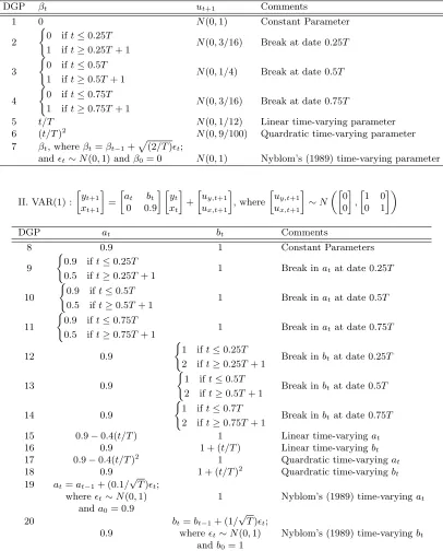
iden-tical normal distributions. The regressor in Model I is simply a vector of ones. Detailed setups for these two types of DGPs are listed in Table 2.1. DGPs 1 to 7 are based on Model I. DGPs 8 to 20 are based on Model II, which is the bivariate VAR(1) model used in Pesaran and Timmermann’s (2007) Monte Carlo simulations.
parameters with one break; (3) smooth time-varying parameters; and (4) Nyblom’s (1989) random walk parameter model. First, constant parameters are used in DGP 1 and 8. Second, DGPs from 2 through 4 and 9 through 14 consider parameters with a one-time break: the break date is 0.25T for DGP 2, 9 and 12, 0.5T for DGP 3, 10 and 13, 0.75T for DGP 4, 11 and 14, respectively. Third, DGPs from 5 through 6 and 15 through 18 use smooth time-varying parameters: in DGP 5, 15 and 16, parameters are linear functions of t; in DGP 6, 17 and 18, parameter functions are quadratic in t. Fourth, Nyblom’s random walk parameter is used in DGPs 7, 19 and 20.
Note that in DGP 2, 3 and 4, the variance of error term is chosen by equalizing the variance of {βt} and the variance of {ut+1} for each break date. In DGP 7, the variance of the error
term of the random coefficient βt is controlled so that the variance of the random coefficients
equals the variance of the error term of the model. DGPs 8 through 20 generate the process
{yt+1}using the VAR(1) model, eq. (1.9). In this experiment, the goal is to predictyT+1.yt+1
is regressed on its lagged value and xt, which itself follows AR(1). The parameter associated
with the lagged dependent variable, at, is less than one to ensure stability. DGPs 19 and 20
consider random walk processes in at and bt, respectively. The variances of the error term in
random coefficients are assumed to be relatively small so that the parameters change smoothly.
1.3.2 Window Selection Methods
The window selection methods implemented in Table 1.3 and Table 1.4 include: (i) five methods used in Pesaran and Timmermann (2007), PT hereafter; (ii) Cai’s AIC bandwidth selection rule (Cai, 2007); (iii) our proposed window selection method based on the approximate MSFE de-signed for models with smooth time-varying parameters; and (iv) our proposed window selection method based on the infeasible MSFE.
methods when the parameters are smoothly time-varying.
Second, Cai’s (2007) AIC bandwidth selection method is to choose a bandwidth, denoted by τ using notations in Cai (2007), to minimize
AIC(τ) = log(ˆσ2) + 2(nτ + 1)/(n−nτ−2), (1.10)
where n is the sample size, ˆσ2 = (1/n)Pn
t=1(yt−yˆt)2 and nτ is the trace of the matrix Hτ.
Here Hτ satisfies ˆY = HτY, where Y = (y1,· · · , yn)0. We refer the interested reader to Cai
(2007) for details. Note that the product of the sample sizenand the bandwidthτ,nτ, equals the window sizeR in this chapter. It is also important to note that Cai’s bandwidth selection method was not designed to produce the best forecasts for the future. The AIC criterion in eq. (1.10) is based on the sum of the squared estimated errors of all the forecasts from time 1 through time T. Thus for models with smooth time-varying parameters, Cai’s AIC method is expected to be worse than our new window selection method when the objective is to minimize the MSFE of forecast ˆyT+1. In Cai’s AIC method, the optimal window is searched from 0.2T
to 0.7T at a step size equal to 0.025T.
Third, the window selection method developed in this chapter is implemented as follows: Step (1): Test whether the parameters are constant using the test in Bai and Perron (1998, Section 4.1). Critical values are set at the 5% significance level. The trimming range for the possible break dates is [0.15T,0.85T].
Step (2): If we fail to reject the null hypothesis of constant parameters in Step (1), set the optimal window R to the full sample size. Otherwise, setR0 = 1.2T4/5,R = max(2T3/5,0.2T)
and ¯R = min(2T4/5,0.8T), then select window R from (R,R¯) to minimize the approximate conditional MSFE ( ˆβR(1)−β˜(1))0xTx0T( ˆβR(1)−β˜(1)).
Fourth, the infeasible window selection criterion ( ˆβR(1)−β(1))0xTx0T( ˆβR(1)−β(1)) is also
considered. Here R is chosen in the range [0.1T,0.9T]. This infeasible version, which uses the true value of β(1) instead of the estimated value ˜β(1), should always perform better than our approximate MSFE criterion.
1.3.3 Simulation Results
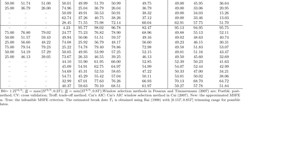
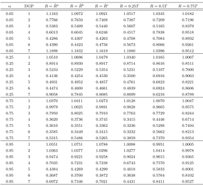
The main findings are summarized in Tables 1.3, 1.4, 1.5 and 1.6, which are based on 5,000 Monte Carlo replications with sample size T=100 and T=200. Tables 1.3 and 1.4 report the ratios of the RMSFEs (square root MSFEs) produced by the optimal window size relative to the RMSFEs produced in the full sample:
v u u t
P5,000 m=1(y
(m) T+1−yˆ
(m) T+1)2 P5,000
m=1(y (m) T+1−y˜
(m) T+1)2
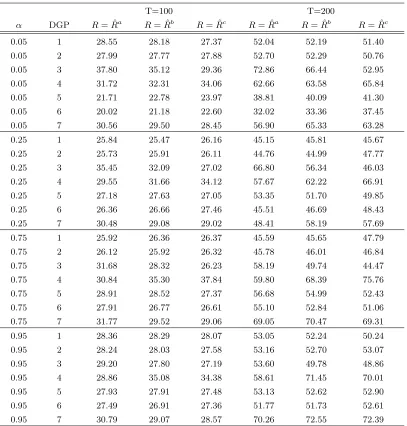
where ˆy(m)T+1 is the forecast computed using the optimal window size obtained using the window selection methods for the mth replication and ˜yT(m)+1 is the forecast computed using the full sample for the mth replication. The benchmark forecast, based on the full sample, should perform the best for models with constant parameters. If the relative root MSFE given in eq. (1.11) is less than one, the forecast estimated using the window size chosen by the window selection methods performs better than the benchmark forecast. Tables 1.5 and 1.6 report the average of the window sizes chosen by the window selection methods over the 5,000 simulations. The average window sizes shown in Tables 1.5 and 1.6 suggest that when parameters are constant, all window selection methods tend to choose large estimation sizes. The average window sizes are close to the full sample size. When DGPs have sharp breaks, except Cai’s AIC method, the averages of the window sizes chosen by the other methods tend to decrease as the break dates get closer to the end of the sample.
The results of the relative MSFEs in Tables 1.3, 1.4, suggest the following conclusions. First, the infeasible MSFE criterion (in column “True”) produces the smallest relative RMS-FEs in all DGPs. Also, asT increases, all the relative RMSFEs produced by the infeasible MSFE criterion become smaller in all the experiments. It was expected that the infeasible MSFE cri-terion has a good performance for models with smoothly time-varying parameters, because it is designed for this kind of models and the true value of the parameterβ(1) is used. It is surprising that this infeasible MSFE criterion also works very well for models with a one-time discrete break and Nyblom’s random walk parameter model.
Second, for the models with smooth time-varying parameters simulated in DGPs 5 through 6 and 15 through 18, the approximate MSFE criterion (in column “New”) yields the seond smallest relative RMSFEs forT = 100,200. It is natural for the approximate MSFE criterion to perform worse than the infeasible MSFE criterion, because replacingβ(1) with the local linear estimates ˜β(1) introduces additional noise into the MSFE criterion. Except for the infeasible MSFE criterion, the approximate MSFE criterion can beat all the existing window selection methods that are not designed for models with smoothly time-varying parameters. The im-provement compared to the existing window selection methods is remarkable, and becomes more substantial the larger T is.
per-formance of the approximate MSFE criterion is comparable to PT’s window selection methods for T = 100,200. In other words, the relative RMSFEs produced by the approximate MSFE criterion is smaller than the worst method among the five methods of PT and close to the best method of PT. For instance, the post-break method (in column “Postbk”) and the trade-off method (in column “Troff”) perform the best among the five methods of PT. The relative root MSFEs of the approximate MSFE criterion are close to these two methods and get closer as T increases. It is also worth noting that Cai’s (2007) AIC method also performs well when the underlying models have one break. The approximate MSFE criterion performs worse than the AIC method in DGPs 2, 3 and 4 forT = 100, especially in DGP 4. However, as T increases to 200, the approximate MSFE criterion performs better than the AIC method in DGPs 2 and 4 and perform very close to the AIC method in DGP 3.
Fifth, for T = 200, the approximate MSFE criterion performs the second best in DGP 7, which simulates a univariate model with a time-varying parameter following a random walk process. The approximate MSFE criterion performs a little worse than Cai’s AIC method when T = 100, but turns to perform better than Cai’s AIC method as T increases. The approximate MSFE criterion works much better than the five methods of PT for bothT = 100 andT = 200. This result suggests that in the random walk model, even when random coefficient is not as smooth as in DGP 5 and 6, the approximate MSFE criterion still works.
Sixth, in DGPs 9 through 11, the performance of the approximate MSFE criterion is com-parable to PT. DGPs 9, 10 and 11 assume that at breaks at date 0.25T, 0.5T and 0.75T,
respectively. The relative RMSFEs produced by the five methods of PT are similar to the re-sults reported in Table 2 in PT. Among the methods they propose based on the estimated break date ˆT1, the cross validation method (in column “CV”) performs the best in DGPs 9 and 10
and the post-break method performs the best in DGP 11 for bothT = 100 andT = 200. This suggests that cross validation works better for models with early breaks and the post-break method works better for models with break dates close to the end of the sample. The rela-tive RMSFEs produced by the approximate MSFE criterion are larger than, but close to, the smallest relative root MSFEs produced by the five methods of PT. One exception is DGP 11 whenT = 100, in which the smallest relative RMSFE of the five methods in PT based on ˆT1 is
0.7069, whereas the relative RMSFE produced by the approximate MSFE criterion is 0.8178, relatively far from the smallest value. However, as T increases to 200, the relative RMSFE of the approximate MSFE criterion becomes close to the smallest relative RMSFE achieved by PT’s methods.
suggests that Cai’s AIC method works well for the process generated from a bivariate VAR(1) model with one break. The approximate MSFE criterion can beat Cai’s AIC method in large sample and models with break dates close to the end of the sample.
Eighth, in DGPs 12 to 14, for both T = 100 and T = 200, the post-break method performs the best among the five methods of PT. DGPs 12, 13 and 14 assume the parameter associated with the exogenous variable,bt, breaks at date 0.25T, 0.5T and 0.75T, respectively. This suggests
that the post-break method is effective for the instability caused by exogenous processes. The performance of the trade-off method is very close to the post-break method.
Ninth, in DGPs 12 to 14, the performance of the approximate MSFE criterion is worse than the post-break method forT = 100,200. Although the discrepancy becomes smaller asT increases. When the sample is large (T = 200) and breaks happen late in the sample (T1 =
0.75T), the approximate MSFE method performs almost as well as the post-break method. Tenth, DGP 12 shows that the approximate MSFE criterion performs worse than Cai’s AIC method for models with early break dates and DGP 14 shows that the approximate MSFE criterion performs better than Cai’s AIC method for models with late break dates. This suggests that Cai’s AIC method works well for breaks that happen early in the sample.
Eleventh, in DGP 19, without considering the infeasible MSFE criterion, the approximate MSFE criterion performs worse than the post-break method and better than all the rest of the methods when T = 100 and it performs the best among all the methods when T = 200. This pattern suggests that, as the sample size increases, the approximate MSFE criterion can lead to a window size that is optimal for forecasting when the parameter associated with the lagged dependent variable follows a random walk process. Note that the standard deviation of the error term in the process of the random coefficientatis set at a small value, 0.1/
√
T. The purpose of this setting is to prevent at from exceeding unity, in which case the process yt would explode
and become unstable. Simulations withatgreater than one are considered bad simulations thus
are discarded. By choosing a small variance of the error term in theat process, the number of
bad simulations is very small.
Twelfth, in DGP 20, the performance of the approximate MSFE criterion is the best among all the methods for T = 100,200, except of course that of the infeasible MSFE criterion. Here the change inbt associated with the exogenous variable would not give rise to unstable process
yt, so the standard deviation of the error term in bt is 1/ √
T, which is larger than that of at.
However, letting this variance decrease asT increases guarantees some degree of smoothness in the way the random coefficient changes.
ap-proximate MSFE criterion cannot beat the best existing window selection methods designed for discrete breaks, but is not worse than the worst existing methods proposed for discrete breaks.
1.4
Empirical Analysis
This section examines the practical value of the approximate conditional MSFE criterion devel-oped in Section 2.2. This new approach is applied to forecasting output growth and inflation a topic for which Stock and Watson (1999, 2003, 2007) provide a comprehensive literature review and empirical analysis. They find strong evidence of instability in predictive relations, which means that finding a predictor useful in one period does not guarantee that it will predict well in later periods. For instance, they find that forecasts of output growth based on the term spread, (that is, the long-term government bond rate minus the federal funds rate), improve upon a simple AR model from 1971 through 1984, but are worse than the AR forecasts for the post 1984 period. The main results reported in Stock and Watson (1999, 2003, 2007) are based on the recursive out-of-sample forecasting, which uses all the data available up to the time the forecast is made, although they also experiment with rolling out-of-sample forecasting using a fixed window size. The purpose of this section is to check whether we can improve forecasts of output growth and inflation using the window size chosen by our new approach.
1.4.1 Data
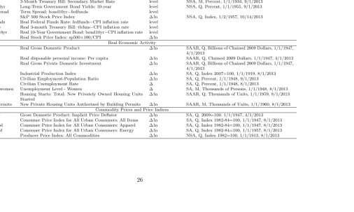
We use quarterly data to forecast output growth and inflation for the United States. Quarterly values of monthly series are computed by averaging monthly values over the three months in the quarter. We use the growth rate of the real GDP to measure output growth and the GDP deflator to measure inflation. The series of exogenous predictors, described in Table 1.7, are publicly available from the Federal Reserve Economic Data of the St. Louis Fed. Most of these predictors appear in Stock and Watson (2003, 2007). The exogenous predictors mainly consist of asset prices, measures of real economic activity, price indices and monetary measures. We interpret asset prices as including interest rates, differences between interest rates and the value of financial and tangible assets such as S&P 500 stock index and gold price.
1.4.2 Forecasting Models
The h-step ahead linear forecasting model for output growth is:
yt+hh =µt+αt(L)xt+βt(L)yt+ut+h, (1.12)
where the dependent variable isyh
t+h= (400/h) ln(Qt+h/Qt), xt denotes the exogenous
predic-tor,yt= 400 ln(Qt/Qt−1), and Qt denotes the quarterly real GDP in levels.
The h-step ahead linear forecasting model for inflation is:
πt+hh −πt=µt+αt(L)xt+βt(L)∆πt+ut+h, (1.13)
where πt = 400 ln(Pt/Pt−1), ∆πt =πt−πt−1, πht+h =h−1Phi=1πt+i, Pt is the quarterly GDP
deflator in levels, and xt is the exogenous predictor. Futthermore, αt(L)xt denotes the lag
polynomial.αt(L)xt=α1txt+α2txt−1+. . .+αptxt−p+1, andp is the number of lags. We refer
toxt as a lagged value because it is lagged relative to the dependent variable to be forecasted.
The same definition applies toβt(L)yt and βt(L)∆πt.
1.4.3 Results
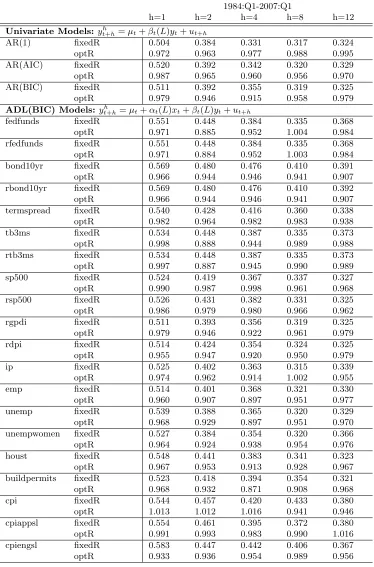
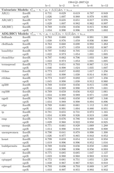
The results of the pseudo out-of-sample forecasting for output growth and inflation are summa-rized in Table 1.8 and Table 1.9, respectively. We consider two type of models: autoregressive (AR) models and autoregressive distributed lag (ADL) models, eq. (1.12) and eq. (1.13), re-spectively. In the AR model, only lagged values of the variable to be forecasted apprear as regressors. In the ADL model, regressors include an intercept term, the exogenous variablext
and the lagged dependent variable (yt for forecasting output growth or ∆πt for forecasting
inflation). We use ADL models to evaluate the predictive ability of the exogenous predictor in the presence of the lagged dependent variable as a regressor because, when the series to be forecasted is serially correlated, its own past values may be themselves useful predictors.
For each model in Tables 1.8 and 1.9, the first row reports the RMSFEs of h-step-ahead forecast when a fixed window of 40 observations is used (labeled “fixedR”) as in Stock and Watson (2001). The second row reports the relative RMSFEs of forecasts using the optimal window size chosen by the new approach to the values in the first row (labeled “optR”). If the value in the second row is less than one, it means that the optimal window size improves the forecast performance relative to the fixed window size.
focus on the BIC results because the BIC is a consistent estimator of the true lag length, and tends to select fewer lags than the AIC.
The results in Table 1.8 suggest the following conclusions for forecasting output growth. Overall, forecasts based on the optimal window sizes perform better than the fixed window size, for both AR and ADL models, especially when the forecast horizon is small. The improve-ment ranges from 1 percent to 12 percent. For AR models, the forecasting improveimprove-ment based on the optimal window sizes appears at one, two and four horizons. The AR model with the BIC lags has the best performance among three AR models. When we forecast two-quarter-ahead or four-quarter-two-quarter-ahead real GDP growth, the optimal window size procedure can reduce the RMSFEs by about 5 percent relative to the fixed window one.
In ADL models where the number of lags is chosen by the BIC, forecasts made by using the federal funds rate, the 10-year bond rate, the term spread and the 3-month treasury bill rate as predictors improve by about 5 percent when using the optimal window size procefure. These asset prices are useful in predicting output growth in part because they reveal expectations about the future state of the economy. Stock and Watson (2003) found that the term spread is useful for forecasting output growth, and they suspected parameter instabilities in the predictive relations. Our results support this conclusion, as our optimal window size procedure allows the model to select the best amount of past information to forecast at each point in time, and adapts it as time goes by.
When forecasting output growth with measures of real economic activity, the optimal win-dow size seems to improve forecasts for most models and most forecast horizons. Improvements appear in forecasts with real disposable personal income (rdpi), the number of housing starts (houst) and building permits (buildpermits) for privately owned housing. Especially, building permits contain significant predictive contents for two-quarter-ahead, four-quarter-ahead and eight-quarter-ahead output growth forecasts. Our interpretation is that building constructions typically take a long time to complete, so the number of building permits is an indicator of the economic activity far in the future. When the number of building permits increases, future investment in building constructions will increase and contribute to output growth. In addition, the optimal window size can improve forecasts made by price indices like CPI and PPI for most forecast horizons, and monetary measures such as M0, M1, and M2.
The results in Table 1.9 suggest the following conclusions for forecasting inflation.
models while they do not in inflation forecasts. The lack of varying parameters is one possible reason for the poor improvement of the optimal window size at short forecast horizons.
For forecasting models based on measures of economic activities, the long-term inflation forecasts perform better when optimal window sizes are used. Measures oof unemployment (emp, unemp and unempwomen) tend to be useful predictors for inflation when the optimal window size is used at most forecast horizons. The degree of improvement ranges from 5 percent to almost 11 percent. One possible explanation is that the non-accelerating inflation rate of unemployment (NAIRU) in the unemployment-based Phillips curve, which is modeled by the intercept term, may be unstable, and the optimal window size captures this time variation.
The empirical evidence on the usefulness of the optimal window size is mixed for inflation forecasts based on monetary measures. Forecasts based on the optimal window size using M0 as the predictors improve more than using other monetary measures.
1.5
Discussion and Conclusion
This chapter introduced a new approach to select the size of the rolling estimation window for pseudo out-of-sample forecasting. The forecasting models allow for parameter instability, which is described by smoothly time-varying parameters. The optimal window size minimizes the conditional mean squared forecast error of forecast made at the end of the sample. We have shown that the optimal window is of the order of magnitude T2/3. However, in real-time forecasting, forecasters do not know the actual value of the target variable in the future, therefore, we provided an approximate conditional MSFE criterion for window selection.
The approximate conditional MSFE criterion chooses a window sizeRto minimize ( ˆβR(1)−
˜
β(1))0xTx0T( ˆβR(1)−β˜(1)), where the models’ parameter estimate ˆβR(1), depends on R, and
˜
β(1), the proxy for the true parameter at the end of the sample β(1), is estimated by local linear regressions. Under certain conditions, which we studied in the chapter, the approximate conditional MSFE is asymptotically optimal with respect to the infeasible conditional MSFE criterion.
Monte Carlo simulations show that simple univariate and bivariate VAR(1) models, using the window size chosen by the approximate conditional MSFE criterion, improves the forecast-ing performance relative to usforecast-ing the full sample when the underlyforecast-ing model is generated by smoothly time-varying parameters and random parameters. For processes generated by param-eters with discrete breaks, the performance of the approximate conditional MSFE criterion is comparable to that of existing window selection methods designed for discrete breaks.
contain useful predictive content for forecasting output growth at short forecast horizons. When forecasting inflation, measures of unemployment are still useful, confirming the usefulness of the unemployment-based Phillips curve in the presence of the parameter instabilities. In gen-eral, the improvement at short forecast horizons, resulting from using our optimal window size procedure is more significant than forecasting output growth than inflation, since parameters are likely to vary in the former than in the latter case.
Some caveats are as follows. First, the new window selection method chooses a uniform window size for all the time-varying parameters. When parameters have different patterns of time variation, one window size may not be optimal for all the parameters. Thus for models with many predictors, the performance of the window selection method would deteriorate. We could improve upon existing results by choosing an optimal window for each time-varying parameter. Second, in practice, it is hard for forecasters to know whether the underlying model is subject to discrete breaks or smooth time variation. A careful forecaster should first compare the window selection methods for discrete breaks and the approximate conditional MSFE criterion developed in this chapter, and then determine the best window selection methods. Third, the choice of R0 affects the performance of the approximate conditional MSFE criterion. In the
proof of the asymptotic optimality of the new approach, the constant associated with the rate is not specified. When practitioners use our method in practice, they need to experiment on various constants to determine R0. Fourth, the model setup in this chapter does not allow
Table 1.2: Description of DGPs
I. Univariate case:yt+1=βt+ut+1
DGP βt ut+1 Comments
1 0 N(0,1) Constant Parameter
2
(
0 ift≤0.25T
1 ift≥0.25T+ 1 N(0,3/16) Break at date 0.25T
3
(
0 ift≤0.5T
1 ift≥0.5T+ 1 N(0,1/4) Break at date 0.5T
4
(
0 ift≤0.75T
1 ift≥0.75T+ 1 N(0,3/16) Break at date 0.75T
5 t/T N(0,1/12) Linear time-varying parameter 6 (t/T)2 N(0,9/100) Quardratic time-varying parameter
7 βt, whereβt=βt−1+ p
(2/T)t;
andt∼N(0,1) andβ0= 0 N(0,1) Nyblom’s (1989) time-varying parameter
II. VAR(1) :
yt+1
xt+1
=
at bt
0 0.9
yt
xt
+
uy,t+1
ux,t+1
, where
uy,t+1
ux,t+1
∼N
0 0
,
1 0 0 1
DGP at bt Comments
8 0.9 1 Constant Parameters
9
(
0.9 ift≤0.25T
0.5 ift≥0.25T+ 1 1 Break inat at date 0.25T 10
(
0.9 ift≤0.5T
0.5 ift≥0.5T+ 1 1 Break inat at date 0.5T 11
(
0.9 ift≤0.75T
0.5 ift≥0.75T+ 1 1 Break inat at date 0.75T
12 0.9
(
1 ift≤0.25T
2 ift≥0.25T+ 1 Break inbt at date 0.25T
13 0.9
(
1 ift≤0.5T
2 ift≥0.5T+ 1 Break inbt at date 0.5T
14 0.9
(
1 ift≤0.7T
2 ift≥0.75T+ 1 Break inbt at date 0.75T 15 0.9−0.4(t/T) 1 Linear time-varyingat
16 0.9 1 + (t/T) Linear time-varyingbt
17 0.9−0.4(t/T)2 1 Quardratic time-varyingat
18 0.9 1 + (t/T)2 Quardratic time-varyingbt
19 at=at−1+ (0.1/ √
T)t;
wheret∼N(0,1) 1 Nyblom’s (1989) time-varyingat
anda0= 0.9
20 bt=bt−1+ (1/
√
T)t;
0.9 wheret∼N(0,1) Nyblom’s (1989) time-varyingbt
Table 1.3: Root MSFE (T=100)
known break date (infeasible) Estimated break date ( ˆT1) unknown break date Cai’s
DGP Postbk CV WA Pooled Troff Postbk CV WA Pooled Troff CV WA Pooled AIC New True 1 – – – – – 1.0005 1.0001 1.0000 1.0000 1.0005 1.0068 1.0016 1.0039 1.0067 1.0015 0.9999 2 0.8731 0.8799 0.9158 0.9106 0.8731 0.8736 0.8801 0.9159 0.9108 0.8736 0.8830 0.8809 0.8784 0.8901 0.8850 0.8671 3 0.7186 0.7219 0.8591 0.8315 0.7186 0.7183 0.7221 0.8591 0.8314 0.7183 0.7231 0.8229 0.7551 0.7313 0.7338 0.7105 4 0.5151 0.6248 0.8746 0.7991 0.5151 0.5151 0.6248 0.8746 0.7992 0.5151 0.6248 0.8746 0.7272 0.5237 0.5831 0.5047 5 – – – – – 0.6605 0.6530 0.8488 0.8208 0.6605 0.5986 0.8129 0.6976 0.7067 0.5835 0.5223 6 – – – – – 0.6013 0.6204 0.8602 0.8176 0.6013 0.6015 0.8499 0.7186 0.6148 0.5782 0.4470 7 – – – – – 0.8878 0.8905 0.9502 0.9365 0.8878 0.8733 0.9382 0.8935 0.8690 0.8717 0.8188 8 – – – – – 1.0183 1.0040 1.0005 1.0006 1.0176 1.0175 1.0110 1.0188 1.0264 1.0137 0.9988 9 0.8034 0.7959 0.9386 0.9237 0.8061 0.8060 0.7969 0.9393 0.9245 0.8082 0.8042 0.8305 0.8060 0.8243 0.8328 0.7724 10 0.7134 0.6963 0.9248 0.9032 0.7207 0.7147 0.6966 0.9250 0.9034 0.7217 0.7009 0.8718 0.7634 0.7332 0.7335 0.6679 11 0.7038 0.9088 0.9491 0.9100 0.7444 0.7069 0.9091 0.9494 0.9124 0.7463 0.9088 0.9491 0.8392 0.8053 0.8178 0.6127 12 0.8795 0.8837 0.9387 0.9284 0.8812 0.8810 0.8846 0.9376 0.9274 0.8827 0.8933 0.8924 0.8908 0.9233 0.9254 0.8568 13 0.7305 0.7337 0.8895 0.8604 0.7394 0.7315 0.7346 0.8895 0.8602 0.7415 0.7382 0.8494 0.7726 0.7843 0.7697 0.6963 14 0.6429 0.7844 0.8936 0.8285 0.6692 0.6514 0.7854 0.8945 0.8316 0.6747 0.7844 0.8936 0.7724 0.7543 0.7014 0.5835 15 – – – – – 0.8471 0.8467 0.9264 0.9148 0.8490 0.8301 0.8924 0.8445 0.8696 0.8239 0.7661 16 – – – – – 0.8504 0.8474 0.9151 0.9020 0.8517 0.8299 0.8843 0.8386 0.8640 0.8300 0.7611 17 – – – – – 0.7978 0.8087 0.9213 0.9017 0.8017 0.7918 0.9012 0.8222 0.8560 0.7583 0.6767 18 – – – – – 0.7785 0.7897 0.9012 0.8749 0.7835 0.7752 0.8813 0.8020 0.8424 0.7533 0.6650 19 – – – – – 0.9731 0.9997 0.9939 0.9908 0.9999 0.9996 0.9938 0.9891 0.9893 0.9817 0.9399 20 – – – – – 0.8316 0.8381 0.9290 0.9012 0.8357 0.8292 0.9119 0.8352 0.8467 0.8139 0.7059 Notes: R0= 1.2T4/5;R= max(2T3/5,0.2T); R= min(2T4/5,0.8T); Five window selection methods in Pesaran and Timmermann (2007) are: (1)Postbk:
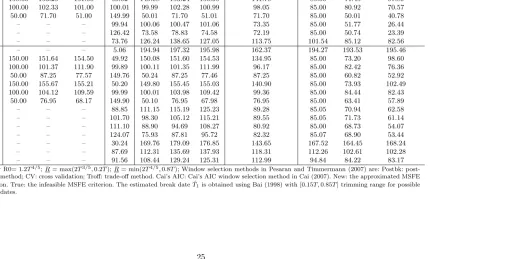
Table 1.4: Root MSFE (T=200)
known break date (infeasible) Estimated break date ( ˆT1) unknown break date Cai’s
DGP Postbk CV WA Pooled Troff Postbk CV WA Pooled Troff CV WA Pooled AIC New True 1 – – – – – 1.0004 1.0000 0.9999 1.0000 1.0004 1.0032 1.0007 1.0013 1.0038 1.0006 0.9998 2 0.8660 0.8690 0.9134 0.9081 0.8660 0.8662 0.8691 0.9135 0.9082 0.8662 0.8705 0.8753 0.8704 0.8743 0.8737 0.8641 3 0.7088 0.7105 0.8573 0.8298 0.7088 0.7091 0.7106 0.8573 0.8298 0.7091 0.7110 0.8191 0.7487 0.7140 0.7172 0.7055 4 0.5043 0.6112 0.8720 0.7982 0.5043 0.5043 0.6112 0.8720 0.7983 0.5043 0.6112 0.8720 0.7231 0.5058 0.5037 0.4995 5 – – – – – 0.6571 0.6522 0.8464 0.8204 0.6571 0.5901 0.8102 0.6937 0.7067 0.5478 0.5113 6 – – – – – 0.5966 0.6138 0.8569 0.8170 0.5966 0.5954 0.8481 0.7161 0.5468 0.5185 0.4362 7 – – – – – 0.8645 0.8762 0.9464 0.9310 0.8644 0.8677 0.9378 0.8931 0.8526 0.8482 0.8058 8 – – – – – 1.0051 1.0006 0.9998 0.9997 1.0044 1.0052 1.0014 1.0046 1.0067 1.0035 0.9998 9 0.7494 0.7436 0.9232 0.9044 0.7504 0.7496 0.7437 0.9235 0.9047 0.7505 0.7477 0.7914 0.7552 0.7649 0.7655 0.7376 10 0.6696 0.6630 0.9142 0.8912 0.6715 0.6697 0.6629 0.9143 0.8914 0.6717 0.6639 0.8586 0.7362 0.6772 0.6903 0.6538 11 0.6243 0.8330 0.9361 0.8925 0.6342 0.6250 0.8330 0.9362 0.8931 0.6351 0.8330 0.9361 0.8140 0.6586 0.6342 0.5952 12 0.8578 0.8605 0.9226 0.9120 0.8585 0.8577 0.8607 0.9225 0.9120 0.8583 0.8632 0.8723 0.8644 0.8840 0.8873 0.8513 13 0.6855 0.6879 0.8685 0.8349 0.6887 0.6853 0.6875 0.8682 0.8345 0.6886 0.6886 0.8266 0.7361 0.7069 0.7140 0.6764 14 0.5663 0.7071 0.8909 0.8210 0.5755 0.5666 0.7071 0.8909 0.8212 0.5760 0.7071 0.8909 0.7529 0.6008 0.5792 0.5453 15 – – – – – 0.8125 0.8092 0.9123 0.9010 0.8155 0.7748 0.8705 0.8124 0.8379 0.7655 0.7357 16 – – – – – 0.7803 0.7810 0.8932 0.8785 0.7827 0.7618 0.8650 0.8025 0.8353 0.7439 0.7050 17 – – – – – 0.7686 0.7678 0.9108 0.8927 0.7729 0.7389 0.8902 0.8016 0.8019 0.6953 0.6541 18 – – – – – 0.7058 0.7224 0.8845 0.8553 0.7086 0.7121 0.8725 0.7780 0.8031 0.6599 0.6061 19 – – – – – 0.9408 0.9483 0.9873 0.9838 1.0000 0.9483 0.9873 0.9684 0.9390 0.9283 0.8555 20 – – – – – 0.8030 0.8135 0.9264 0.8973 0.8053 0.8042 0.9102 0.8278 0.7873 0.7638 0.6813 Notes: R0= 1.2T4/5;R= max(2T3/5,0.2T); R= min(2T4/5,0.8T); Five window selection methods in Pesaran and Timmermann (2007) are: (1)Postbk:
Table 1.5: Average Window Size Across Monte Carlo Replications (T=100)
known break date (infeasible) estimated break date ( ˆT1) unknown break date
DGP Postbk CV Troff Tˆ1 Postbk CV Troff CV Cai’s AIC New True
1 – – – 0.23 99.77 99.84 99.77 79.67 98.20 98.01 98.69
2 75.00 77.43 76.00 25.00 75.00 77.42 76.00 71.69 49.00 54.26 50.77
3 50.00 51.74 51.00 50.01 49.99 51.70 50.99 49.75 49.00 45.95 36.64
4 25.00 36.79 26.00 74.96 25.04 36.79 26.04 36.79 49.00 33.06 20.95
5 – – – 50.09 49.91 50.53 50.91 38.32 49.00 34.03 15.26
6 – – – 62.74 37.26 40.75 38.26 37.12 49.00 33.46 13.03
7 – – – 28.45 71.55 75.98 72.14 60.04 62.91 57.75 51.70
8 – – – 4.23 95.77 98.02 96.78 82.47 95.13 94.95 95.75
9 75.00 76.80 79.02 24.77 75.23 76.82 78.90 68.96 49.88 55.13 52.11
10 50.00 51.57 59.43 49.94 50.06 51.51 59.57 49.16 49.02 48.63 40.74
11 25.00 56.60 48.22 74.08 25.92 56.79 48.17 56.60 49.23 46.15 30.31
12 75.00 79.54 79.23 25.22 74.78 79.40 78.86 72.98 49.58 51.83 53.07
13 50.00 54.19 57.29 50.05 49.95 53.99 57.25 52.15 49.01 51.16 43.47
14 25.00 46.13 39.05 73.67 26.33 46.55 39.25 46.13 49.50 45.60 32.69
15 – – – 44.10 55.90 61.95 66.00 52.85 52.39 50.23 41.63
16 – – – 45.09 54.91 62.75 64.97 54.99 54.07 52.44 42.99
17 – – – 54.69 45.31 52.53 58.65 47.22 50.33 47.00 34.21
18 – – – 54.71 45.29 55.42 57.04 50.11 53.01 50.02 38.06
19 – – – 32.99 67.01 77.63 76.26 66.93 70.13 68.70 64.72
20 – – – 40.37 59.63 70.10 68.51 61.97 59.27 57.78 51.84
Notes: R0= 1.2T4/5;R= max(2T3/5,0.2T);R= min(2T4/5,0.8T);Window selection methods in Pesaran and Timmermann (2007) are: Postbk:
post-break method; CV: cross validation; Troff: trade-off method. Cai’s AIC: Cai’s AIC window selection method in Cai (2007). New: the approximated MSFE criterion. True: the infeasible MSFE criterion. The estimated break date ˆT1 is obtained using Bai (1998) with [0.15T ,0.85T] trimming range for possible
Table 1.6: Average Window Size Across Monte Carlo Replications (T=200)
known break date (infeasible) estimated break date ( ˆT1) unknown break date
DGP Postbk CV Troff Tˆ1 Postbk CV Troff CV Cai’s AIC New True
1 – – – 0.26 199.74 199.85 199.74 160.87 196.21 195.74 197.33
2 150.00 153.25 151.00 50.02 149.98 153.24 150.98 141.79 85.00 71.45 97.89
3 100.00 102.33 101.00 100.01 99.99 102.28 100.99 98.05 85.00 80.92 70.57
4 50.00 71.70 51.00 149.99 50.01 71.70 51.01 71.70 85.00 50.01 40.78
5 – – – 99.94 100.06 100.47 101.06 73.35 85.00 51.77 26.44
6 – – – 126.42 73.58 78.83 74.58 72.19 85.00 50.74 23.39
7 – – – 73.76 126.24 138.65 127.05 113.75 101.54 85.12 82.56
8 – – – 5.06 194.94 197.32 195.98 162.37 194.27 193.53 195.46
9 150.00 151.64 154.50 49.92 150.08 151.60 154.53 134.95 85.00 73.20 98.60
10 100.00 101.37 111.90 99.89 100.11 101.35 111.99 96.17 85.00 82.42 76.36
11 50.00 87.25 77.57 149.76 50.24 87.25 77.46 87.25 85.00 60.82 52.92
12 150.00 155.67 155.21 50.20 149.80 155.45 155.03 140.90 85.00 73.93 102.49
13 100.00 104.12 109.59 99.99 100.01 103.98 109.42 99.36 85.00 84.44 82.43
14 50.00 76.95 68.17 149.90 50.10 76.95 67.98 76.95 85.00 63.41 57.89
15 – – – 88.85 111.15 115.19 125.23 89.28 85.05 70.94 62.58
16 – – – 101.70 98.30 105.12 115.21 89.55 85.05 71.73 61.14
17 – – – 111.10 88.90 94.69 108.27 80.92 85.00 68.73 54.07
18 – – – 124.07 75.93 87.81 95.72 82.32 85.07 68.90 53.44
19 – – – 30.24 169.76 179.09 176.85 143.65 167.52 164.45 168.24
19 – – – 87.69 112.31 135.69 137.93 118.31 112.26 102.61 102.28
20 – – – 91.56 108.44 129.24 125.31 112.99 94.84 84.22 83.17
Notes: R0= 1.2T4/5;R= max(2T3/5,0.2T); R= min(2T4/5,0.8T); Window selection methods in Pesaran and Timmermann (2007) are: Postbk:
post-break method; CV: cross validation; Troff: trade-off method. Cai’s AIC: Cai’s AIC window selection method in Cai (2007). New: the approximated MSFE criterion. True: the infeasible MSFE criterion. The estimated break date ˆT1 is obtained using Bai (1998) with [0.15T ,0.85T] trimming range for possible
Table 1.7: Data Description
Mnemonics Description Transformation Other Information: Seasonal Adjustment, Frequency, Units, Start Date, End Date
Asset Prices
fedfunds Effective Federal Funds Rate level NSA, M, Percent, 7/1/1954, 9/1/2013 tb3ms 3-Month Treasury Bill: Secondary Market Rate level NSA, M, Percent, 1/1/1934, 9/1/2013 bond10yr Long-Term Government Bond Yields: 10-year level NSA, Q, Percent, 1/1/1955, 9/1/2013 termspread Term Spread: bond10yr−fedfunds level
sp500 S&P 500 Stock Price Index ∆ ln NSA, Q, Index, 1/2/1957, 10/14/2013 rfedfunds Real Federal Funds Rate: fedfunds−CPI inflation rate level
rtb3ms Real 3-month Treasury Bill: tb3ms−CPI inflation rate level rbond10yr Real 10-Year Government Bond: bond10yr−CPI inflation rate level rsp500 Real Stock Price Index: sp500×100/CPI ∆ ln Real Economic Activity
rgdp Real Gross Domestic Product ∆ ln SAAR, Q, Billions of Chained 2009 Dollars, 1/1/1947, 4/1/2013
rdpi Real disposable personal income: Per capita ∆ ln SAAR, Q, Chained 2009 Dollars, 1/1/1947, 4/1/2013 rgpdi Real Gross Private Domestic Investment ∆ ln SAAR, Q, Billions of Chained 2009 Dollars, 1/1/1947,
4/1/2013
ip Industrial Production Index ∆ ln SA, Q, Index 2007=100, 1/1/1919, 8/1/2013 emp Civilian Employment-Population Ratio ∆ ln SA, Q, Percent, 1/1/1948, 9/1/2013 unemp Civilian Unemployment Rate ∆ SA, Q, Percent, 1/1/1948, 8/1/2013
unempwomen Unemployment Level - Women ∆ SA, M, Thousands of Persons, 1/1/1948, 8/1/2013 houst Housing Starts: Total: New Privately Owned Housing Units
Started
∆ ln SAAR, Q, Thousands of Units, 1/1/1959, 8/1/2013 buildpermits New Private Housing Units Authorized by Building Permits ∆ ln SAAR, M, Thousands of Units, 1/1/1960, 8/1/2013
Commodity Prices and Price Indices
gdpdef Gross Domestic Product: Implicit Price Deflator ∆ ln SA, Q, 2009=100, 1/1/1947, 4/1/2013
Table 1.7: Continued
Mnemonics Description Transformation Other Information: Seasonal Adjustment, Frequency, Units, Start Date, End Date
Monetary Measure
m0 St. Louis Adjusted Monetary Base ∆ ln SA, M, Billions of Dollars, 1/1/1918, 9/1/2013 m1 M1 for United States ∆ ln SA, Q, Billions of Dollars, 1/1/1959, 8/1/2013 m2 M2 for United States ∆ ln NSA, Q, Billions of Dollars, 1/1/1959, 8/1/2013 m3 M3 for United States ∆ ln SA, Q, Billions of Dollars, 1/1/1959, 8/1/2013 rm0 Real M0: M0×100/CPI ∆ ln
rm1 Real M1: M1×100/CPI ∆ ln rm2 Real M2: M2×100/CPI ∆ ln rm3 Real M3: M3×100/CPI ∆ ln
Notes: The following abbreviations appear in the table: SA: seasonally adjusted; NSA: not seasonally adjusted; SAAR: seasonally adjusted at an annual rate; Q: quarterly; M: monthly. Let St denote the original series and Xt denote the series used in regressions.
The transformations are: (1) level:Xt=St; (2) ∆ ln:Xt= lnSt−lnSt−1; (3)∆:Xt=St−St−1. Series that are not seasonally adjusted
Table 1.8: Pseudo Rolling Out-of-Sample Forecasts of the Real GDP Growth Rate .
1984:Q1-2007:Q1
h=1 h=2 h=4 h=8 h=12
Univariate Models:yh
t+h=µt+βt(L)yt+ut+h
AR(1) fixedR 0.504 0.384 0.331 0.317 0.324
optR 0.972 0.963 0.977 0.988 0.995
AR(AIC) fixedR 0.520 0.392 0.342 0.320 0.329
optR 0.987 0.965 0.960 0.956 0.970
AR(BIC) fixedR 0.511 0.392 0.355 0.319 0.325
optR 0.979 0.946 0.915 0.958 0.979
ADL(BIC) Models:yht+h=µt+αt(L)xt+βt(L)yt+ut+h
fedfunds fixedR 0.551 0.448 0.384 0.335 0.368
optR 0.971 0.885 0.952 1.004 0.984
rfedfunds fixedR 0.551 0.448 0.384 0.335 0.368
optR 0.971 0.884 0.952 1.003 0.984
bond10yr fixedR 0.569 0.480 0.476 0.410 0.391
optR 0.966 0.944 0.946 0.941 0.907
rbond10yr fixedR 0.569 0.480 0.476 0.410 0.392
optR 0.966 0.944 0.946 0.941 0.907
termspread fixedR 0.540 0.428 0.416 0.360 0.338
optR 0.982 0.964 0.982 0.983 0.938
tb3ms fixedR 0.534 0.448 0.387 0.335 0.373
optR 0.998 0.888 0.944 0.989 0.988
rtb3ms fixedR 0.534 0.448 0.387 0.335 0.373
optR 0.997 0.887 0.945 0.990 0.989
sp500 fixedR 0.524 0.419 0.367 0.337 0.327
optR 0.990 0.987 0.998 0.961 0.968
rsp500 fixedR 0.526 0.431 0.382 0.331 0.325
optR 0.986 0.979 0.980 0.966 0.962
rgpdi fixedR 0.511 0.393 0.356 0.319 0.325
optR 0.979 0.946 0.922 0.961 0.979
rdpi fixedR 0.514 0.424 0.354 0.324 0.325
optR 0.955 0.947 0.920 0.950 0.979
ip fixedR 0.525 0.402 0.363 0.315 0.339
optR 0.974 0.962 0.914 1.002 0.955
emp fixedR 0.514 0.401 0.368 0.321 0.330
optR 0.960 0.907 0.897 0.951 0.977
unemp fixedR 0.539 0.388 0.365 0.320 0.329
optR 0.968 0.929 0.897 0.951 0.970
unempwomen fixedR 0.527 0.384 0.354 0.320 0.366
optR 0.964 0.924 0.938 0.954 0.976
houst fixedR 0.548 0.441 0.383 0.341 0.323
optR 0.967 0.953 0.913 0.928 0.967
buildpermits fixedR 0.523 0.418 0.394 0.354 0.321
optR 0.968 0.932 0.871 0.908 0.968
cpi fixedR 0.544 0.457 0.420 0.433 0.380
optR 1.013 1.012 1.016 0.941 0.946
cpiappsl fixedR 0.554 0.461 0.395 0.372 0.380
optR 0.991 0.993 0.983 0.990 1.016
cpiengsl fixedR 0.583 0.447 0.442 0.406 0.367