Abstract
KWAK, JAEWOOK. Delay Efficient CSMA Scheduling in Wireless Networks. (Under the direction of Dr. Do Young Eun.)
Scheduling or Media Access Control (MAC) algorithms in wireless communication networks play a central role in achieving efficient utilization of wireless resources and providing satisfac-tory quality-of-service. Designing such good scheduling algorithms is, however, a challenging task, as users in wireless networks may experience a complicated contention relationship among the participants. Recently, Glauber dynamics model has been used as a powerful tool to analyze and design CSMA type scheduling algorithms. These algorithms are computationally simple, inherently distributed, and also suitably designed for queue-based schemes providing the capa-bility to achieve the maximum throughput performance. However, the delay performance of these algorithms is often reported to be far from satisfactory, mainly due to the specific type of link activation rules that can be modeled as a Markov chain, imposes a fundamental constraint on how the link state can evolve over time. In this dissertation, we take a new approach to overcome the constraint so as to improving its delay performance.
In the first part of our approach, we propose a new algorithm, named delayed CSMA that can significantly improve the delay performance without imposing much difficulty for imple-mentation. The key idea is to utilize past state information observed by local link and then constructing a high-order Markov chain for the evolution of the feasible link schedules. In effect, the proposed algorithm virtually emulates having multiple instances of independent schedulers and alternate amongst them in a round-robin fashion. We show in theory and simulation that the proposed algorithm achieves the maximal throughput, and also provides much better delay performance by effectively “de-correlating” the link state process, and thereby resolves starvation of link service.
more skillfully manipulate the driving sequences of random variables that govern the evolution of schedule instances, such that the multiple instances of virtual schedulers become “negatively correlated” as oppose to having them run independently. As a result, this contributes to faster change of the link state, rendering it more like a periodic process and thus leading to better queueing performance.
Delay Efficient CSMA Scheduling in Wireless Networks
by Jaewook Kwak
A dissertation submitted to the Graduate Faculty of North Carolina State University
in partial fulfillment of the requirements for the Degree of
Doctor of Philosophy
Electrical and Computer Engineering
Raleigh, North Carolina
2016
APPROVED BY:
Mihail L. Sichitiu Wenye Wang
Harry G. Perros Do Young Eun
Dedication
Biography
Acknowledgements
Foremost, I would like to thank my advisor Dr. Do Young Eun. As my supervisor, he has advised me with enthusiasm during the entire years of my Ph.D. study. The relentless passion and desire for research he has shown to me have been great stimuli to pursue my research goal and grow myself as a research scientist. Without his help, I would not have been able to complete my study successfully.
Beside my advisor, I would like to thank my committee members, Dr. Harry G. Perros, Dr. Mihail L. Sichitiu, and Dr. Wenye Wang for their insightful comments and encouragement. Their hard questions provided me to contemplate my research from wider perspectives.
I also would like to give my thanks to all the former and current lab-mates: Sungwon Kim, Chul-Ho Lee, Xin Xu, Cindy Xu, and Honggyu Jung. I am in particular very grateful to Dr. Chul-Ho Lee for his insightful discussions and contributions to my research. And, I am so happy to have been able to share most of my Ph.D. life with Xin Xu.
Table of Contents
List of Tables . . . vii
List of Figures . . . .viii
Chapter 1 Introduction . . . 1
1.1 Related Work . . . 3
1.2 Contributions . . . 5
1.2.1 Identifying the correlation structure of link service process . . . 5
1.2.2 A New Scheduling Algorithm under a High-Order Markov Chain Model . 6 1.2.3 An Antithetic Coupling Approach to the CSMA Scheduling . . . 7
1.3 Organization . . . 8
Chapter 2 Preliminaries . . . 10
2.1 Network Model . . . 10
2.2 CSMA Scheduling as a Glauber Dynamics . . . 13
Chapter 3 Correlation Structure of the Standard CSMA . . . 17
3.1 Non-negativity of correlations over any time scale . . . 18
3.2 Quantifying the degree of correlations . . . 23
Chapter 4 CSMA Scheduling with High-Order Markov Chain Model . . . 27
4.1 Delayed CSMA . . . 28
4.2 Delay Performance . . . 33
4.3 Throughput Optimality . . . 38
4.4 Impact on Transient Behavior . . . 40
Chapter 5 Improving the Delay Performance via an Antithetic Coupling Ap-proach . . . 45
5.1 Antithetic coupling . . . 46
5.2 Generation of NA random variables . . . 48
5.3 Proposed algorithm: AC-CSMA . . . 49
5.4 Analysis on the Performance Improvement . . . 53
Chapter 6 Numerical Evaluation . . . 60
6.1 Delayed CSMA . . . 60
6.2 AC-CSMA . . . 68
Chapter 7 Conclusion . . . 74
References. . . 76
APPENDIX . . . 81
List of Tables
List of Figures
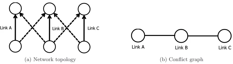
Figure 2.1 An instance of network topology with three communication links and its conflict graph. (a) Solid line indicates communication links to be used data transmission and dotted line represents interference caused to other communication links. (b) Each node represents corresponding communi-cation link and edge represents conflict relationship. . . 11 Figure 2.2 Capacity region of link arrival rates in the network topology given in
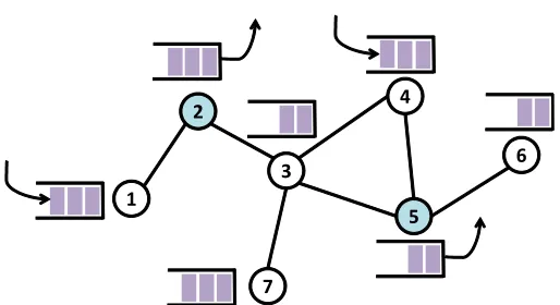
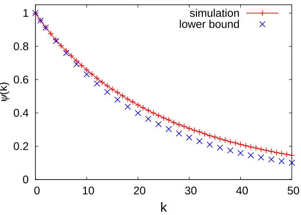
Figure 2.1 . . . 12 Figure 3.1 An instance of conflict graph with seven communication links. . . 25 Figure 3.2 Correlations of σ3(t) for the network in Figure 3.1 from simulations and
the lower bounds. . . 26 Figure 4.1 Comparison between the conventional CSMA and our proposed approach.
A box indicates a schedule, and arrows indicate state transitions. . . 28 Figure 4.2 Two properties of the algorithm: correlation-lag shifting and zero-correlation
padding . . . 33 Figure 4.3 Our algorithm has an effect of dividing the original net-input process of a
single stream (top) into a sum of i.i.d.substreams (bottom) in the steady state. . . 36 Figure 4.4 An illustration of the gentler start-up algorithm. Blue arrows indicate
state transitions. The algorithm starts att0withT initially sampled states. 42
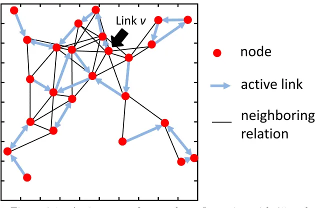
Figure 5.1 An instance of channel state where link vcan update its activities for the time slots t= 2 and 3. . . 50 Figure 6.1 An instance of network configuration with 25 nodes . . . 61 Figure 6.2 Mean and CoV of ‘off’ duration for σv(t) . . . 62
Figure 6.3 Histogram of At−St and its approximation by a Gaussian process. The
lines are Gaussian distribution drawn from measured sample mean and variance. . . 62 Figure 6.4 Delay performance of the delayed CSMA with various T under dynamic
fugacity . . . 64 Figure 6.5 Impact of T on a queue evolution. . . 66 Figure 6.6 Impact of M on (a) queue-length evolution and (b) correlation reduction . 67 Figure 6.7 Simulation topologies . . . 68 Figure 6.8 Correlations of service process measured at the designated node in the
Random network. . . 70 Figure 6.9 Normalized ratio of average queuing delay for each topology type as traffic
intensity varies. The parameterT = 2 is used for delayed CSMA and AC-CSMA. . . 71 Figure 6.10 Normalized ratio of average queueing delay for each topology type as T
Chapter 1
Introduction
Today’s wireless communication systems are gaining dramatically in complexity as a result of ever-increasing demands for their applications. In modern wireless systems, network adminis-trators have been hard pressed to provide sufficient amount of bandwidth or delay over wireless communications accommodating hundreds of laptops, smartphones, tablets, and other mobile devices. For example, FCC have reported that in 2014, more than 4 trillion megabytes (MB) of data traffic have traveled across US wireless networks and anticipated exponential growth rates of the amount of traffic in the future [1]. To meet the surging demand, it is essential to fully utilize the capacity available to the wireless networks.
In wireless networks, multiple nodes may share a communication medium for transmitting their data packets. If two or more users simultaneously send packets, then the packets will collide with each other, and they are not transmitted successfully. Due to the contention relationship for accessing the medium, only a subset of nodes should transmit at any given time. The scheduling problem is to design an algorithm that selects the set of nodes to transmit data in order to make it possible for several network users to communicate within the network. The scheduling algorithm essentially determines the quality of wireless applications, as it involves the decision process used to choose which packets should be served first.
differently depending on suitable performance goals and network application scenarios, the most commonly believed goal is to design an algorithm that can achieve the following properties.
High-throughput: The property of high-throughput is often characterized by the packet arrival rates under which the algorithm stabilizes the network queues. We call the network queues are stable if they do not tend to increase without bound. Indeed, the arrival and service rates can be characterized as a region for which there exists some scheduling algorithm. We seek to design a scheduling algorithm under which the system is stable for given arrival and service rates within the region.
Low-delay: In real network scenarios, delay is also an important performance metric for wireless multimedia applications such as Voice-over-IP (VoIP), Video-on-Demand (VoD), and IPTV, etc. In this thesis, we considerqueueing delay in particular, that is the time a packet in a queue until it can be transmitted over the wireless channel. In principle, queues begin to fill up due to traffic arriving faster than it can serve, and the packets will experience larger queueing delay as queue size increases. We want the scheduling algorithms do not incur excessive amount of queue size on any link in the network.
Simple and distributed implementation: The lack of central control in wireless net-works calls for the design of distributed scheduling algorithms. These algorithms are required to be computationally simple and implementable using locally observable information only. Obtaining a centralized solution does not seem to be feasible due to the the communication overhead associated with collecting the information needed and due to the limited processing capability available to the nodes. Also, a scheduling algorithm that requires a global information may limit the capability of scaling the network system.
1.1
Related Work
The scheduling problem for wireless networks has been studied since a seminal work by Tassiulas and Ephremides [73]. They proposed the Max-Weight scheduling (MWS) algorithm. In MWS algorithm, each link is assigned with a weight as a function of its queue size. At each time slot, the algorithm finds a schedule with the maximum weight, where the weight of schedule is determined by summing the weight of links that the schedule serves. It has been known that the algorithm is throughput-optimal in the sense that it can achieve the largest throughput region under a general independent set constraint model. This algorithm is, however, not deemed practical because finding the schedule with the maximal weight involves solving a complicated combinatorial optimization problem in each time slot.
Due to the disadvantage of MWS, a number of low-complexity alternatives have been pro-posed. For example, the Maximal Scheduling (MS) in [9], the scheduler chooses a set of links that are maximal matching to which no additional links can be added without interference. The Longest-Queue-First (LQF) algorithm, also known as Greedy-Maximal scheduling, is a queue based policy that constructs schedule in every time slot by iteratively selecting links with the largest queue first. These algorithms are simple and distributed solutions in nature, however, they may achieve only a fraction of the capacity region [40, 39, 74, 56], or are throughput-optimal only on certain types of network topology [13, 76, 48]. There are also several methodologies for achieving the throughput-optimality in general network [8, 62, 66], but they have turned out to incur excessive message passing in some cases.
information. For example, in [36], an algorithm was developed to adaptively choose the param-eter with local queue information, and the throughput-optimality is proved under the time-scale decomposition assumption (the system converges to its stationary regime quickly enough before adaptation of the CSMA parameters). In an another approach [65], the optimality is estab-lished without the assumption by taking the parameters as slowly varying function of the the queue-size. The authors in [23] have studied more general sufficient conditions for the function to hold the optimality, where the references in [25, 70] shows that the function has to be chosen with care and may cause instability, if otherwise.
Although the fact that the CSMA algorithms guarantee the throughput-optimality is an appealing merit, simulations often demonstrate that they incur large backlogs on the queue, and the resulting delay performance is far from being satisfactory. The poor delay performance of CSMA protocols (including IEEE standard families) has been reported by numerous results that study link starvation under CSMA polices [16]. In particular, the work in [22] shows that the several CSMA-based policies suffers from a generic lock-in problem. That is, the schedule obtained by the CSMA algorithm tends to stay for a while in schedules that are similar to the current one. As a result, corresponding inactive links in the schedules will be starved of service in that period. Also, a recent work [69] reveals a pessimistic insight for the poor performance delay; it is unlikely to exist a simple algorithm that achieves the throughput-optimality and low delay in arbitrary topologies. These results have triggered several attempts to improve the delay performance of the CSMA algorithms.
the delay performance can be improved when multiple channels are available while only one can be used for data transmission, but such multiple channels may not present in general. The Q-CSMA [64] combines the strengthes of low delay of GMS and high-throughput of the CSMA scheduling by alternatively switching between the two according to the traffic load. In this approach, when the traffic rate is intensive, the algorithm will eventually behave as if the CSMA algorithm, and hence its efficiency is limited. The authors in [55] studies the design of CSMA algorithm to achieve maximum utility-throughput with worse-case delay bound and non-uniform packet sizes. In [49], the authors propose a generalized version of Glauber dynamics that all achieve the same stationary distribution and suggest that Metropolis-Hastings algorithm gives the best delay performance. However, none of the above approaches have desirable properties, as one or more of the limitation exists.
1.2
Contributions
In this dissertation, we aim at designing a scheduling algorithm achieving all the performance goals described above. To this end, we explore the scope for improving the delay performance of the CSMA-type algorithms while keeping its performance advantages intact. The highlights of contributions of this thesis are summarized as follows.
1.2.1 Identifying the correlation structure of link service process
from the CSMA algorithm can come in useful to characterize the queueing delay performance. In this dissertation, we show that the link service process obtained from the CSMA schedul-ing is often very highly correlated over time. Roughly speakschedul-ing, high-correlation implies that once a link service becomes active (or in-active) state, it tends to stay in the same for a long period of time. This result indicates why the link starvation problem is so severe in the CSMA algorithms. We quantitatively characterize the correlations and obtain certain lower bounds in a tractable form.
1.2.2 A New Scheduling Algorithm under a High-Order Markov Chain Model
We explore the possibility of overcoming the root cause of starvation problem occurred by the specific link activity rule of the CSMA algorithm. In particular, we propose a new scheduling algorithm, termed delayed CSMA, that offers significant improvement in delay performance. Key to develop this new idea is on our observation that the scheduling algorithm needs not be Markovian, as long as it can be implemented in a distributed manner. In contrast to the conventional CSMA algorithm, our proposed algorithm updates the schedule not based on the current status, but on ‘several steps back’ past state information. This schedule update based on ‘delayed’ information, somewhat counter-intuitively, provides a significant gain in delay performance by effectively removing the strong correlations that persist in the link state process and thus alleviating link starvation problem.
schedule depending on several-steps-back state information (to obtain low delay), we expect that our approach can be similarly invoked to improve the delay performance of other scheduling algorithms (modeled by reversible Markov chains) updating the next schedule based on the current status.
It is also important to note that our proposed algorithm is implementable in a completely distributed fashion, without any additional message overhead. Our idea of utilizing past history of channel state can be viewed as simulating multiple channels and use them in a round-robin fashion, based only onlocally observable information. The idea in [32] takes a similar approach to this in that they also utilize a concept of multiple virtually constructed channels, however their algorithm suffers from high communication overhead that can grow with the number of virtual channels used. On the other hand, our approach is much simpler to implement, and yet provides significant improvement. We believe that our algorithm is much more advantageous due to simplicity, and this feature is better suited to the distributed nature of wireless networks.
1.2.3 An Antithetic Coupling Approach to the CSMA Scheduling
when wrongly applied [11], and thus it has to be used with great care.
In analyzing the performance implication due to the new approach, we aim at showing that the proposed algorithm provides guaranteed performance improvement. To accomplish this, we resort to the effective bandwidth of the net-input process, which quantifies the degree of queue occupancy by incorporating the dynamics of arrival and service processes altogether. (More precise statements will be given in Section 5.4.) We prove that utilizing the AC method in the way we propose here indeed achieves smaller effective bandwidth, which in turn leads to better queueing performance and smaller delay. The biggest difficulty in our analysis lies in the fact that the configurational state space of the involved CSMA algorithm (set of feasible schedules or independent sets of the conflict graph) defies the conventional notion of monotonicity – a necessary ingredient to create antithetically coupled sample paths. Nonetheless, we are able to prove the desired performance ordering under a reasonable set of assumptions on the graph topologies. The assumptions are purely for technical purpose, and we believe that they are not necessary in practical settings. This argument is further supported by our extensive simulation results on a wide range of network scenarios.
1.3
Organization
Chapter 2
Preliminaries
This chapter presents the basic system model to be used throughout this dissertation. In Section 2.1, we first present the conflict graph model to be used to capture the contention relationship of wireless links in the network. And then, we review the Maximal Weight Scheduling (MWS) and the notion of throughput optimality. In Section 2.2, we introduce the Glauber dynamic model and its adaptation to CSMA Scheduling in its most general form.
2.1
Network Model
We consider a wireless network with a conflict graph G = (N,E) where N is the set of links (transmitter-receiver pair), and E is the set of edges which represents conflict relationship between links. An edge (i, j)∈ E exists between two linksiandj if simultaneous use of the two leads to failure of communications. We define a schedule by σ = (σv)v∈N ∈ {0,1}|N |, which represents the set of transmitting links. A link v (or node v in the conflict graph G) is active if it is included in the schedule, i.e., σv = 1, and is inactive if otherwise. A feasible schedule
is a set of links that can be active at the same time slot according to the conflict relationship E. Thus, a feasible schedule σ should satisfy the independent set constraint i.e., σi +σj ≤ 1
(a) Network topology
(b) Conflict graph
Figure 2.1: An instance of network topology with three communication links and its conflict graph. (a) Solid line indicates communication links to be used data transmission and dotted line represents interference caused to other communication links. (b) Each node represents corresponding communication link and edge represents conflict relationship.
transmit at the same time due to interference (σA+σB ≤ 1), and the situation is the same
between link B and C (σB+σC ≤1). In this case, the collection of feasible schedules constitutes
Ω ={(0,0,0),(1,0,0),(0,0,1), and (1,0,1)}where each element is represented by (σA, σB, σC).
In our model, each link is associated with a queue fed by some exogenous traffic arrivals and serviced when the link is active. We consider that a packet arrives to the queue of link v at each time slot taccording to a Bernoulli processAv(t), i.e., Av(t),t= 1,2, . . . arei.i.d.with
E{Av(t)} =ηv. Let η= (ηv)v∈N be the set of arrival rates to the queues in the network. Let Q(t) = (Qv(t))v∈N be the number of packets in the queue at time t. Then the queue dynamics is governed by the following recursion:
Qv(t) = [Qv(t−1) +Av(t)−σv(t)]+, t≥1, (2.1)
where [x]+= max{0, x}. A queue of linkv is called to be stable if
lim
K→∞ 1 K
K−1
X
t=0
E[Qv(t)]<∞,
and the network queues are called to be stable if all the queues in the network are stable. The capacity region of the network is the set of all arrival rates η for which there exists a
1
1
1
Figure 2.2: Capacity region of link arrival rates in the network topology given in Figure 2.1
known [73] that the capacity region is given by the convex combination of all feasible schedules, i.e.,
C=
( X
σ∈Ω θσσ:
X
σ∈Ω
θσ = 1, θσ≥0,∀σ ∈Ω
)
.
The capacity region under the network scenario in Figure 2.1 is illustrated in Figure 2.1. For example, the arrival rate (2/3,1/6,2/3) is an instance of achievable arrival rates as it lies within the polytope formed by the convex combination of feasible schedules.
To achieve the capacity region in any general network, the MWS algorithm [73] associates each link vwith a weight functionWv(t) at time slott, and then, it selects a maximum-weight
scheduleσ∗(t) in every time slot where
σ∗(t) = arg max
σ∈Ω
X
v∈σ Wv(t),
provided that Wv(t) =Qv(t). This idea has been generalized in [17] as follows. For all v∈ N,
set link weights as Wv(t) =h(Qv(t)) for functions hthat satisfies the following properties [17]:
(1−ǫ)h(x)≤h(x−M1)≤h(x+M2)≤(1 +ǫ)h(x)
In this case, a scheduling algorithm is said to be throughput optimal if for all arrival rates inside the capacity region, network queues are stable in the sense that
lim sup
K→∞ 1 K
K−1
X
t=0
E
X
v∈N
h2(Qv(t))
!1/2
<∞. (2.2)
When the whole system including all the queue-lengths is a Markov chain, the condition in (2.2) implies that the chain is positive recurrent [61, 23, 68]. It is however worth mentioning that the condition in (2.2) itself is established under a fairly general case in that the system of Qv(t) doesn’t need to be a Markov chain.
2.2
CSMA Scheduling as a Glauber Dynamics
The key idea of achieving throughput optimality via CSMA scheduling is to utilize the so-called Glauber dynamics model. The most basic version of it known in the literature is as follow. For a graphG, at every timet, a link v is chosen uniformly at random fromN. Then,
If X
w∈Nv
σw(t−1) = 0, then
σv(t) = 1, w.p. 1+λλ,
σv(t) = 0, w.p. 1+1λ,
otherwise, σv(t) = 0,
and for allw6=v, setσw(t) =σw(t−1),
where Nv = {w : (v, w) ∈ E} is a set of neighboring nodes of v, and the single parameter
λ is called fugacity. Given λ > 0, the state evolution of σ(t) forms a Markov chain which
Algorithm 1 Standard CSMA algorithm
1: At each time t≥ 0: links find a decision schedule, D(t) through a randomized procedure, and
2: for alllinks i∈ D(t) do
3: if Pj∈N
iσj(t−1) = 0then
4: σi(t) = 1 with probability 1+λiλi
5: σi(t) = 0 with probability 1+1λi
6: else
7: σi(t) = 0
8: end if
9: end for
10: for alllinks j /∈ D(t) do
11: σi(t) =σi(t−1)
12: end for
distribution given by
π(σ) = 1
Z
Y
i∈N
λσi, (2.3)
whereZ =P
σ∈Ω
Q
i∈Nλσi is a normalizing constant.
Practical CSMA algorithms use a modified version of the above procedure. First, the algorithms use the fugacity parameter λheterogeneously among links. That is, each link v is associated with local parameter λv ∀v ∈ N. The Markov chain σ(t) in this case results in
achieving the stationary distribution,
π(σ) = 1
Z
Y
i∈N λσi
i , (2.4)
where Z = P
σ∈Ω
Q
i∈Nλσii, and the chain is irreducible, aperiodic, and reversible, given
that λv > 0 holds for all links v ∈ N. As a result, each link obtains the service rate
sv ,limk→∞k1Ptk=0−1σv(t) =Pσ∈Ω:σv=1π(σ).
For instance, each link attempts to access the channel with access probability av, v∈ N, and
linkv is then selected with probability
mv =av
Y
j∈Nv
(1−aj). (2.5)
The set of chosen links D(t) following this procedure is called a decision schedule at time t. More practical implementation tailored to IEEE 802.11 can be found in [64]. We describe a detailed procedure of the standard CSMA algorithm in Algorithm 1.
Finally, in the CSMA algorithm, each link v controls the parameter λv dynamically over
time. In particular, the key to establish the throughput-optimality is finding an appropriate parameter (λv) such that the link service rate sv is (strictly) greater than the arrival rate ηv
for every link v. Several authors have proposed different updating rules on the parameters, which ensures to converge to the desired probability distribution [35, 36, 57]. The basic idea is to increase λv if the arrival rate is larger than the service rate, and vice versa. In [36],
for example, the authors have shown that updating λv at every suitably chosen interval can
achieve the maximal throughput. The informationηv andsv can be indirectly calculated based
on experienced incoming and outgoing date rate. Later, the procedure of estimating the average service rate at each link has been further enhanced in [41].
In the same spirit, several powerful approaches have been devised for adaptingλv based on
queue information. The authors in [65, 68] have shown that with the choice of λv(t) =eWv(t)
where the weights Wv(t) are in the form of log log(Qv(t)), the conventional CSMA algorithm
via Glauber dynamics as in Algorithm 1 achieves the throughput optimality. In [23], the choice of log log(·) for h(·) has been slightly generalized into log(·)/g(·) for a functiong that increases arbitrarily slowly.
Chapter 3
Correlation Structure of the
Standard CSMA
Despite the great attention on the CSMA algorithm, research on analyzing its delay performance has been under-explored. The main reason is due to that quantifying the delay performance of the CSMA algorithm has been known to be a very difficult task. To the best of our knowledge, there is no rigorous delay analysis known in the literature that can cover any general case of network scenario.
3.1
Non-negativity of correlations over any time scale
To set the stage, consider a homogeneous Markov chain σ(t) ∈Ω denoting a feasible
configu-ration by the Glauber dynamics at time slot t, assuming fugacity parameterλv is set to be a
constant. Since we are interested in the long-run behavior of queueing performance, without loss of generality, we can assume that the Markov chain σ(t) is in its stationary regime, i.e.,
P{σ(t) =σ}=π(σ), for allt≥0.
We write π(Bv) , Pσ∈Bvπ(σ) = Pπ{σv(t) = 1} for the long-term proportion of service availability at link v, where Bv , {σ ∈ Ω : σv = 1} ⊆ Ω is a set of all feasible schedules for
which v is active. For the rest of the paper, we will mostly focus on the service process and queueing dynamics at a given link v ∈ N, so we will drop the subscript v and write σ(t) for σv(t) (similarlyη forηv,A(t) for Av(t), andQ(t) forQv(t)) unless otherwise necessary.
In the statistics literature, we found in [58] that for a class of Gibbs sampler,1 the positive
correlations hold for all lags and for any bounded function f : Ω→R and over a finite state space Ω. The authors in [58] focused only on a unitary random scan scheme, i.e., updating a single entity at random, which translates into choosing only a single link as a decision schedule at every time slot. In CSMA, however, the network decides multiple links to update in a single time slot [37, 64, 34], which is not covered by their analysis. We here verify that similar results hold for the multi-site update cases. We consider a class of multi-site update schemes that select an independent set of nodes at every time i.i.d. with some probability. To be more specific, the network selects a decision schedulem(t)∈Φ at every timet i.i.d. with probabilityα(m) where
P
m∈Φα(m) = 1. For example, if each linkican attempt the channel with access probabilityai, the link i is then selected if it is interference free among its neighbors. The resulting decision schedule clearly forms an independent set. For any given function f : Ω → R, we define the correlation coefficient of lagk by
ψ(f, k),Corr{f(σ(t)), f(σ(t+k))},
where Corr{X, Y}= √ Cov{X,Y}
Var{X}√Var{Y}. We can then write the correlation at lagkfor the service process of a particular linkv by ψ(1v, k), where1v(x),1{x∈Bv}for x∈Ω.
Proposition 1. For any function f: Ω→R, it holds ψ(f,1)≥0.
Proof. Note that the scheduleXtconsists of activity states ofnnodes in the network. We use a
notationXi
t to denote the nodei’s state fromXt. For a given schedule instanceXt, we denote
by Xt[J],{Xti :i∈J}its subset state for J ⊂ N. We define Xt[−J],{Xti :i∈ N \J} that of subset excluding nodes in J. In view of probability distribution, we use P{X = x} for x ∈Ω to imply P{X1 =x1, . . . , Xn =xn} where xi ∈ {0,1}, ∀i∈ N. For a given joint distribution P{X = x}, one can find a well-defined marginal distribution P{X[J] = x[J]} for any subset J ⊂ N. More precisely, the marginal distribution can be obtained by
P{X[J]=x[J]}= X
y∈Ω(x[J])
P{X=y}, (3.1)
where Ω(x[J]) ={y∈Ω :xi =yi,∀i∈J}.
Without loss of generality, we prove the lemma by showing E{f(Xt)f(Xt+1)} ≥ 0 for any function f. The statement in lemma can be established from it by choosing function g(·) =f(·)−E{f(·)}, and noticingE{g(Xt)g(Xt+1)}=E{f(Xt)f(Xt+1)} −E{f(Xt)}2≥0.
At every time t, the network selects an independent set m∈Φ as a decision schedule Mt
with a probability distribution α(m). From the algorithm, we can derive
E{f(Xt)f(Xt+1)}
=E[E{f(Xt)f(Xt+1)|Mt+1}]
=E[E(E{f(Xt)f(Xt+1)|Mt+1, X[−Mt+1]
t }|Mt+1)]
= X
m∈Φ
α(m)E[E{f(Xt)f(Xt+1)|Xt[−m]}]. (3.2)
Since each nodeiselected by the decision scheduleM(t+ 1) =mat timet+ 1, updates its channel state Xi
Xtand Xt+1 are conditionally independent, i.e.,
E{f(Xt)f(Xt+1)|X[−m]
t =x[−
m] }
=E{f(Xt)|X[−m]
t =x[−
m]
}E{f(Xt+1)|X[−m]
t =x[−
m]
} (3.3)
The proof completes by showing that those two conditional expectations are identical. To see this, observe that under stationarity, P{Xt =x} = π(x), and P{X[−m]
t =x[−
m]
} = π(x[−m] ), where
π(x[−m]) = 1 Z
X
y∈Ω(x[−m])
Y
j∈N \m
λyjj Y
k∈m λykk
= 1 Z
Y
j∈N \m
λxjj Y
k∈m
(1 +λk)
which is obtained from the equation (3.1). From the definition of conditional probability, we have
P{Xt=y|X[−m]
t =x[−
m]
}= P{Xt=y, X
[−m]
t =x[−
m] } P{X[−m]
t =x[−
m] } =
π(y)
π(x[−m]) if x
i=yi,∀i /∈m,
0, otherwise,
Which implies
E{f(Xt)|X[−m]
t =x[−
m]
}=X
y∈Ω
f(y)P{Xt=y|X[−m]
t =x[−
m] }
= X
y∈Ω(x[−m])
f(y) π(y) π(x[−m]
) =
X
y∈Ω(x[−m])
f(y) Y
i∈m λyii 1 +λi
!
.
change their activity state, and therefore it must beXi
t+1 =Xti for i /∈m. Then we have,
P{Xt+1=y|X[−m]
t =x[−
m] } =
P{X[m]
t+1 =y[
m]
|Xt[−m]=x[−m]
} if xi=yi,∀i /∈m,
0, otherwise.
We can rewrite the conditional expectation for the lag one term in the equation (3.3) as follows,
E{f(Xt+1)|X[−m]
t =x[−
m] }
=X
y∈Ω
f(y)P{Xt+1 =y|X[−m]=x[−m]}
= X
y∈Ω(x[−m])
f(y)P{X[m]
t+1 =y[
m]
|X[−m]=x[−m]}
= X
y∈Ω(x[−m])
f(y) Y
i∈m λyii 1 +λi
!
,
where the last equality is from the state update rule for each link i ∈ m in the algorithm. Clearly, it turns out,
E{f(Xt)|Xt[−m]=x[−m]}=E{f(Xt+1)|Xt[−m]=x[−m]},
under stationarity, and hence the equation (3.2) is equivalent to the following,
X
m∈Φ
α(m)E{E2{f(Xt+1)|Xt[−m]}} ≥0
which completes the proof.
Proposition 2. Letρj, j= 1, . . . ,|Ω|be the left eigenvalues of the transition probability matrix
of the standard CSMA algorithm. Thenρj ≥0 for all j= 1, . . . ,|Ω|.
Proof. Let (ρj,vj),j= 1,2, . . . ,|Ω|, be thejth eigenvalue and eigenvector pair of the transition
probability matrix. For any two functions f, g : Ω→R (or |Ω|-dimensional vectors), define hf, giπ =P|iΩ=1| f(i)g(i)π(i). Since the chain σ(t) is reversible, we have hvi,vjiπ = 0 fori6=j,
i.e., they are orthogonal [7]. Define
P{Λ =ρj}=|hf,vjiπ|2/C, j = 2, . . . ,|Ω|
where C = P|Ω|
j=2|hf,vjiπ|2 >0 is a normalizing constant. Now, we utilize the spectral
char-acterization of the correlation function as shown in [75]. Specifically, for any ergodic reversible chain, Lemma 1 in [75] states that ψ(f, k) = E{Λk}. Thus, we have ψ(f,1) = E{Λ} and our Proposition 1 guarantees that this is non-negative for any choice of f. Set f = vj. The result then follows by noting that {vi} are orthogonal and thus P{Λ = ρj} = 1, i.e., E{Λ}=ρj ≥0.
By using the above two Propositions, we can now show that the correlations at all lags are positive.
Proposition 3. For any f: Ω→R, ψ(f, k)≥0, ∀k≥1.
Proof. Proposition 2 asserts that the random variable Λ takes on non-negative values, i.e., Λ≥0. Thus,
ψ(f, k) =E{Λk} ≥E{Λ}k =ψ(f,1)k≥0,
where the first inequality is from the Jensen’s inequality and the second inequality is from Proposition 1.
assumption that the second largest eigenvalue in modulus (SLEM), max{ρ2,|ρ|Ω||}, is equivalent
to ρ2. Our Proposition 2 verifies that the SLEM is indeed equal toρ2 without any assumption.
3.2
Quantifying the degree of correlations
In this section, we quantitatively study how much correlations are present in the service process σv(t) induced by the standard Glauber dynamics.
We first state the following lemma which is useful in understanding the correlation structure of the service process σ(t) under Glauber dynamics. An analogous statement for continuous time version was given by Lemma 3.6 of [30], and we reproduce it here for a discrete-time case.
Lemma 1. [3, 30] Let Xk be an irreducible, aperiodic, and reversible Markov chain with its
transition probability matrix P and stationary distribution π. If X0 is drawn from π, then for
B ⊂Ω, there exist αj ≥0, j= 1, . . . ,|Ω|such that
P{Xk∈B|X0∈B}= |Ω|
X
j=1
αjρkj, (3.4)
where P
jαj = 1, α1 =π(B), and 1 =ρ1 > ρ2 ≥ · · · ≥ρ|Ω|>−1 are eigenvalues of P.
Let ψ(k) = Cov{σ(t), σ(t+k)}/Var{σ(t)} be the correlation coefficient of lag k for the service process. Then, we have the following.
Proposition 4. Let qv =Pσ:σj=0,∀j∈Nvπ(σ) be the probability that none of neighboring links of v is active. Then,
ψ(1) = 1− mv 1 + (1−qv)λv
, (3.5)
ψ(2k)≥
1− mv(2−mv) 1 + (1−qv)λv
k
, k= 1,2, . . . . (3.6)
Proof. Let Et={σ ∈Bv}={σv(t) = 1} be the event that linkv is scheduled (active) at time
t. Clearly, P{Et}=E{σv(t)}=π(Bv). First, observe that
Cov{σ(t), σ(t+k)}=P{Et, Et+k} −π(Bv)2
=π(Bv) (P{Et+k|Et} −π(Bv)),
and Var{σ(t)} =π(Bv)(1−π(Bv)). Under Et, link v is active, thus all its neighbors must be
inactive. In this situation, there are two possible events for link v to stay active in the next time slot: (a) linkvis selected for update, but keep active state, (b) linkv is not selected. The probability of event (a) is mvλv
1+λv, and that of event (b) is 1−mv. Thus,
P{Et+1|Et}= mvλv 1 +λv
+ (1−mv) = 1−
mv
1 +λv
.
In [33], it was shown thatπ(Bv) = 1+λvλvqv. (See Appendix B of [33].) Rearranging the terms,
(3.5) follows.
Now consider the probability that if a link v is active, it is also active after two time slots, i.e., P{Et+2|Et}. LetEc
t ={σ ∈/ Bv} denotes an event that linkv is inactive at time t. Then,
P{Et+2|Et}=P{Et+2, Et+1|Et}+P{Et+2, Ect+1|Et}
A simple calculation reveals thatP{Et+2, Et+1|Et}= (1− mv
1+λv)
2, which is the probability that
the link remains active for the next two consecutive time slots given that it is active now. Similarly, P{Et+2, Ec
t+1|Et}is the probability that the link v, from active state, changes to
inactive and then active again. The first transition occurs with probability mv
1+λv, and at this time note that none of the neighbors ofvis in the decision schedule. Thus, the second transition will occur with probability mvλv
1+λv. Thus,P{Et+2|Et}= 1−
mv(2−mv)
1+λv , and we can write
1−mv(2−mv) 1 +λv −
π(Bv) =P{Et+2|Et}−P{Et}=
|Ω|
X
j=2
where the second equality is from Lemma 4 and by choosing B =Bv and P as the transition
probability matrix of the standard Glauber dynamics (Algorithm 1 with T = 1). Note that
P{Et+2k|Et} −P{Et}= |Ω|
X
j=2
αjρ2jk= (1−α1)
1 1−α1
|Ω|
X
j=2
αjρ2jk.
Define a random variable Y ≥0 which takes value ρ2
j with probability αj
1−α1, j= 2,3, . . . ,|Ω|. Then the above can be written as (1−α1)E{Yk}. From Jensen’s inequality, we have
(1−α1)E{Yk} ≥(1−α1)E{Y}k
where the RHS is equal to (1 −α1)
1− mv(2−mv)
(1−α1)(1+λv)
k
. This proves (3.6) by noting that α1 =π(Bv) = 1+λvλvqv.
As a numerical evaluation, we have run simulations under the network setting given in Figure 3.1 and using the standard Glauber dynamics with access probability av = 0.25 and
fugacity λv = 1 for all v. We plotted in the Figure 3.2 measured correlations ψ(k) for link
v = 3 in the network topology, along with the predicted lower bounds in the equations (3.5) and (3.6). We observe that the degree of correlations in the service process is significant and the lower bound in Lemma 4 is in fact quite tight over a wide range of lags.
1 2
3
7
4
5
6
0 0.2 0.4 0.6 0.8 1
0 10 20 30 40 50
ψ
(k)
k
simulation lower bound
Figure 3.2: Correlations ofσ3(t) for the network in Figure 3.1 from simulations and the lower
Chapter 4
CSMA Scheduling with High-Order
Markov Chain Model
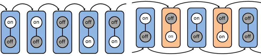
(a) Conventional CSMA algorithm (b) Proposed approach: Delayed CSMA
Figure 4.1: Comparison between the conventional CSMA and our proposed approach. A box indicates a schedule, and arrows indicate state transitions.
4.1
Delayed CSMA
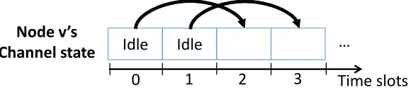
We start by giving an illustrative example showing why the CSMA algorithm tends to provide correlated link service process. Consider two links that are close to each other, so that only one link can be active at a time. At a particular moment, if a schedule of the two links is ‘active-inactive’, the inactive link first has to wait until the active link release the channel occupation. In this case, transition to next possible set of states is limited to ‘active-inactive’, and then ‘inactive-inactive states’. Direct transition to ‘inactive-active’ state is impossible. (See Figure 4.1a for example.) This phenomenon hinders a frequent switch between schedules, leading to starvation for the corresponding inactive link.
The method we propose in this paper effectively resolves this problem. The main idea is as follows. Suppose we have two schedulers that respectively generate schedules independently, while preserving the feasibility constraint for each time slot. If we choose to use one sched-uler at every odd time index, and the other one at every even time index (see Figure 4.1b), it is now possible to make a transition from ‘active-inactive’ directly to ‘inactive-active’ state, which would be impossible under the conventional CSMA. This alternate use of different sched-ulers produces more drastic change of states in consecutive time slots, thereby alleviating link starvation while maintaining the same long-term frequency of being active.
Algorithm 2 Delayed CSMA
1: Initialize: for all linksi∈ N,σi(t) = 0,t= 0,1, . . . , T−1.
2: At each time t≥T: links find a decision schedule, D(t) through a randomized procedure, and
3: for alllinks i∈ D(t) do
4: if P
j∈Niσj(t−T) = 0then
5: σi(t) = 1 with probability 1+λiλi
6: σi(t) = 0 with probability 1+1λi
7: else
8: σi(t) = 0
9: end if
10: end for
11: for alllinks j /∈ D(t) do
12: σi(t) =σi(t−T)
13: end for
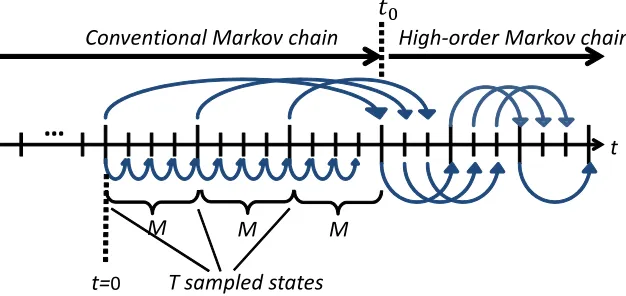
round-robin manner. Throughout the paper, we will use a notationT to indicate the number of such schedulers. In practice, this can be easily implemented in a distributed setting by having all links together update their schedules based on T-step-back state. For this purpose, each link only needs to remember its lastT channel states. This way, the whole system behaves as if there areT separate schedulers (or chains) taking turns to generate next schedules. Building upon this idea and applying to the CSMA scheduling, we next present our proposed algorithm, named delayed CSMA. Note that ifT = 1, our algorithm reduces to the conventional CSMA-based scheduling algorithm.
The key feature of our algorithm over the conventional one is that a new schedule is generated not from the current schedule but from T-step-back past schedule, and in doing so, each link just needs to make a decision based on its own T-step-back channel state information. Since every link operates this way, the independent set constraint is satisfied all the time. From an analytical point of view, however, this means that the evolution of schedule σ(t) is no longer a
Markov chain of orderT on the same state space Ω, as follows:
P{Xt=x|Xt−1=xt−1, . . . , X0=x0}
=P{Xt=x|Xt−1=xt−1, . . . , Xt−T=xt−T},
implying the current state depends uponT past history.1 Our algorithm can then be succinctly
written as
P{Xt=y |Xt−T =x}=P(x, y) (4.1)
where P(x, y), x, y ∈ Ω is the transition probability of the conventional Markov chain from state x to y.
We here collect several notations and simple facts that hold for finite state Markov chains [3, 53, 7] and will prove useful throughout the analysis. Consider a finite-state, ergodic Markov chainYn with its transition matrixP. For functions f, g: Ω→R, we define
hf,P(k)giµ ,
X
x,y∈Ω
f(x)g(y)µ(x)P(k)(x, y) =Eµ{f(Y0)g(Yk)},
whereµ is a probability distribution ofY0 on Ω, and P(k)(x, y) isk-step transition probability
of the chain Yn. For simplicity, we writehfiµ,hf,1iµ =Eµ{f(Y0)}. Also define
(P(k)f)(x),X
y∈Ω
P(k)(x, y)f(x) =E{f(Yk)|Y0=x}. (4.2)
For a (high-order) Markov chain Xt with order T as given in (4.1), if we define Ynm =XnT+m
for 0≤m≤T−1 andn= 0,1,2, . . ., then{Ym
n }n≥0 for eachmis a conventional Markov chain 1Alternatively, one can also augment the state space into a product space Ω× · · · ×Ω (T times) on which
{Xt−T+1, . . . , Xt−1, Xt}becomes a Markov chain. But, this would lead to largely intractable descriptions and keep
with initial state Ym
0 =Xm. Since the chain P is ergodic, we have, for any initial state x,
lim
k→∞(P
(k)f)(x) = lim k→∞
E{f(Ym
k )|Y0m=x}=hfiπ (4.3)
where π is the stationary distribution of the chain P. Since this holds for any given m = 0,1, . . . , T −1, it follows that
lim
t→∞
E{f(Xt)|X0 =x1, . . . XT−1=xT−1}=hfiπ,
implying that the marginal distribution ofXtin the steady-state remains the same and does not
change with T. However, we show next that different T leads to strikingly different behavior in the second order statistics.
Proposition 5. (Asymptotic zero-correlation padding) LetXt be a high-order Markov chain of
order T where the transition kernel is given by (4.1). For any initial distribution, if k 6= jT, j∈N,
lim
t→∞
E{f(Xt)g(Xt+k)}=hfiπhgiπ,
assuming that the expectations exist.
Proof. Writing t=nT +m, andt+k=n′T+m′ form, m′ ∈ {0, . . . , T−1}and n, n′= 0,1, . . ., one can verify that m 6=m′ if k6=jT. DefineYm
n =XnT+m, and Ym ′
n′ =Xn′T+m′. For given
m, m′, Ym
n and Ym ′
n′ are both conventional Markov chains with transition kernel P. Then by
conditioning, we have
E{f(Xt)g(Xt+k)}=E{f(Ynm)g(Ynm′′)}
=E{E{f(Ynm)g(Ym′
n′ )|Y0m, Ym ′
and observe that
E{f(Ym
n )g(Ym ′
n′ )|Y0m=i, Ym ′
0 =j}
=E{f(Ynm)|Y0m=i, Y0m′=j}E{g(Ym′
n′ )|Y0m=i, Ym ′
0 =j}
=E{f(Ym
n )|Y0m=i}E{g(Ym
′ n′ )|Ym
′
0 =j}
= (P(n)f)(i)(P(n′)g)(j)
where the first and second equalities follow from the conditional independence of Ym
n and Ym ′ n′
when initial values are fixed. Since n, n′ → ∞ as t → ∞, by taking limits and from (4.3), we are done.
Proposition 6. (Asymptotic correlation-lag shifting) Let Xt be a Markov chain of order T
with its transition kernel given by (4.1). For any initial distribution and for any given k∈N, we have
lim
t→∞E{f(Xt)g(Xt+kT)}=hf,P
(k)gi π,
assuming that the expectations exist.
Proof. As before, writet=nT+mform∈ {0,1, . . . , T−1}andn= 0,1, . . .. ThenYnm =XnT+m
for each m is a Markov chain. Observe that
E{f(Xt)g(Xt+kT)}=E{f(Ym
n )g(Ynm+k)}=hf,P(k)giµm n,
whereµmn is the distribution ofYnm. Since n→ ∞ ast→ ∞, taking limit gives
lim
n→∞hf,P
(k)gi µm
n =hf,P
(k)gi π,
sinceµmn ⇒π asn→ ∞ and the state space is finite. This completes the proof.
0 0.2 0.4 0.6 0.8 1
0 5 10 15 20 25 30
ψ
(k)
k
lag-shifting
zero-padding
T=1 T=5
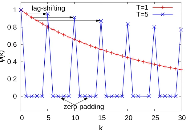
Figure 4.2: Two properties of the algorithm: correlation-lag shifting and zero-correlation padding
orderT (i.e., modeled asXt here), Propositions 5 and 6 tell us that the correlationsψ(k) under
our delayed CSMA algorithm with orderT are first shifted toT times larger lags, and then all padded with zero in-between. To see this effect numerically, we have run the simulations with the same step as in Figure 3.2, but now with T = 5. As seen in Figure 4.2, the correlations ψ(1), ψ(2), and ψ(3) for T = 1 case respectively gets shifted to ψ(5), ψ(10), and ψ(15) for T = 5, andψ(k) = 0 for allk6≡0 (mod 5). For the rest of the paper, we call these phenomena zero-padding and lag-shifting, respectively.
4.2
Delay Performance
now that the fugacity for each link is a fixed constant. This assumption will be relaxed later in Section 4.3, in which we show our algorithm under any finite T is also throughput optimal when the fugacity can be time-varying, set to be some function of the queue-length at each link. At this point, we focus on the long-term behavior of the delay, as any impact of transient phase will eventually fade away as time goes on, and in the standard queueing literature, the behavior of queue-length or delay is discussed mostly in the steady-state. We will briefly touch upon the impact of transient phase under our algorithm later in Section 4.4.
First, Little’s law asserts that the average delay is determined by the average queue length given that arrival rate is kept the same. For this reason, we are here interested in the stationary behavior of the queue-length driven by the recursion in (2.1). Let I(t) = A(t)−σ(t) be the net input to the queue at time t, with E{I(t)} = η−πB
v = −ξ < 0 for the stability of each queue [60]. LetAt=Ptk=1A(k) andSt=Ptk=1σ(k) be the cumulative amounts of arrival and
service overt slots, respectively. For a constantC such that C > ξ=πBv−η >0, we define
Z(t),A(t)−σ(t) +C, and Zt, t
X
k=1
Z(k). (4.4)
Then, it follows that the recursion in (2.1) can be written as
Q(t) = [Q(t−1) +Z(t)−C]+, (4.5)
i.e., the queue-length evolves as if the arrival process is Z(t) with E{Z(t)} = C−ξ and the service rate is constantC. Thus, the queue-length Q in the steady-state admits the following.
P{Q > x}=P
sup
t≥0
[Zt−Ct]> x
.
is arbitrary, this implies that T distinct sub-processes defined by σ(i)(n) = {σ(nT +i)} n≥0,
i= 1, . . . , T are all independent in the steady state, and the entire correlation structure of the original processσ(n) carries over to each of the sub-processσ(i)(n).
In particular, let Z(i)(n) = Z(nT +i), n ≥ 0, for each i = 1,2, . . . , T. From the zero-padding and lag-shifting properties, and since A(t) is i.i.d. over time t and also independent of σ(t), it follows that {Z(i)(n)}n≥0, i = 1,2, . . . , T are i.i.d. processes, each of which has
E{Z(i)(n)}=C−ξ and Cov{Z(i)(n), Z(i)(n+k)}= Cov{Z(n), Z(n+k)} in the steady state. If we consider a cumulative net-input process up to t = nT for some n ∈ N, then we can decomposeZt intoZt=PTi=1Z
(i) t where
Z(ti),
n−1
X
k=0
Z(i)(k) =A(ti)−S
(i) t +nC
=
n−1
X
k=0
[A(kT+i)−σ(kT +i) +C].
Thus, the cumulative ‘modified net-input’ process Zt to the queue with constant service rate of C is nothing but a superposition of T i.i.d. replicas of the original (Zt = PTi=1Z(
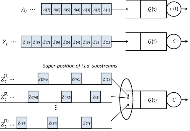
i) t ), but with its timescale stretched by T-fold. Our algorithm with parameter T thus effectively de-correlates the original service process (or the modified net-input process), regardless of how much correlations persist in the original case caused by any arbitrary topological constraint under the Glauber dynamics. See Figure 4.3 for illustration. Also,
P
sup
t≥0
[Zt−Ct]> x
=P
(
sup
t≥0 T
X
i=1
h
Z(ti)−(C/T)t
i
> x
)
.
In other words, the queue at linkv behaves as if we aggregateT i.i.d. input and also aggregate T different service capacities ofC/T each. Thus, we expect that the usual benefits of statistical multiplexing gain and the economies of scales [43, 6, 31], or the principle of “Sharing resources is always better than partitioning.” [46] should apply here.
(1) (2) (T) (T+1) (T+2) (2T)
…
…
…
…
(1) (2) (T) (t) (t)(2T+1)
(2T+2)
(3T)
(t)
…
(t)Super-position of i.i.d. substreams (4)
(5) (6)
(7) (3) (2) (1)
(4) (5) (6)
(7) (3) 2) (1) (8)
(8)
.
.
.
Figure 4.3: Our algorithm has an effect of dividing the original net-input process of a single stream (top) into a sum of i.i.d. substreams (bottom) in the steady state.
algorithm, we can also employ the usual Gaussian approximation for Zt, now a sum ofT i.i.d.
processes, by appealing to the Central Limit Theorem. Note that E{Zt} = (C −ξ)t and we define by v(t, T) the variance of Zt under our algorithm with order parameter T. Then, it
is known that the queue-length distribution with Gaussian input can be well approximated by [10, 18, 21]
P{Q > x} ≈exp
−inf
t>0
(ξt+x)2 2v(t, T)
(4.6)
for a wide range ofx >0. We then have the following.
Proposition 7. For any givent >0, v(t, T) is decreasing (non-increasing) in T >0.
Proof. Let σ(t, T) be the configuration state generated from our algorithm, a Markov chain
of order T, and set σ(t, T) = 1{σ(t, T) ∈ Bv} to be the service process of link v under our
algorithm with T. Since At is independent of the service process in any case, and doesn’t depend on T, it suffices to show that Var{Pt−1
k=0σ(k, T)} is non-increasing in T for any given
Define r(k, T) = Cov{σ(0, T), σ(k, T)} to be the covariance function in the steady state. We then have
Var
(t−1 X
k=0
σ(k, T)
)
=t·Var{σ(0, T)}+
t−1
X
k=1
(t−k)r(k, T).
Since the marginal distribution remains the same under our algorithm, Var{σ(0, T)} does not depend on T. Thus, it remains to show that the second term on the RHS is non-increasing in T. Notice that from Propositions 5 and 6, and by setting f(·) =g(·) =1{· ∈Bv}, we have
r(k, T) = 0, fork6=nT, n= 1,2, . . . (4.7) r(nT, T) =r(n,1),r(n), (4.8)
under our algorithm with parameter T. Now, observe that
t−1
X
k=1
(t−k)r(k, T)(4=.7)
t−1
X
k=T,2T,...
(t−k)r(k, T)
=
⌊(t−1)/T⌋
X
j=1
(t−jT)r(jT, T) (by letting k=jT)
(4.8)
=
⌊(t−1)/T⌋
X
j=1
(t−jT)r(j) ≥
⌊(t−1)/(T+1)⌋
X
j=1
(t−j(T+1))r(j)
(4.8)
=
⌊(t−1)/(T+1)⌋
X
j=1
(t−j(T+1))r(j(T+1),(T+1))
=
t−1
X
k=T+1,2(T+1),...
(t−k)r(k,(T+1))(4=.7)
t−1
X
k=1
(t−k)r(k,(T+1))
where the inequality holds since r(k) = ψ(k)Var{σ(k,1)} ≥ 0 from Proposition 3. This com-pletes the proof.
approach guarantees to reduce the variance of the cumulative net-input to the queue, which subsequently results in smaller queue-length.
4.3
Throughput Optimality
In this section, we consider how to adjust the parameter λv using queue information in order
to achieve throughput-optimality. In our algorithm, we set λv(t) = eWv(t) for some suitable
weight function of linkv. Although the link schedules under our algorithm are updated based on their T-step-back states, we set the weight function Wv(t) to be a function of the current
queue length Qv(t) at time t, rather than T steps ago, such that the system can react more
quickly by adjusting the dynamic fugacities with the latest information.
With the time-varying parameter, the state transition matrix becomes time-inhomogenous, which we write as Pt, a function of λv(t), v ∈ N at time t. For each given suchPt, we denote
by πt its unique stationary distribution (in a row vector form), i.e., πt =πtPt, and let µt be
the actual distribution of the link schedules σ(t) at time t under our algorithm with order
parameterT. In other words, we have
µt=µt−TPt−1. (4.9)
Similar to the steps via ‘network adiabatic’ theorem in [65, 68], a key step in proving the throughput optimality of our algorithm is to show that µt ≈ πt for sufficiently large queue
lengths under (4.9). The distance between two probability distributions is characterized by the notion of total variation (TV) distance [7, 53], defined as
kν−µkTV=
1 2
X
σ∈Ω
|ν(σ)−µ(σ)|.
slowly over time t for all large queue-lengths. (In fact, this can be achieved by setting the weight function Wv(t) as a very slowly increasing function of the queue-length [65, 23, 68].)
Then, the resulting πt, a solution to π = πPt is also slowly varying over time t such that the
actual distribution µt is able to get closer to πt (in the sense of TV distance) before πt moves
away to another, thus effectively simulating the separation of timescales. As will be shown in Section 4.4, under our algorithm with order parameterT, the speed of convergence ofµtunder
static fugacity (i.e., static P) is roughly T times slower than that of the conventional Glauber dynamics. This implies that the speed of actual distribution µt under dynamic fugacity as a
slowly varying function of queue-length, will also be reduced by a factor ofT. SinceT is finite, we expect thatµtis still able to catch up the slowly varying targetπtin time, and by following
similar steps in [65, 23, 68] our algorithm can also achieve the throughput optimality. Our next result below shows that this is indeed the case.
Proposition 8. Let ǫ > 0 be arbitrarily given. For any arrival rate η ∈ (1−ǫ)C, set the
dynamic link weight2
Wv(t) = max
h(Qv(t)), ǫ
2|N |h(Qmax(t))
, (4.10)
where h(·) = log log(·+e). Then, our algorithm with any finite order parameter T satisfies (2.2), and is thus throughput optimal.
Proof. See Appendix.
Proposition 8 together with our delay analysis in Section 4.2 assert that our algorithm with order T achieves not only the required throughput optimality, but also much better delay performance by effectively cutting down the dependency among consecutive link states, thus promoting much faster link state changes, while keeping all the marginal distributions the same.
2Q
max(t) is the length of the largest queue in the network at time t. In [65] it is argued thatQmax(t) can
be easily estimated via any gossip-like message passing mechanism. The use ofQmax(t) is for purely technical
reasons, and it doesn’t need to be known in practice, as conjectured in [65, 68]. For simplicity, we assumeQmax(t)