ABSTRACT
FENG, JINYONG. Evaluation of Interfacial Forces and Bubble-Induced Turbulence Using Direct Numerical Simulation (Under the direction of Dr. Igor A. Bolotnov).
High fidelity prediction of multiphase flows is important in a wide range of engineering
applications. While some multiphase flow scenarios can be successfully modeled, many questions remain unanswered regarding the interaction between the bubbles and the
turbulence, and present significant challenges in the development of closure laws for the multiphase computational fluid dynamics (M-CFD) models. To address these challenges, we propose to evaluate the interfacial forces and bubble-induced turbulence in both laminar and
turbulent flow field with direct numerical simulation (DNS) approach.
Advanced finite-element based flow solver (PHASTA) with level-set interface tracking
method is utilized for these studies. The proportional-integral-derivative (PID) controller is adopted to ensure the statistically steady state bubble position and perform the detailed study of the turbulent field around the bubble. Selected numerical capabilities and post-processing
codes are developed to achieve the research goals. The interface tracking approach is verified and validated by comparing the interfacial forces with the experiment-based data and
correlations. The sign change of transverse lift force is observed as the bubble becomes more deformable. A new correlation is proposed to predict the behavior of the drag coefficient over the wide range of conditions. The wall effect on the interfacial forces are also investigated. In
homogeneous turbulent flow, the effect of bubble deformability, turbulent intensity and relative velocity on the bubble-induced turbulence are analyzed. The presented method and
Evaluation of Interfacial Forces and Bubble-Induced Turbulence Using Direct Numerical Simulation
by Jinyong Feng
A dissertation submitted to the Graduate Faculty of North Carolina State University
in partial fulfillment of the requirements for the degree of
Doctor of Philosophy
Nuclear Engineering
Raleigh, North Carolina
2017
APPROVED BY:
_______________________________ _______________________________ Prof. Igor A. Bolotnov Prof. Nam Dinh
DEDICATION
BIOGRAPHY
The author, Jinyong Feng, was born on September 30th, 1989, a year of snake in Chinese calendar. The family name, Feng, originates from a war hero during the Spring and Autumn period (from approximately 771 to 476 BC) in Chinese history. The first word of the
given name, Jin, is shared by all his cousins and has the meaning of gold. The second word of the given name, yong, is given by his father and it means the bravery. His father wishes him to be fearless and explore the outside world.
As the second child in the family, he received high expectation from his parents, especially when he had an outstanding elder sister. His sister was academically always the #1
in their primary and middle school and then went to the #1 university in China, Peking University. The existence of his sister encouraged him to keep challenging himself and breaking through the limits. His mottos of the life is “one’s life must matter”.
He went to one of the top universities (but not #1) in China, University of Science and Technology of China (USTC), and graduated with the Bachelor’s degree in Nuclear
Engineering. About 40% of the graduates in USTC will go to U.S. to pursue advanced degrees, like Master’s degree and Ph.D. So the USTC gained a nickname of “United Stated Training Center” in China. Among one of those students, Jinyong was also looking forward to the
outside world and making differences in his life. Soon after his graduation, he came to the Texas A&M University. The life in Texas is very enjoyable and the author got a Master’s
Traveling and sports are his favorite hobbies. Traveling is a great way to explore the beauty of the world and enrich the knowledge. He has visited 29 states of America and gained
many great memories, the magnificent Grand Canyon, the bizarre skyline of New York City, -20 oC chilly temperature of Minnesota, the fabulous Las Vegas, etc. As a crazy basketball fan, one of his lifetime goal is to visit all the home stadiums of the NBA teams. He has visited 24 stadiums and only 5 are left now, Boston Celtics, Portland Trail Blazers, Sacramento Kings, Toronto Raptors and Utah Jazz. The Ph.D. is a milestone in his life, but there are numerous
ACKNOWLEDGMENTS
I am incredibly thankful to my family. My parents worked very hard to ensure that I
can receive the best education. Their great personalities and diligence served as the role model of my entire life. My elder sister gives me lots of helpful advices on my entire career and
inspires me to keep pushing myself to the next level. My nephew is almost 3 years now and he is so adorable. My family is the most valuable treasure of my life and I wish to become the one they can be proud of.
I would like to express my sincerest thanks to Dr. Igor A. Bolotnov for all his guidance and help. Dr. Bolotnov brought me into the beautiful world of two-phase bubbly flow and
taught me the solid theoretical knowledge, self-motivated research attitude, critical thinking capability and technical writing skills. He helped me grow from a fresh graduate to a serious researcher.
I also want to give thanks to my research group members. Dr. Jun Fang was my undergraduate classmate and we have known each other for almost 8 years. His brilliant
guidance and friendly help made me quickly familiarize myself with our research code— PHASTA. We had lots of collaborations on various research topics and it was really enjoyable to work with him. Mr. Aaron Thomas built the foundation of the PID bubble controller and it
had incredible value for my research and accelerated my research progress. Dr. Cameron Brown helped me a lot on my thesis and gave me some innovative ideas. The discussion of
turbulence theory with him is very beneficial for my research.
are world-renowned professors. Their brilliant guidance and thoughtful suggestions helped me improve my understanding on the two-phase bubbly flow phenomena. Many of the faculty,
staff, and graduate students in the Department of Nuclear Engineering at NCSU gave me valuable help and assistance. In particular: Dr. J. Michael Doster, Dr. Jack Edwards, Dr. Maria
Avramova, Dr. Hong Luo, Dr. Jason Hou, Dr. Koruhonda Murty, Ms. Hermine Kabbendjian, Ms. Lisa Marshall, Mr. Mario Milev, Mr. Yuwei Zhu, Mr. Guojing Hou, Mr. Han Bao, Mr. Chih-Wei Chang, Mr. Hao-Ping Chang, Ms. Mengnan Li, Mr. Yangmo Zhu, Mr. Kaiyue Zeng,
Ms. Ting-yi Wang, Ms. Paulina Duckic, etc. I also wanted to express my appreciation to Dr. William D. Pointer for his guidance at Oak Ridge National Lab (ORNL). During the 10-weeks
internship, he helped me gain practical experience on developing two-phase boiling model using industrial standard software. His enthusiastic work spirit is very impressive.
Finally, I would like to acknowledge the support from the National Science
Foundation—United States (award 13339933 under CBET-Fluid Dynamics Program). Some of the computational resources were supported by U.S. Nuclear Regulatory Commission’s
Faculty Development Program. An award of computer time was provided by the ASCR Leadership Computing Challenge (ALCC) program. This research used resources of the Argonne Leadership Computing Facility, which is a DOE office of Science User Facility
supported under Contract DE-AC02-06CH11357. The solution presented herein made use of the Acusim linear algebra solution library provided by Altair Engineering Inc. and mesh and
TABLE OF CONTENTS
LIST OF TABLES ... xi
LIST OF FIGURES ... xiii
LIST OF SYMBOLS OR ABBREVIATIONS ... xxiii
CHAPTER 1. INTRODUCTION ... 1
1.1 Overview and motivation ... 1
1.2 Turbulence modeling and simulation ... 6
1.3 Decay of homogeneous turbulence ... 9
1.4 Multiphase flow modeling ... 11
1.5 Interfacial forces in M-CFD ... 18
1.5.1 Drag force ... 19
1.5.2 Lift force ... 22
1.5.3 Virtual mass force ... 25
1.5.4 Wall force ... 26
1.5.5 Turbulent dispersion force ... 29
1.6 Wall effect on interfacial forces and BIT ... 29
1.7 Bubble-induced turbulence theory ... 34
1.7.1 Experimental work ... 35
1.7.2 Numerical simulations ... 40
1.8 Influence of the BIT on the interfacial forces ... 42
2.1 PHASTA overview ... 46
2.1.1 Governing equations ... 48
2.1.2 Level-set method ... 49
2.2 PID bubble controller ... 53
2.3 Turbulence generation algorithm ... 59
2.3.1 Homogeneous uniform turbulent flow generation ... 59
2.3.2 Shear turbulent flow generation ... 65
2.4 Parallel BCT file computing capability ... 69
2.5 Data analysis algorithm ... 74
CHAPTER 3. INTERFACIAL FORCES EVALUATION ... 77
3.1 Evaluation of lift force under laminar shear flow ... 77
3.1.1 Mesh independence study ... 79
3.1.2 Results and discussion ... 84
3.2 Evaluation of wall effect under laminar shear flow ... 90
3.2.1 The effect of wall distance ... 91
3.2.2 The effect of relative velocity ... 95
3.2.3 The effect of bubble deformation ... 97
3.3 Evaluation of drag force under homogeneous turbulent flow ... 101
3.3.1 The effect of turbulent intensity ... 108
3.3.2 The effect of bubble deformability ... 112
3.3.3 The effect of relative velocity ... 114
4.1 Evaluation of BIT in homogeneous turbulent flow ... 117
4.1.1 Validation of level-set approach for BIT problem ... 119
4.1.2 The effect of turbulent intensity ... 126
4.1.3 The effect of bubble deformability ... 129
4.1.4 The effect of relative velocity ... 136
CHAPTER 5. SHEAR TURBULENT FLOW ... 138
5.1 Low shear turbulent flow ... 138
5.2 High shear turbulent flow ... 142
CHAPTER 6. CONCLUSIONS ... 147
CHAPTER 7. FUTURE WORK RECOMMENDATIONS ... 149
7.1 In-line motion of two bubbles and wake interaction ... 149
7.2 Interfacial forces of single bubble in turbulent boundary layers ... 152
7.3 Data-driven analysis on the wall effect study ... 154
7.4 BIT in shear turbulent flow field ... 157
7.5 Verification of incompressibility assumption ... 158
7.6 Closure law development—virtual mass and turbulent dispersion forces ... 159
REFERENCES ... 163
APPENDICES ... 178
Appendix A ... 179
Appendix B ... 180
LIST OF TABLES
Table 1. Constants used in the 𝒌𝒌 − 𝜺𝜺 model. ... 15
Table 2. Drag coefficients at different bubble Reynolds numbers. ... 57
Table 3. Geometrical and mesh configuration of the single phase homogeneous turbulent flow case. ... 63
Table 4. Summary of the mesh study results. ... 82
Table 5. Case setup of lift force evaluation study. ... 85
Table 6. Statistics of the simulation and experiment results for the lift force evaluation study. ... 86
Table 7. Comparison of the simulation and experiment results for lift force evaluation study. ... 88
Table 8. Summary of the wall distance cases setup. ... 91
Table 9. Summary of the bubble Reynolds number cases setup. ... 95
Table 10. Summary of the bubble deformation cases setup. ... 98
Table 11. Fluid properties summary for drag force evaluation case... 104
Table 12. Summary of the bubble deformability study. ... 113
Table 13. Summary of the relative velocity study. ... 115
Table 14. Geometrical and mesh configuration of the level-set validation cases. ... 121
Table 15. Summary of the low shear single phase turbulent flow cases. ... 141
Table 16. Summary of the high shear single phase turbulent flow cases. ... 143
LIST OF FIGURES
Figure 1. A sketch of a turbulence-generating grid composed of bars of diameter d, with
mesh spacing M [27]. ... 11 Figure 2. Illustration of the migration direction for spherical and deformable bubble. 𝑢𝑢𝑢𝑢𝑢𝑢𝑢𝑢𝑢𝑢𝑢𝑢𝑢𝑢𝑢𝑢 represents the lateral migration velocity of the bubble, 𝑢𝑢𝑢𝑢 and 𝑢𝑢𝑢𝑢 represent the
streamwise velocity of the bubble and liquid, respectively. ... 25 Figure 3. Comparison of bubble and liquid velocity distributions in Serizawa’s experiment [123]. ... 36
Figure 4. Comparison of the bubble volume evolution of a selected case for turbulent intensity study. Solid and dash lines represent the instantaneous void fraction and the expected
void fraction, respectively. ... 51
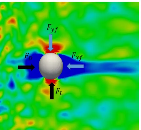
Figure 5. Illustration of the force balance acting on the bubbles. 𝐹𝐹𝐹𝐹, 𝐹𝐹𝐹𝐹, 𝐹𝐹𝐹𝐹𝐹𝐹 and 𝐹𝐹𝐹𝐹𝐹𝐹 represent the drag force, lift force, streamwise (x) direction control force and lateral (y)
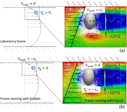
direction control force, respectively. ... 53 Figure 6. Transformation of inertial frame for wall effect on interfacial forces study. .... 55
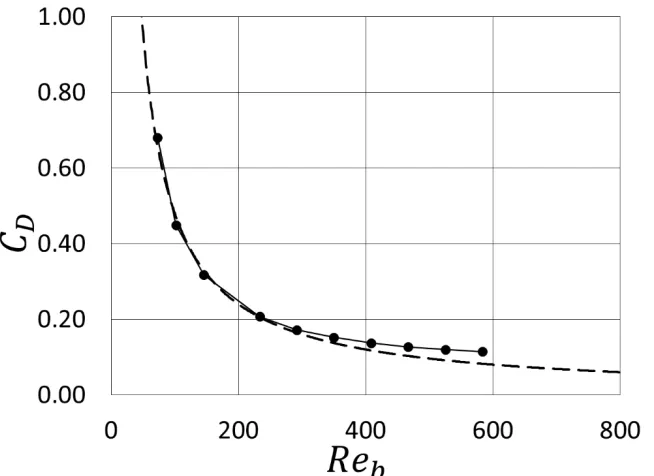
Figure 7. Estimated drag coefficient from PHASTA simulation (solid line with symbols) as a function of bubble Reynolds number. Dashed line shows Tomiyama’s experiment-based correlation [1]... 58
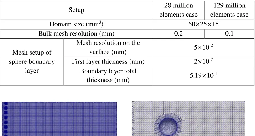
Figure 10. Geometric configuration of a single cell on the obstacle grid planes... 61 Figure 11. Mesh configuration of the homogeneous turbulence generation case. (a) shows
the mesh configuration of the whole domain; (b) shows the mesh configuration and boundary layer on the obstacle sphere surface... 63
Figure 12. 3D view of the homogeneous turbulent flow generation. ... 65 Figure 13. Measurement of turbulence statistics for three consecutive windows and each has a time window of 1.86 s. Dot, dash, dash-dot and solid lines represent the time window 1,
the time window 2, the time window 3 and the entire time window containing all three windows, respectively. ... 65
Figure 14. Illustration of turbulent flow generation using non-uniform grid distribution [169]. ... 66
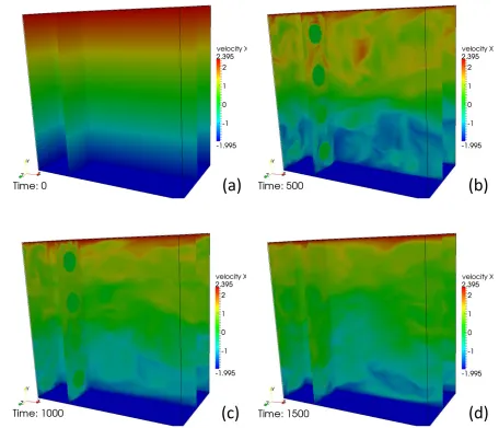
Figure 15. Shear turbulent flow generation at various simulation time steps. ... 68
Figure 16. Flowchart of BCT files’ generations and implementations. ... 69 Figure 17. Partition of the simulation domain to 64 cores where vtkCompositeIndex
represents the ID of the cores. (a) shows the partition where all the nodes on the inflow surface are assigned to the master core; (b) shows the new partition using the new parallel computing approach. ... 71
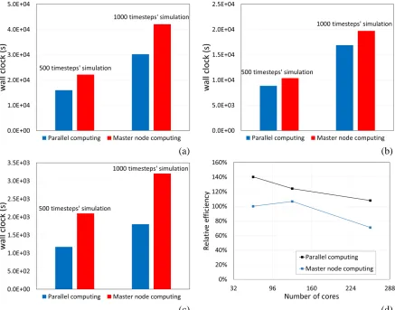
Figure 18. Evaluation of the computational performance of the new parallel BCT files computing capability. (a) to (c) are the computational performance for the cases running on
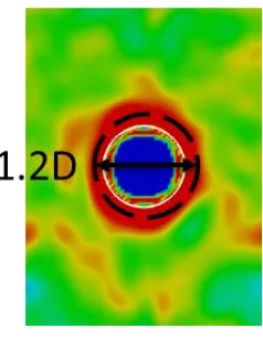
Figure 19. Diagram of averaging algorithm for two-phase simulation. White circle represents the bubble-liquid interface and the probes inside the dashed circle are excluded for
the data averaging. ... 76 Figure 20. Sensitivity analysis (bubble-induced turbulence versus streamwise position) of
screening windows for two different bubble deformation levels, We=1.35 (a) and 2.03 (b). The diameter of the exclusion circles are 1.1, 1.2, 1.5, and 2.0D. ... 76
Figure 21. Mesh configuration of the mesh study cases. The images from (a) to (d)
represent the case with 25, 35, 45 and 55 elements across bubble diameter. Both (e) and (f) represent the case with 65 elements across equivalent spherical bubble diameter. ... 80
Figure 22. Comparison of control force in streamwise (x) direction for mesh study. Mesh type 1 to 5 represent the 25, 35, 45, 55 and 65 elements across bubble diameter, respectively. ... 81
Figure 23. Comparison of lateral control force in lateral (y) direction for mesh study. Mesh type 1 to 5 represent the 25, 35, 45, 55 and 65 elements across bubble diameter, respectively.
... 81 Figure 24. GCI of drag coefficient versus various mesh setups. ... 84 Figure 25. Mesh configuration of the Parasolid model case with D=2.84 mm. ... 85
Figure 26. Evolution of control force in streamwise (x) direction for the lift force evaluation study. ... 87
Figure 28. Lift coefficient versus Eotvos number. (a) shows the 𝐶𝐶𝐹𝐹 versus 𝐸𝐸𝐸𝐸𝐸𝐸 for
different experiment data and DNS simulation; (b) shows the 𝐶𝐶𝐹𝐹 versus 𝐸𝐸𝐸𝐸 from DNS simulation. ... 90
Figure 29. Evolution of the control forces versus different wall distances, 𝐹𝐹/𝐹𝐹. ... 92 Figure 30. Drag and net lift coefficients (Eq.( 46 )) versus different wall distances. (a)
shows the drag coefficient versus 𝐹𝐹𝐹𝐹. (b) compares the lift coefficient based on the PHASTA data, Hosokawa’s correlation, and Tomiyama’s correlation. ... 92
Figure 31. Comparison of the pressure field for different wall distances (𝐹𝐹𝐹𝐹 = 0.625, 1.0 and 1.25) where the white line represents the pressure equal to -5 Pa. ... 93
Figure 32. Comparison of the streamline pattern for different wall distances (𝐹𝐹𝐹𝐹 = 0.625, 1.0 and 1.25). ... 93
Figure 33. Mesh refinement study. (a) shows the baseline mesh used in the wall distance study. (b) shows the case with extended mesh refinement region. ... 94
Figure 34. Comparison of the pressure fields for baseline mesh and extended mesh configurations. ... 94
Figure 35. Comparison of the control forces for baseline mesh (black line) and extended
mesh (red line) configurations. ... 95 Figure 36. Evolution of control forces versus bubble Reynolds number. ... 96
Figure 38. Comparison of velocity field for different bubble Reynolds numbers. The range
of legend for each figure is based on the velocity profile, 𝑉𝑉 = 3.8 ×𝐹𝐹+𝑢𝑢𝑢𝑢 and the values of 𝑢𝑢𝑢𝑢 are different for each case. ... 97
Figure 39. Evolution of the control forces versus bubble deformation levels. ... 99
Figure 40. Drag and net lift coefficients versus 𝐸𝐸𝐸𝐸. (a) shows the drag coefficient versus 𝐸𝐸𝐸𝐸. (b) compares the lift coefficients with the case where the bubble is far away from the wall, 𝐹𝐹𝐹𝐹 = 2.55. ... 99
Figure 41. Comparison of pressure fields for different bubble deformation levels. Three pressure contours of 5, 0, and -5 Pa are shown. ... 100
Figure 42. Comparison of streamline patterns for different bubble deformation levels. 100
Figure 43. Lift coefficient map 𝐶𝐶𝐹𝐹(𝑅𝑅𝑢𝑢𝑅𝑅,𝑊𝑊𝑢𝑢) at 𝐹𝐹𝐹𝐹 = 1. Red and blue symbols represent negative and positive lift coefficient, respectively. The data sources are from Sugioka and
Sugioka and Tsukada’s DNS data (sphere) [101], Takemura et al.’s experimental data (square) [102], and PHASTA’s DNS data (triangle). ... 101
Figure 44. Left image shows the generation of homogeneous turbulent flow. The dashed
rectangle indicates the probe plane. The simulation on the right utilizes the inflow recorded on the left. ... 102
Figure 45. Velocity (dash-dot line) and turbulent kinetic energy (solid line) profiles versus spanwise direction (y) for the single-phase homogeneous turbulent flow. ... 103
Figure 46. Simulation domain of drag force evaluation case. (a) and (b) show the velocity
Figure 47. Comparison of the bubble position evolution in streamwise (x) direction with lateral control force (black line) and without lateral control force (red line) for the validation
of PID bubble controller. ... 106 Figure 48. Comparison of the bubble position evolution in y direction with lateral control
force (black line) and without lateral control force (red line) for the validation of PID bubble controller. ... 107
Figure 49. Comparison of the bubble position evolution in z direction with lateral control
force (black line) and without lateral control force (red line) for the validation of PID bubble controller. ... 107
Figure 50. Comparison of the streamwise (x) direction control force with lateral control force (solid line) and without lateral control force (dash line) for the verification of PID bubble controller. The control forces are averaged over separate windows (square symbols) and over
the whole time range (no symbols), respectively... 108 Figure 51. Different bubble positions for the turbulent intensity effect study. Bubble local
turbulent intensities from left to right are, 3.44%, 2.86% and 2.34%, respectively. ... 110 Figure 52. Evolution of streamwise direction (x) control force for the turbulent intensity effect study. ... 111
Figure 53. Comparison of the drag coefficient from PHASTA simulation (square symbols), the drag coefficient from Tomiyama’s correlation (dash-dot line) and the control force
Figure 55. Comparison of the drag force (solid line), the drag coefficient for homogeneous turbulent flow condition (dash line) and the drag coefficient for laminar flow condition
(dash-dot line) versus different bubble deformation levels. ... 114 Figure 56. Comparison of bubble shape for different relative velocities. ... 115
Figure 57. Drag coefficient comparison between Tomiyama’s correlation and DNS-based correlation. Data point from laminar flow simulation has been reported in [56]. ... 116
Figure 58. Velocity and turbulent kinetic energy profiles for different mesh refinement.
Solid and dotted lines represent 28 million and 129 million mesh cases, respectively. ... 118
Figure 59. Decay of turbulent kinetic energy as a function of 𝐹𝐹𝑥𝑥. Solid and dash lines represent raw data and power approximation line, respectively. ... 119
Figure 60. Simulation domain for level-set verification cases. ... 121 Figure 61. Density evolution across the interface. The width of the transition region are 1 (hollow sphere), 2 (hollow square), 3 (triangle), 4 (square) and 5 (sphere) elements. ... 122
Figure 62. TKE profile from probe plane 1 versus different artificial interface thicknesses, 0 (no interface), 0.025 D, 0.05 D, 0.25 D and 0.5 D where D is the sphere diameter. Left (a)
and right (b) represent the plot at probe plane 1 and 2 (described in Table 14), respectively. ... 123 Figure 63. Velocity profile versus different artificial interface thicknesses for probe plane
1... 123 Figure 64. Relative error versus artificial interface thickness for two locations in the wake
Figure 65. Comparison of pressure field for different interface thicknesses, 𝜀𝜀𝐹𝐹=0.96, 0.16, and 0.24. ... 125
Figure 66. Turbulent intensity versus position for different interface thicknesses cases, 𝜀𝜀𝐹𝐹=0.96 (square), 0.16 (triangle), and 0.24 (sphere), where 𝐹𝐹/𝐹𝐹=0 represents the streamwise
position of the bubble center. ... 126
Figure 67. Turbulent intensity versus position for different bubble local turbulent intensity cases, 3.44% (square), 2.86% (circle) and 2.34% (triangle). The center of the bubble
corresponds to the 𝐹𝐹𝐹𝐹 = 0. ... 127 Figure 68. Turbulent isotropy comparison for different turbulent intensities. Bubble
positions are 2.00, 3.14 and 4.93 for different turbulent intensities cases. ... 129 Figure 69. Turbulent intensity versus non-dimensional position with different bubble
deformation levels. The center of the bubble corresponds to the 𝐹𝐹𝐹𝐹 = 0. ... 130 Figure 70. Bubble shape evolution over time. Bubble shape remains stable until time t = 0.82 s and becomes unstable after that. ... 133
Figure 71. Comparison of streamline pattern around spherical and deformable bubble. 134 Figure 72. Turbulent eddies generation on the highly deformable bubble surface. The
contour is plotted using Q-criterion with value of 100. ... 135 Figure 73. Comparison of turbulent intensity versus position with different bubble deformation levels. For the highly deformable bubble, We=3.39, the stable period, shape
Figure 74. Turbulent intensity versus position with different relative velocity. Solid and dash lines represent the two-phase and single-phase cases, respectively. ... 137
Figure 75. Illustration of the boundary conditions for the generation of shear turbulent flow. ... 139
Figure 76. Evolution of velocity field for shear turbulent flow cases with initial shear rate of 30 s-1. (a) and (b) shows the velocity field when a 2×4 array of obstacle spheres are present. ... 140 Figure 77. Comparison of TKE and velocity profiles for different initial shear rates, 30
(dash-dot line), 45 (dash line), and 60 (solid line). ... 141 Figure 78. Comparison of turbulent isotropies for different initial shear rates, 45 (left
figure), and 60 (right figure) s-1. ... 141 Figure 79. Refinement boundary layers near the wall for high shear turbulent flow simulations. ... 143
Figure 80. Law of the wall profile for high shear turbulent flow simulations. ... 144 Figure 81. Comparison of turbulent eddies for different high shear turbulent flow cases. (a)
to (c) represent the near wall shear rate, 𝑑𝑑𝑢𝑢𝑑𝑑𝐹𝐹𝑑𝑑𝑢𝑢𝑢𝑢𝑢𝑢, from 768.2 to 1307.0 s-1. The contours are plotted by Q-criterion with value of +25000. ... 145
Figure 82. Comparison of TKE and velocity profiles for different near wall shear rates, 768.2 (solid line), 1071.2 (dash-dot line) and 1307.0 (dot line) s-1. ... 145
Figure 85. Evolution of the interaction between the bubble and wake region of hemisphere. ... 151
Figure 86. Evolution of streamwise control force for the study of the interaction between leading hemisphere and trailing bubble. ... 152
Figure 87. Full 3D replica of boundary conditions using BCT capability... 153 Figure 88. Wall normal velocity profile of high shear turbulent flow. ... 154 Figure 89. Illustration of neural network layout for wall effect study. ... 156
Figure 90. Mesh configuration of the wall effect study where the dash-dot rectangle represents the reserved region for future neural network study. ... 156
Figure 91. Single bubble immersed in high shear turbulent flow field where the initial shear rate is 1250 s-1. The contour is plotted by Q-criterion and has constant value as +6×10⁶ m/s2 ... 158 Figure 92. Trajectory of single bubble with constant acceleration in streamwise position.
... 160 Figure 93. Single bubble in low shear turbulent flow field. (a) shows the shear velocity
field around the bubble and (b) shows the single-phase streamwise velocity profile versus wall-normal position (y). ... 161 Figure 94. Illustration of bubble-bubble interaction in shear turbulent flow field. (a) and
LIST OF SYMBOLS OR ABBREVIATIONS Abbreviation
3D Three dimensional
BIT Bubble-induced turbulence BCT Boundary condition transient data CFD Computation fluid dynamics DES Detached eddy simulation DNS Direct numerical simulation
E-E Eulerian-Eulerian approach E-L Eulerian-Lagrangian approach FEM Finite element method
GCI Grid convergence index
HOT Higher order terms of truncation error HPC High performance computing
ITM Interface tracking method LES Large eddy simulation
M-CFD Multiphase computational fluid dynamics PDE Partial differential equation
PHASTA Parallel, Hierarchic, Adaptive, Stabilized, Transient Analysis flow solver RANS Reynolds-Averaged Navier-Stokes equations
TKE Turbulent kinetic energy VOF Volume of fluid
Notation
𝐴𝐴 Bubble cross-sectional area (m2) 𝐴𝐴′′′ Interfacial area density (m-1)
𝐵𝐵 Constant used in “log law”
𝐶𝐶 Coefficient for power decay law of turbulent kinetic energy
𝐶𝐶𝐵𝐵 Coefficient of bubble-induced turbulence eddy viscosity for Sato’s model
𝐶𝐶𝐷𝐷 Drag coefficient
𝐶𝐶𝜀𝜀1 Constants used in 𝑘𝑘 − 𝜀𝜀 model
𝐶𝐶𝐿𝐿𝐷𝐷 Modified lift coefficient
𝐶𝐶𝜇𝜇 Constants used in 𝑘𝑘 − 𝜀𝜀 model
𝐶𝐶𝑇𝑇𝐷𝐷 Turbulent dispersion coefficient
𝐶𝐶𝑝𝑝 Potential flow solution coefficient
𝐶𝐶𝑇𝑇 Net transverse lift coefficient
𝐶𝐶𝑉𝑉𝑉𝑉 Virtual mass coefficient
𝐶𝐶𝑊𝑊 Wall coefficient
𝐶𝐶𝐹𝐹𝑖𝑖(𝑛𝑛) 𝑖𝑖𝑡𝑡ℎ component of the control force at time 𝑛𝑛 𝑑𝑑 Scalar in re-distancing equation (m)
𝐹𝐹 Spherical bubble diameter (m) 𝐹𝐹𝐻𝐻 Extended bubble diameter (m)
𝐹𝐹
𝐹𝐹𝑢𝑢 Substantial derivatives
𝐸𝐸𝑜𝑜 Spherical bubble-based Eotvos number
𝐸𝐸𝑜𝑜𝐻𝐻 Extended bubble-based Eotvos number 𝐹𝐹 Body force term
𝐹𝐹𝐷𝐷 Drag force (N)
𝐹𝐹𝐿𝐿 Lift force (N)
𝐹𝐹𝑠𝑠 Factor of safety in GCI
𝐹𝐹𝑇𝑇𝐷𝐷 Turbulent dispersion force (N)
𝐹𝐹𝑉𝑉𝑉𝑉 Virtual mass force (N)
𝐹𝐹𝑊𝑊 Wall force (N)
𝐸𝐸𝜀𝜀 Heaviside kernel function
𝐼𝐼 Turbulent intensity
𝑘𝑘 Liquid turbulent kinetic energy (m2/s2)
𝐹𝐹 Distance between bubble center and the wall (m) 𝑥𝑥 Spacing between two grids (m)
𝑥𝑥𝑘𝑘 Momentum exchange term of phase k (kg/(m2.s2))
𝑥𝑥𝑘𝑘𝐷𝐷 Momentum exchange term of phase k caused by drag force (kg/(m2.s2))
𝑥𝑥𝑘𝑘𝐿𝐿 Momentum exchange term of phase k caused by lift force (kg/(m2.s2))
𝑥𝑥𝑘𝑘𝑉𝑉𝑉𝑉 Momentum exchange term of phase k caused by virtual mass force (kg/(m2.s2)) 𝑥𝑥𝑘𝑘𝑇𝑇𝐷𝐷 Momentum exchange term of phase k caused by turbulent dispersion force (kg/(m2.s2))
𝑥𝑥𝐸𝐸 Morton number 𝑛𝑛 Power decay exponent 𝑛𝑛𝑤𝑤 Unit normal vector
𝑁𝑁𝑝𝑝 Number of phases in M-CFD governing equations
𝑝𝑝 Pressure (N/m2) 𝑄𝑄 q-criterion (s-2) 𝑅𝑅𝑢𝑢 Reynolds number
𝑅𝑅𝑢𝑢𝑏𝑏 Bubble Reynolds number
𝑅𝑅𝑢𝑢𝜏𝜏 Friction Reynolds number
𝑆𝑆 Strain rate tensor (m/s) 𝑆𝑆𝑢𝑢 Non-dimensional shear rate
𝑢𝑢 Time (s)
𝑑𝑑��⃗ Pseudo velocity in re-distancing equation (m/s) 𝑊𝑊𝑢𝑢 Weber number
𝑢𝑢 Streamwise direction (x) velocity (m/s) 𝑢𝑢� Mean velocity (m/s)
𝑢𝑢′ Root-mean-square of the turbulent velocity fluctuations (m/s) or instantaneous velocity fluctuation (m/s) 𝑢𝑢𝐸𝐸′ 2 Excess turbulent kinetic energy (m2/s2)
𝑢𝑢𝑔𝑔 Gas velocity (m/s)
𝑢𝑢𝑙𝑙 Liquid velocity (m/s)
𝑢𝑢𝑟𝑟 Relative velocity between liquid and gas (m/s)
𝑢𝑢𝜂𝜂 Kolmogorov velocity scale (m/s)
𝑢𝑢′𝑢𝑢′
������, 𝑣𝑣′𝑣𝑣′�����, 𝑑𝑑′𝑑𝑑′
������ Reynolds stress terms (m2/s2)
𝑈𝑈𝑜𝑜 Mean streamwise velocity in wind tunnel experiment (m/s)
𝑈𝑈 Mean velocity (m/s)
𝑣𝑣 Wall normal (y) direction velocity (m/s) 𝑉𝑉𝑏𝑏 Bubble volume (m3)
𝑑𝑑 Lateral (z) direction velocity (m/s) 𝐹𝐹 Streamwise (x) direction coordinate (m) 𝐹𝐹𝑜𝑜 Virtual origin in wind tunnel experiment (m)
Greek letters
𝛼𝛼 Void fraction
𝛼𝛼𝑔𝑔𝑠𝑠 Void fraction in the small bubble region
𝛿𝛿 Channel width (m)
𝜀𝜀 Turbulence dissipation rate (m2/s3)
𝜀𝜀𝑙𝑙 Interface half-thickness in level-set equation (m)
𝜀𝜀𝑑𝑑 Interface half-thickness in re-distancing equation (m)
𝜂𝜂 Kolmogorov length scale (m)
𝜂𝜂𝑗𝑗𝑖𝑖 Computing efficiency, where approach and 𝑗𝑗 represents the number of partitions 𝑖𝑖 represents the bct file computing
𝜅𝜅 Constants used in constant used in “log law” 𝑘𝑘 − 𝜀𝜀 model or curvature of gas-liquid interface or the 𝜆𝜆 Taylor length scale (m)
𝜑𝜑 Scalar in advection equation (m) 𝜙𝜙𝑠𝑠𝑟𝑟 Dimensionless drag multiplier
𝜎𝜎𝑘𝑘 Constants used in 𝑘𝑘 − 𝜀𝜀 model
𝜇𝜇𝐵𝐵𝐵𝐵𝑇𝑇 Bubble-induced turbulence dynamics viscosity (N.s/m2)
𝜇𝜇𝑙𝑙 Liquid dynamic viscosity (N.s/m2)
𝜇𝜇𝑡𝑡 Turbulent dynamic viscosity (N.s/m2)
𝜈𝜈𝑙𝑙 Liquid kinematic viscosity (m2/s)
𝜈𝜈𝑡𝑡 Turbulent kinematic viscosity (m2/s)
𝜔𝜔 Shear rate (s-1) 𝛺𝛺 Vorticity tensor (s-1) 𝜎𝜎 Surface tension (N/m)
𝜏𝜏 Pseudo time in re-distancing equation (s) 𝜏𝜏𝑖𝑖𝑗𝑗 Viscous stress tensor (N/m2)
𝜏𝜏𝜂𝜂 Kolmogorov time scale (s)
𝜌𝜌𝑐𝑐 Continuous phase density (kg/m3)
𝜌𝜌𝑔𝑔 Gas density (kg/m3)
CHAPTER 1. INTRODUCTION
1.1 Overview and motivation
Two-phase turbulent flows are widely encountered in light water reactor (LWR)
engineering. Modern computing capabilities allow the migration to higher fidelity tools in thermal-hydraulics analysis to predict transient, three-dimensional behavior of two-phase flows in nuclear reactors. While modeling the turbulent single-phase flow using computational
fluid dynamics (CFD) has already reached a certain level of maturity, the two-phase turbulent flow modeling still requires further development to achieve widespread adoption in nuclear
engineering community. Currently, there is a high degree of empiricism in the two-phase turbulent flow models due to the complexity of the coupled flow and bubble-turbulence interaction mechanism. To obtain better understanding of the two-phase flow interaction
mechanisms, it is desirable to utilize the direct numerical simulation (DNS) approach. In contrast with the Reynolds-Averaged Navier-Stokes (RANS) approach, DNS directly solves
the Navier-Stokes equations without any turbulence closure models. This approach requires a full 3D time resolved simulations and thus, is a relatively new direction in turbulence studies since it has become affordable only in the past two decades due to the advancement of
computing capabilities. However, the current computational power still does not permit full DNS of the realistic bubbly turbulent flow in large engineering systems. Therefore, the
of those parameters can be done using the advanced modeling approach, DNS method, to provide insight into this phenomenon. Furthermore, the closure of the governing equations in
most of the multiphase CFD models (except DNS) requires the knowledge of interfacial forces (i.e., drag, lift, virtual mass, turbulent dispersion force). These key challenges were
traditionally addressed with experiments, but not fully investigated due to the limitations of real experiment. We can now help address these challenges through the presented modeling approach.
The multiphase computational fluid dynamics (M-CFD) codes rely on the interfacial closure laws to model the bubble distribution and dispersion in the domain. The closure laws
are normally developed based on experimental data [1, 2] and analytic solutions for very simple conditions. An interfacial closure law should have the following three features: (i) it must comply with actual physics and can describe physical phenomena of bubbly flows under
different operating environments; (ii) the closure law should be a formula as simple and general as possible, and its profile should be continuous and should not show abnormal changes; (iii)
factors influencing the closure law should be considered as comprehensively as possible. Although the experiments provide valuable databases for the development and validation of numerical models in the nuclear industry, the rapid advancement of computer power has made
the DNS approach feasible in studying complex fluid dynamics problems.
Among the several interfacial forces, drag and lift forces are of special importance, due
and can be described by a dimensionless number (e.g. Eötvos number). Small, spherical bubbles in upflow conditions tend to migrate toward the pipe wall, which cause a wall-peaked
bubble distribution, whereas large, deformable bubbles tend to migrate towards the pipe center, which result in a core-peak bubble distribution [4, 6]. Lu and Tryggvason [7] revealed that this
phenomenon is caused by the bubble deformability, not the size of the bubbles, by simulating the bubble behavior in turbulent bubbly flow. The migration of bubbles can be explained by the shear-induced lift force [2, 3]. In this paper, we analyze the lift forces acting on a single
bubble in low shear laminar flow (3.8 s-1) and our results are consistent with the experimental observations [2, 8]. Then the more complex scenarios, the wall effect on the interfacial forces,
are investigated by considering the influence of wall distance, bubble deformation level and bubble Reynolds number.
In addition to the interfacial force modeling, some of the critical issues in the
development of a two-phase turbulent model is the understanding of the mechanisms in which the existence of bubbles alters the turbulence generation, redistribution and dissipation in the
liquid phase. The effect of bubbles on the liquid is generally called bubble-induced turbulence (BIT). Therefore the development of a suitable model for bubble-induced turbulence is a key element to get a complete working model that allows predictive CFD-simulations for
engineering applications involving turbulent bubbly flow.
Based on the well-established single-phase models, two-phase turbulence models are
14]. The available experimental capabilities [15-17] only allowed for the estimation of the net change in turbulence level for multiple bubble flows. However, detailed studies on how
individual bubbles contribute to the turbulence are limited and difficult to conduct experimentally. In this research, we plan to use a validated numerical approach together with
flow control to conduct a set of systematic studies.
DNS, where all flow scales, from the largest turbulence eddies to the Kolmogorov scale, are fully resolved, provides a complete picture of the 3D time-dependent flow field (provided
the computational grid is fine enough for the simulated flow). Numerical simulation also allows for performing parametric studies more easily than experiments since one can control a
single parameter (e.g., surface tension or turbulent intensity) and analyze the influence of this parameter on the two-phase flow turbulence. The previous research on the behavior of deformable bubbles mainly focused on the transverse migration of bubbles [2, 18] to estimate
lift force and influence of void fraction on the liquid turbulence in bubbly flow [19]. Note that many of these papers deal with laminar flows, which are rare in practical engineering
applications.
Spherical and deformable bubbles will behave differently when interacting with liquid turbulence. Since the vorticity generated at a free surface is proportional to the local curvature,
the deformable bubbles generate turbulent vorticity at a higher rate compared to a spherical bubble [20]. This way, the bubble shape influences the distribution of energy exchange
turbulence. A more detailed examination of the wake structure by Brucker [22] suggested that this amplification is due to the enlargement of the wake during the collision. Bunner and
Tryggvason [23] confirmed that the turbulent kinetic energy induced by the bubbles in the liquid, with void fraction of 6%, is larger for deformable bubbles than spherical bubbles. These
previous studies provide conceptual ideas regarding the general trend for how bubble deformability affects the bubble-induced turbulence. In the present research, we analyze the magnitude of the bubble-induced turbulence for a single bubble with controlled conditions in
homogeneous turbulence field.
In this thesis, we will summarize the current status of the knowledge on bubble-induced
turbulence (Section 1.7) and then introduce the numerical methods we are using (Chapter 2). Then we will present our results on the evaluation of interfacial forces, drag and lift force, under both laminar and turbulent flow conditions (Chapter 3) by comparing with the
experiment-based correlations to justify the validity of interface tracking method. We have also separately studied (Chapter 4) the influence of three major parameters on the bubble induced
turbulence in homogeneous two-phase turbulent flow: (i) surface tension, (ii) turbulent intensity and (iii) relative velocity. Previous numerical studies of bubbly flows typically dealt with nearly spherical bubbles [24], often in laminar flows. Realistic flows encountered in
industrial applications and in nature often contain ranging bubble sizes, including deformed bubbles. The bubble deformation study would demonstrate the trend when the bubble would
turbulence level already present in the flow. The main motivation for the presented research is to review the closure parameters of the major bubble-induced turbulent kinetic energy models
[13, 14, 25], and propose new formulations for the energy transfer between bubble and liquid based on the obtained results.
1.2 Turbulence modeling and simulation
Turbulence is one of the most challenging and interesting phenomena in nature. It plays
an important role in natural and engineering systems [26, 27]. For more than a hundred years [28-30], scientists have been working to understand the nature of turbulence and proposed
numerous models [28, 31, 32]. The Navier-Stokes equations govern the velocity and pressure distribution of the fluid flow. For turbulent flows, one way to average the Navier-Stokes equations results in the Reynolds-Averaged Navier-Stokes (RANS) equations [27] which
assume that the flow velocity field can be split into the mean and fluctuating components. The mass and momentum equations are solved for the mean quantities and a closure law for
so-called Reynolds stress tensor is required to represent the effect of the unresolved fluctuations on the mean velocity field. Many models, e.g., [33], use the Boussinesq [29] approximation by
introducing the turbulent viscosity, 𝑣𝑣𝑡𝑡, to model the turbulence. In contrast to single-phase turbulence, relatively little research has been done for turbulent two-phase flows. Two-phase
turbulence simulation and analysis play a pivotal role in many engineering disciplines, including nuclear, chemical and biomedical engineering [26]. High-quality two-phase
typically requires a larger number of closure laws to predict the flow behavior [26, 34-36]. Many questions remain unanswered in two-phase modeling approach [35, 37].
In contrast with RANS approach, DNS directly solves the Navier-Stokes equations. With sufficiently temporal and spatial resolution, DNS can represent all the scales of
turbulence down to the Kolmogorov scales, thus providing high-fidelity fundamental insights to complex fluid phenomena. Reynolds number play an important role in the grid resolution requirements for DNS and the 3D mesh size grows exponentially (power of 9/4) with Reynolds
number (Appendix A). Thus, early research performed the simulation of single-phase turbulent flows in a channel at relatively low Reynolds numbers [38] (about 180 based on the friction
velocity and channel half-width which corresponds to about 11,200 Reynolds number based on mean velocity and hydraulic diameter). More recently, Lee and Moser [39] conducted an unprecedented DNS of incompressible channel flow at friction Reynolds number of 5186
which corresponds to 500,000 Reynolds number based on mean velocity and hydraulic diameter. This large scale simulation represents a clear demonstration of DNS capability for
practical engineering flows, such as in nuclear reactor cores (operating PWR core has flows at Reynolds number about 500,000 as well). The channel flow simulations provided much better understanding of turbulence and allowed the development of new turbulence models [40, 41]
based on the analysis of the DNS data [42].
For two-phase turbulent flow simulation, DNS can be coupled with several interface
world bubble-liquid interactions. Systematic parametric studies are also expensive to perform due to the significant computational cost of each separate simulation.
In the past decade, DNS coupled with the interface tracking method has been extensively used to study the bubble-turbulence interaction [44, 46, 49]. As first-principle
based approach, DNS can serve as the “virtual experiment” to help fill the knowledge gap between the current understanding of two-phase flows and that required for future engineering applications. A systematic investigation on the bubble-turbulence interaction is feasible using
DNS approach. Care needs to be exercised in: (a) quantitatively defining the liquid phase turbulence prior to the introduction of bubbles; (b) understanding the roles of size, shape and
interface mobility of bubbles; (c) proper bubble-liquid coupling. Ilic et al. [24] quantified the turbulent kinetic energy balance in bubble-induced turbulence and evaluated the energy spectra in bubble driven liquid flow using DNS [50]. Turbulent bubbly channel flows were extensively
studied by Tryggvason et al. [26, 51, 52] under low Reynolds number conditions. Bolotnov et al. [48] investigated the turbulent bubbly channel flow using the level-set method and later
performed turbulence anisotropy analysis for bubbly turbulence with Reynolds number up to 400 (based on friction velocity) [53].
However, the cost of these simulations usually limited the studies to a few cases. In this
research, we will afford to perform DNS/ITM routinely with the available computational facilities locally and remotely. Utilizing the previously developed tools for data analysis
1.3 Decay of homogeneous turbulence
In the single-phase turbulent flow, the turbulence energy spectrum is considered to follow the Richardson’s [57] description. Large scale eddies are generated in the regions of
high velocity gradients and the mean kinetic energy is converted into turbulent kinetic energy. These larger scale eddies are not stable and undergo continuous breakage process (energy cascade in the spectral inertial range) till the Kolmogorov length scale is achieved beyond
which the fluid viscosity dissipates the turbulent kinetic energy. Given the two parameters,
dissipation rate 𝜀𝜀 and kinematic viscosity 𝜈𝜈𝑙𝑙, the Kolmogorov scales are determined from dimensional considerations as follows
length scales: 𝜂𝜂 =�𝜈𝜈𝑙𝑙3 𝜀𝜀 �
1 4
( 1 )
velocity scales:𝑢𝑢𝜂𝜂 = (𝜀𝜀𝜈𝜈𝑙𝑙) 1
4 ( 2 )
time scales:𝜏𝜏𝜂𝜂= �𝜈𝜈𝜀𝜀 �𝑙𝑙 1
2 ( 3 )
Two identities stemming from these definitions clearly indicate that the Kolmogorov length scales characterize the smallest dissipative eddies. First, the Reynolds number based on
the Kolmogorov scales is unity, i.e., 𝜂𝜂𝑢𝑢𝜂𝜂
𝜈𝜈𝑙𝑙 = 1, which is consistent with the notion that the
cascade proceeds to smaller and smaller scales until the Reynolds number is small enough for
the dissipation to be effective. Second, the dissipation rate is given by
It shows that �𝑢𝑢𝜂𝜂
𝜂𝜂�= 1
𝜏𝜏𝜂𝜂 provides a consistent characterization of the velocity gradients
of the dissipative eddies. The Kolmogorov length scale will be used to determine the grid resolution for the generation of turbulent flow using DNS [27].
The decay of the turbulence generally follows the power laws. Experimentally, a good
approximation to decay of homogeneous turbulence can be achieved in wind-tunnel
experiments by passing a uniform stream (of velocity 𝑈𝑈𝑜𝑜 in the x direction) through a turbulence generating grid as shown in Figure 1. In the absence of mean velocity gradients,
homogeneous turbulence decays because there is no turbulence production due to local shear. In the laboratory frame, the flow is statistically stationary and statistics vary only in the x
direction. In the frame moving with the mean velocity 𝑈𝑈𝑜𝑜, the turbulence is homogeneous and it evolves with time (𝑢𝑢 =𝐹𝐹/𝑈𝑈𝑜𝑜).
The classic paper by Comte-Bellot and Corrsin [58] provide measured 〈𝑢𝑢2〉 and 〈𝑣𝑣2〉 values from the decay of grid turbulence experiment. They suggested that the normal stresses
and turbulent kinetic energy, k, decay following the power laws, which, can be written as 𝑘𝑘
𝑈𝑈02 =𝐶𝐶 �
𝐹𝐹 − 𝐹𝐹0
𝑥𝑥 �
−𝑛𝑛
( 5 )
Figure 1. A sketch of a turbulence-generating grid composed of bars of diameter d, with mesh spacing M [27].
In this research, we will numerically generate homogeneous turbulent flow and shear turbulent flow using the block-induced turbulence method. As the flow passes through the designated obstacles, i.e., spheres, with high Reynolds number, the existence of obstacles will
disrupt the liquid velocity field and create instabilities [16, 63]. Periodic boundary conditions will be used to let the instabilities develop to a quasi-steady turbulence field. The decay of
homogeneous turbulent flow is validated with the experiment-based coefficient and will be discussed later.
1.4 Multiphase flow modeling
Thanks to the increasing computer power and advanced algorithms, numerical
emerges as an effective tool for exploring the multiphase flow. Due to the wide range of spatial and temporal scales in the industrial size system, it is virtually impossible to capture all the
details of the flow field with the current available computational resources. Depending on the scales, three approaches are mostly used to simulate bubbly flows: the Eulerian-Eulerian
(E-E) approach, the Eulerian-Lagrangian (E-L) approach and the Interface Tracking Methods (ITM) which is often coupled with direct numerical simulation (DNS) or large eddy simulation (LES) for turbulence modeling. These three approaches have their own advantages and
disadvantages and their specific range of applicability. In the E-E approach, which is also referred to as the two-fluid model [11, 35, 64], both phases are treated as continuum fluids.
The ensemble-averaged mass and momentum conservation equations are used to describe the time-dependent motion of both phases. In case of adiabatic two-phase flow without phase change, the closure terms are the interfacial forces terms which are generally considered to
include the drag force [1, 65], lift force [2, 66], wall force [67, 68] and turbulent dispersion force [69-71] and the bubble-induced turbulence terms [14, 72, 73]. At this level of E-E
continuum models, bubbles lose their discrete identity, which enables the simulation of relatively large systems and the study of various flow regimes, like bubbly flow, slug flow, churn-turbulent and annular flow, in a single channel. In the E-L approach, each bubble is
separately tracked while the liquid phase is treated as a continuum. The interaction between the bubbles and the liquid is accounted for through a source term [1, 74] in the momentum
or particles as a continuum phase and the E-L approach treats the gas bubble as a non-deformable spherical particle, both cannot be used for describing a non-deformable bubble
behavior.
DNS is a useful tool to improve the current understanding of the local and instantaneous
properties of the flow fields. The flow field is obtained by solving the governing equations numerically on sufficiently fine grids so that all the flow details in the liquid turbulence or the bubble-induced turbulence in the laminar flow are fully resolved. DNS coupled with interface
tracking method (ITM) has emerged as a reliable tool for engineers and scientists, providing valuable information on the temporal and spatial distribution of key flow variables in the
two-phase flow fields [79, 80]. Although existing DNS codes can be applied with confidence to solve a variety of single-phase flow problems, considerable research efforts are still necessary to investigate the gas-liquid two-phase flows with the same level of confidence. Detailed
knowledge on the behavior of single bubble or droplet in complex flow fields is still limited. For example, even the behavior of a single air bubble rising in quiescent water is not yet
completely understood: not only the physical properties like the density, viscosity, and surface tension [2, 8] affect the behavior of the bubbles, but also small amounts of surface impurities [81]. The information gained by DNS can be employed to improve our understanding on the
single bubble behavior and developing closure relations in the framework of E-E computations which allow simulate much larger engineering configurations.
𝜕𝜕
𝜕𝜕𝑢𝑢 𝛼𝛼𝑘𝑘𝜌𝜌𝑘𝑘+∇ ∙ 𝛼𝛼𝑘𝑘𝜌𝜌𝑘𝑘����⃗𝑉𝑉𝑘𝑘 =��𝑚𝑚̇𝑘𝑘𝑗𝑗− 𝑚𝑚̇𝑗𝑗𝑘𝑘�
𝑁𝑁𝑝𝑝
𝑗𝑗=1
+𝛼𝛼𝑘𝑘𝑆𝑆𝑘𝑘 ( 6 )
where 𝛼𝛼𝑘𝑘 is the volume fraction of phase-k, 𝜌𝜌𝑘𝑘 is the density of phase-k, 𝑉𝑉����⃗ is the velocity 𝑘𝑘
vector, and 𝑆𝑆𝑘𝑘 is the source term. 𝑚𝑚̇𝑘𝑘𝑗𝑗 and 𝑚𝑚̇𝑗𝑗𝑘𝑘 describe the mass transfer terms from phase 𝑘𝑘
to phase 𝑗𝑗 and from phase 𝑗𝑗 to phase 𝑘𝑘, respectively.
The right hand side of the continuity equation describes mass transfer from phase 𝑘𝑘 to phase 𝑗𝑗 as well as vice versa and includes the additional source terms. Since our studies focus on the bubble-induced turbulence from a single bubble without evaporation or condensation, we neglect mass transfer and source terms. Thus it is simplified as
𝜕𝜕
𝜕𝜕𝑢𝑢 𝛼𝛼𝑘𝑘𝜌𝜌𝑘𝑘+∇ ∙ 𝛼𝛼𝑘𝑘𝜌𝜌𝑘𝑘𝑉𝑉����⃗𝑘𝑘 = 0 ( 7 ) The momentum equation is
∂
∂t𝛼𝛼𝑘𝑘𝜌𝜌𝑘𝑘𝑉𝑉����⃗𝑘𝑘+∇ ∙ 𝛼𝛼𝑘𝑘𝜌𝜌𝑘𝑘𝑉𝑉����⃗𝑉𝑉𝑘𝑘����⃗𝑘𝑘 =−𝛼𝛼𝑘𝑘∇𝑝𝑝𝑘𝑘+∇ ∙[𝛼𝛼𝑘𝑘(𝜏𝜏𝑘𝑘+𝜏𝜏𝑘𝑘𝑇𝑇)] +
𝛼𝛼𝑘𝑘𝜌𝜌𝑘𝑘𝑢𝑢𝑘𝑘+𝑥𝑥𝑘𝑘
( 8 )
where 𝜏𝜏𝑘𝑘 is the shear stress tensor, 𝑝𝑝𝑘𝑘𝑖𝑖 is the interfacial pressure and 𝑥𝑥𝑘𝑘 is the interfacial forces. Note that one should solve separate set of continuity and momentum equations for each phase
along with the following condition: ∑𝑁𝑁𝑘𝑘=1𝛼𝛼𝑘𝑘 = 1.
Turbulence is taken into consideration in the continuous liquid phase. The velocity field inside the dispersed gas phase has little effect on the overall mixture dynamics due to the
used single-phase standard 𝑘𝑘 − 𝜀𝜀 turbulence model [82] is used to model the turbulence
phenomena in the continuous phase of the gas-liquid flow. The constants used in 𝑘𝑘 − 𝜀𝜀 equation are given in Table 1. The transport equations for the turbulent kinetic energy, 𝑘𝑘, and the turbulent dissipation rate, 𝜀𝜀, are:
𝜕𝜕
𝜕𝜕𝑡𝑡(𝛼𝛼𝑘𝑘𝜌𝜌𝑘𝑘𝑘𝑘𝑘𝑘) +∇ ∙ �𝛼𝛼𝑘𝑘𝜌𝜌𝑘𝑘𝑘𝑘𝑘𝑘𝑉𝑉����⃗�𝑘𝑘 =∇ ∙ �𝛼𝛼𝑘𝑘��𝜇𝜇𝑘𝑘+ 𝜇𝜇𝑘𝑘𝑇𝑇
𝜎𝜎𝑘𝑘𝑘𝑘� ∇𝑘𝑘𝑘𝑘��+
𝛼𝛼𝑘𝑘𝑃𝑃 − 𝛼𝛼𝑘𝑘𝜌𝜌𝑘𝑘𝜀𝜀𝑘𝑘+𝛼𝛼𝑘𝑘𝜙𝜙𝑘𝑘
( 9 )
𝜕𝜕
𝜕𝜕𝑡𝑡(𝛼𝛼𝑘𝑘𝜌𝜌𝑘𝑘𝜀𝜀𝑘𝑘) +∇ ∙ �𝛼𝛼𝑘𝑘𝜌𝜌𝑘𝑘𝜀𝜀𝑘𝑘𝑉𝑉����⃗�𝑘𝑘 =∇ ∙ �𝛼𝛼𝑘𝑘��𝜇𝜇𝑘𝑘+ 𝜇𝜇𝑘𝑘𝑇𝑇
𝜎𝜎𝜀𝜀𝑘𝑘� ∇𝜀𝜀𝑘𝑘��+
𝛼𝛼𝑘𝑘𝐶𝐶𝜀𝜀1 𝜀𝜀𝑘𝑘
𝑘𝑘𝑘𝑘𝑃𝑃 − 𝛼𝛼𝑘𝑘𝜌𝜌𝑘𝑘𝐶𝐶𝜀𝜀2 𝜀𝜀𝑘𝑘
𝑘𝑘𝑘𝑘+𝛼𝛼𝑘𝑘𝜙𝜙𝜀𝜀𝑘𝑘
( 10 )
where 𝑃𝑃 is the production of the turbulent kinetic energy (TKE) due to shear; 𝜙𝜙𝑘𝑘 and 𝜙𝜙𝜀𝜀 are the energy contributions from the interaction between the fields.
Table 1. Constants used in the 𝒌𝒌 − 𝜺𝜺 model. 𝐶𝐶𝜇𝜇 𝐶𝐶𝜀𝜀1 𝐶𝐶𝜀𝜀2 𝜎𝜎𝑘𝑘 𝜎𝜎𝜀𝜀 𝜅𝜅
0.09 1.44 1.92 1.0 𝜅𝜅
2
𝐶𝐶𝜀𝜀2− 𝐶𝐶𝜀𝜀1
0.4187
The set of transport equations in the 𝑘𝑘 − 𝜀𝜀 model are applicable only in the fully turbulent regions (i.e., excluding the narrow viscous region near the wall). As in the
single-phase flows, the wall functions were derived for a “wall point” at the edge of the buffer zone, (i.e., y+=30). The logarithmic velocity profile was assumed to be valid, thus
𝑢𝑢+ = 1
This is the “log law” of the wall given by von Karman [83]. In the literature, there is some variation in the values ascribed to the log law constants, but generally they are within 5% of
𝜅𝜅 = 0.41, 𝐵𝐵 = 5.2 ( 12 )
In the single-phase 𝑘𝑘 − 𝜀𝜀 model, the turbulent viscosity is expressed by
𝜇𝜇𝐿𝐿𝑡𝑡 =𝐶𝐶𝜇𝜇𝑘𝑘𝑙𝑙 2
𝜀𝜀𝑙𝑙 ( 13 )
When applying LES, the model proposed by Smagorinsky [84] is used to calculate the
turbulent viscosity. The turbulent viscosity, i.e., the SGS viscosity, is formulated as follows: 𝜇𝜇𝐿𝐿𝑡𝑡 =𝜌𝜌𝑙𝑙(𝐶𝐶𝑆𝑆∆)2|𝑆𝑆| ( 14 )
where 𝐶𝐶𝑆𝑆 is a model constant with a value of 0.1 and 𝑆𝑆 is the characteristic filtered rate of strain
and ∆= �∆𝑖𝑖∆𝑗𝑗∆𝑘𝑘�
1
3 is the filter width.
When the 𝑘𝑘 − 𝜀𝜀 turbulence model is used to evaluate the shear-induced turbulent viscosity, there are two approaches to account for the bubble-induced turbulence. One is to use
the standard 𝑘𝑘 − 𝜀𝜀 model, i.e., 𝜙𝜙𝑘𝑘 and 𝜙𝜙𝜀𝜀 are set to zero, while the bubble-induced turbulence is accounted for using the Sato’s bubble-induced turbulent viscosity model [72]
𝜇𝜇𝐵𝐵𝐵𝐵𝑇𝑇= 𝜌𝜌𝐿𝐿𝛼𝛼𝑔𝑔𝐶𝐶𝜇𝜇,𝐵𝐵𝐵𝐵𝑇𝑇𝐹𝐹𝑏𝑏|𝑢𝑢𝑟𝑟| ( 15 )
The Sato’s approach of employing a bubble induced turbulence eddy viscosity is the most straightforward and often gives reasonable prediction of flow fields and void fraction
distribution. It should be the most appropriate approach when bubble-induced turbulence is dissipated locally, so that this turbulence does not need to be converted and diffused by being
bubble-induced turbulence is substantially dissipated locally and is of a very different length-scale from shear-induced turbulence, then the eddy viscosity approach could provide advantages
over the source term approach.
Another approach to account for the bubble-induced turbulence is to include extra
source terms in the turbulence models, that is, the bubble-induced turbulence is implicitly included in Eq. ( 9 ) and 𝜇𝜇𝐵𝐵𝐵𝐵𝑇𝑇 is set to zero.
In the approach of Pfleger and Becker [14], the bubble-induced turbulence are expressed as follows
𝜙𝜙𝑘𝑘= 𝛼𝛼𝐶𝐶𝐾𝐾|𝑥𝑥𝑙𝑙𝐷𝐷||𝑢𝑢𝑟𝑟| ( 16 )
𝐶𝐶𝐾𝐾 is a constant with the value of 1.44. |𝑥𝑥𝑙𝑙𝐷𝐷||𝑢𝑢𝑟𝑟| represents the rate of energy input of the
bubbles resulting from the interfacial forces and the slip velocity. 𝜏𝜏𝐵𝐵𝐵𝐵𝑇𝑇= 𝜀𝜀𝑙𝑙
𝑘𝑘𝑙𝑙 represents the time
scale for the dissipation of the bubble-induced turbulence.
In the approach of Troshko and Hassan [73], they has the following expressions for the source terms
𝜙𝜙𝑘𝑘 = 𝛼𝛼|𝑥𝑥𝑙𝑙𝐷𝐷||𝑢𝑢𝑟𝑟| ( 17 )
Both models attributed the drag force as the main source of the energy input while they used different characteristic time-scale of the bubble-induced turbulence. Troshko and Hassan
used 𝜏𝜏𝐵𝐵𝐵𝐵𝑇𝑇= 2𝐶𝐶𝑉𝑉𝑉𝑉𝐷𝐷
3𝐶𝐶𝐷𝐷|𝑢𝑢𝑟𝑟| while Pfleger and Becker adopted 𝜏𝜏𝐵𝐵𝐵𝐵𝑇𝑇 =
𝜀𝜀𝑙𝑙
𝑘𝑘𝑙𝑙. Another expression proposed
by Lee [85] and Varaksin and Zaichik [86] is
𝜙𝜙𝑘𝑘 = 𝐶𝐶𝑝𝑝�1 +𝐶𝐶𝐷𝐷 4
3� 𝛼𝛼|𝑢𝑢𝑟𝑟|3
Here 𝐶𝐶𝑝𝑝 = 0.25 for the potential flow around a sphere [34].
These three expression of the bubble-induced turbulence source terms consider the drag
force as the energy input of the bubbles. However, several simplifications are involved in the derivation of the source terms: assumptions that the fluctuating motion of the interface is isotropic would not hold for large bubbles (such as spherical cap type) rising under buoyancy;
some of the bubble-induced turbulence will clearly immediately dissipated in the bubble boundary layer; bubble-bubble interactions generate turbulence at moderate to high void
fraction, but the form of such a source term is not clear.
1.5 Interfacial forces in M-CFD
The past several decades witnessed the development of numerical methods based on the continuum (E-E) and the discrete particle (E-L) approaches to simulate the multiphase
flow. In both approaches the momentum exchange between the two phases is accounted by the source term which can be expressed as a superposition of terms representing different physical mechanisms, specifically,
𝑥𝑥𝑘𝑘 =𝑥𝑥𝑘𝑘𝐷𝐷+𝑥𝑥𝑘𝑘𝐿𝐿+𝑥𝑥𝑘𝑘𝑉𝑉𝑉𝑉+𝑥𝑥𝑘𝑘𝑊𝑊+𝑥𝑥𝑘𝑘𝑇𝑇𝐷𝐷 ( 19 )
where the individual terms on the right hand side are: drag force, lift force, virtual mass force, wall force and turbulent dispersion force, respectively. A correct description of the closure
laws is of great importance in the numerical simulation of bubbly flows. Currently, it is generally agreed that the drag force is largely predominant over other distributions, and the
closure relations for the interfacial forces significantly determine the prediction capability of the two-fluid model for the dispersed two-phase flow.
1.5.1 Drag force
In bubbly flow, the drag force plays a significant role on the flow pattern. It determines the gas phase residence time and terminal velocity of the bubbles. The drag force can be expressed as [87]
𝑥𝑥𝑙𝑙𝐷𝐷 =−𝑥𝑥𝑔𝑔𝐷𝐷 = 18𝐶𝐶𝐷𝐷𝐴𝐴′′′𝜌𝜌𝑙𝑙�𝑢𝑢𝑔𝑔− 𝑢𝑢𝑙𝑙�(𝑢𝑢𝑔𝑔− 𝑢𝑢𝑙𝑙) ( 20 )
where 𝐶𝐶𝐷𝐷 and 𝐴𝐴′′′ are the drag coefficient and the interfacial area density, respectively. The interfacial area density can be determined for large range of the gas volume fraction using the Ishii and Mishima’ correlation [88],
𝐴𝐴′′′= 4.5
𝐹𝐹
𝛼𝛼 − 𝛼𝛼𝑔𝑔𝑠𝑠
1− 𝛼𝛼𝑔𝑔𝑠𝑠 +
6𝛼𝛼𝑔𝑔𝑠𝑠
𝐹𝐹
1− 𝛼𝛼 1− 𝛼𝛼𝑔𝑔𝑠𝑠
( 21 )
where 𝛼𝛼𝑔𝑔𝑠𝑠 is the void fraction in the small bubble region, and 𝛼𝛼𝑔𝑔𝑠𝑠= 𝛼𝛼 for spherical bubbles.
Kurul and Podowski [89] recommended the following expression for 𝛼𝛼𝑔𝑔𝑠𝑠
𝛼𝛼𝑔𝑔𝑠𝑠 =�
𝛼𝛼,
0.3929−0.5714𝛼𝛼, 0.05,
𝐹𝐹𝐸𝐸𝑢𝑢 𝛼𝛼< 0.25 𝐹𝐹𝐸𝐸𝑢𝑢 0.25≤ 𝛼𝛼 < 0.6
𝐹𝐹𝐸𝐸𝑢𝑢 0.6≤ 𝛼𝛼
( 22 )
For a single bubble, the drag force experienced by the bubble is expressed as
𝐹𝐹𝐷𝐷 =12𝐶𝐶𝐷𝐷𝐴𝐴𝑢𝑢𝑟𝑟2𝜌𝜌𝑙𝑙 ( 23 )
The origin of the drag force is the resistance experienced by a bubble moving in the liquid. Various drag closure laws have been proposed in the literature over the last few decades.
Well-known closure laws include those proposed through the analytical solutions of Hadamard [90] for creeping flow past a spherical gas bubble,
𝐶𝐶𝐷𝐷 =𝑅𝑅𝑢𝑢16
𝑏𝑏 ( 24 )
which is valid only for low 𝑅𝑅𝑢𝑢𝑏𝑏, i.e., 𝑅𝑅𝑢𝑢𝑏𝑏 ≤1. It assumes that the interface is completely free from surface-active contaminants. Surface-active contaminants may cause marked changes in internal circulation and drag force for a bubble or drop, but the effect on shape is negligible at
low Reynolds number.
Moore [91] proposed a correlation for the spherical bubble rising at high Reynolds
number (𝑅𝑅𝑢𝑢𝑏𝑏 ≫1) based on the analytical derivation
𝐶𝐶𝐷𝐷 =𝑅𝑅𝑢𝑢48 𝑏𝑏(1−
2.21 �𝑅𝑅𝑢𝑢𝑏𝑏)
( 25 )
Various correlations have since been proposed to bridge the gap between these two drag closure laws. One of the most widely accepted correlation is proposed by Tomiyama et
al. [1]. This correlation is based on spherical bubbles in pure systems
𝐶𝐶𝐷𝐷 = min�16𝑅𝑅𝑢𝑢
𝑏𝑏(1 + 0.15𝑅𝑅𝑢𝑢𝑏𝑏
0.687), 48
𝑅𝑅𝑢𝑢𝑏𝑏� ( 26 )
Tomiyama et al. [1] also proposed a formula for the drag coefficient, 𝐶𝐶𝐷𝐷, in a slightly contaminated system as:
𝐶𝐶𝐷𝐷 = min�𝑅𝑅𝑢𝑢24
𝑏𝑏(1 + 0.15𝑅𝑅𝑢𝑢𝑏𝑏
0.687), 72
Legendre and Magnaudet [92] pointed out that the presence of liquid velocity gradient
increased the drag force acting on a bubble and proposed the following drag multiplier 𝜙𝜙𝑠𝑠𝑟𝑟:
𝜙𝜙𝑠𝑠𝑟𝑟 = 1 + 0.55𝑆𝑆𝑢𝑢2 ( 28 )
where 𝑆𝑆𝑢𝑢 is the non-dimensional shear rate defined by
𝑆𝑆𝑢𝑢 =𝑑𝑑ω𝑢𝑢
𝑟𝑟 ( 29 )
where 𝜔𝜔 is the magnitude of the liquid velocity gradient and 𝑢𝑢𝑟𝑟 is the relative velocity between the bubble and the liquid. While this correlation is based on the linear shear flow with a wide
range of Reynolds number (0.1≤ 𝑅𝑅𝑢𝑢𝑏𝑏 ≤500) and shear rate (0≤ 𝑆𝑆𝑢𝑢 ≤1), it is useful to investigate the impact of turbulent shear flow on the correlation.
Bagchi and Balachandar [93] studied the effect of freestream isotropic turbulent flow on the drag and lift forces acting on a spherical particle. Within the range they discussed where
the particle Reynolds number is about 60~600 and the freestream turbulence intensity is about 10~20%, they observed that the turbulence does not have a substantial and systematic effect
on the time-averaged mean drag and the standard drag correlation results in a reasonably accurate prediction of the mean drag obtained from the DNS.
When we developed the proportional-integral-derivative (PID) based controller to
evaluate lift and drag forces in laminar flows, we demonstrated excellent agreement with the drag correlation developed by Tomiyama et al. [1] over a wide range of bubble Reynolds
experienced by a single bubble and compare its behavior with the laminar flow based on Tomiyama’s correlation. A set of parametric studies will be performed to justify the
relationship between typical two-phase turbulent flow parameters and drag force.
1.5.2 Lift force
The lift force on the bubble originates from the mean velocity gradient of the liquid phase and relative velocity between the bubble and the liquid phase. It has a significant effect
on the lateral gas volume fraction distribution in bubbly flows. Bubbles traveling through a shear flow (such as wall boundary layer) will experience lift force transverse to the direction
of motion. Experimental investigations by Tomiyama et al. [68] as well as numerical predictions by Ervin and Tryggvason [18] have shown that the direction of the lift force can change its sign if a substantial deformation of the bubble occurs. Drew and Lahey [95] derived
the following expression for the ensemble-averaged interfacial lift force,
𝑥𝑥𝑙𝑙𝐿𝐿 =−𝑥𝑥𝑔𝑔𝐿𝐿 =𝐶𝐶𝐿𝐿𝜌𝜌𝑙𝑙𝛼𝛼𝑔𝑔(𝑢𝑢𝑔𝑔− 𝑢𝑢𝑙𝑙)(∇×𝑢𝑢𝑙𝑙) ( 30 )
where 𝐶𝐶𝐿𝐿 is the lift coefficient.
In plane shear flow, the lift force exerted on the single bubble is typically modeled as
𝐹𝐹𝐿𝐿 = −𝐶𝐶𝐿𝐿𝜌𝜌𝑙𝑙𝑢𝑢𝑟𝑟𝜕𝜕𝑢𝑢𝜕𝜕𝐹𝐹 𝑉𝑉𝑏𝑏 ( 31 )
Lift force governs the transverse migration direction of bubbles in the liquid. The magnitude and direction of the lift force is related to the bubble characteristics, such as size and deformability as wells as liquid flow characteristics. The key factors influencing the lift
![Figure 1. A sketch of a turbulence-generating grid composed of bars of diameter d, with mesh spacing M [27]](https://thumb-us.123doks.com/thumbv2/123dok_us/1427273.1175218/39.612.207.439.73.311/figure-sketch-turbulence-generating-grid-composed-diameter-spacing.webp)

![Figure 14. Illustration of turbulent flow generation using non-uniform grid distribution [169]](https://thumb-us.123doks.com/thumbv2/123dok_us/1427273.1175218/94.612.166.485.224.498/figure-illustration-turbulent-flow-generation-using-uniform-distribution.webp)