DOI: 10.1534/genetics.106.057638
A Novel Method for Estimating Linkage Maps
Yuan-De Tan* and Yun-Xin Fu
†,*
,1*Human Genetics Center, School of Public Health, University of Texas, Houston, Texas 77030 and†Laboratory for Conservation and Utilization of Bioresources, Yunnan University, Kunming Province, Yunnan, China 65091
Manuscript received February 26, 2006 Accepted for publication June 3, 2006
ABSTRACT
The goal of linkage mapping is to find the true order of loci from a chromosome. Since the number of possible orders is large even for a modest number of loci, the problem of finding the optimal solution is known as a NP-hard problem or traveling salesman problem (TSP). Although a number of algorithms are available, many either are low in the accuracy of recovering the true order of loci or require tremendous amounts of computational resources, thus making them difficult to use for reconstructing a large-scale map. We developed in this article a novel method called unidirectional growth (UG) to help solve this problem. The UG algorithm sequentially constructs the linkage map on the basis of novel results about additive distance. It not only is fast but also has a very high accuracy in recovering the true order of loci according to our simulation studies. Since the UG method requiresn1 cycles to estimate the ordering ofnloci, it is particularly useful for estimating linkage maps consisting of hundreds or even thousands of linked codominant loci on a chromosome.
A
LTHOUGH more and more genomes are being sequenced, high-quality linkage maps for many organisms remain useful. For a majority of organisms, obtaining appropriate linkage maps will be a necessary step for understanding their genetic architecture. With the advance of technology as well as increasing demand of high-density linkage maps, the number of loci simul-taneously examined in experiments is steadily growing, which presents a considerable computational challenge for estimating the underlying linkage map since the number of possible orders of loci increases rapidly with the number of loci (Olsonand Boehnke1990;Mesteret al. 2003). The construction of linkage maps
has been recognized as a special case of the traveling salesman problem (TSP) (Liu1998). The TSP is a
clas-sical non-deterministic polynomial time (NP)-complete problem (Wilson 1988; Olson and Boehnke 1990;
Falk 1992) that has attracted the attention of
mathe-maticians and computer scientists. Currently, there are two approaches to tackle the problem. One is to find the answer by performing exhaustive searches and the other is to find approximations. Even for just 10 loci on a chromosome, there are 1,814,400 possible orders. Thus it is extremely time consuming (if not entirely impos-sible) to exhaustively search all possible orders when the number of loci on a chromosome is.30 (Mesteret al.
2003). Therefore algorithms to obtain approximate optimal solutions are the only practical approach for large-scale linkage mapping (Liu1998). To date, several
approximation algorithms are available, including se-riation (Buetow and Chakravarti (1987), simulated
annealing (SA) (Thompson 1984; Weeks and Lange
1987), branch and bound (BB) (Lathropet al. 1985),
Lander–Green (LG) algorithm (Lander and Green
1987), and stepwise likelihood (Lathrop et al. 1984).
Many of these algorithms have been implemented in software packages such as LINKAGE (Lathrop et al.
1984), MAPMAKER/EXP (Landeret al. 1987), LINKAGE
MAP (Eppigand Eicher1983), JoinMap (Stam1993),
LINKAGE-1 (Suiteret al. 1983), GMendel (Echtet al.
1992), and PGRI (Luand Liu1995). Recently Mester
et al. (2003) proposed a promising genetic and
evolu-tionary algorithm (GEA) for constructing large-scale genetic maps. The GEA searches for optimal solutions adaptively by mimicking the evolutionary process of a population that includes mutation, recombination, and selection. In addition to the GEA, Mesteret al. (2003)
also combined their GEA with the 2-Opt or 3-Opt (Lin
and Kernighan1973) to obtain a procedure called
evo-lutionary strategy (ES).
All the approximate algorithms employ certain crite-ria to search for an optimal order of a given set of loci. Proposed criteria include Lalouel’s least squares ( Jensenand Jorgensen1975; Weeksand Lange1987),
sum of adjacent recombination fractions (SARF) (Falk
1992), product of adjacent recombination fractions (PARF) (Wilson1988), probability of double
recombi-nants (PDR) (Knappet al. 1989), sum of adjacent LOD
score (SALOD) (Weeksand Lange1987), and SALOD
divided by the equivalent number of informative meio-ses (SALEQ) (Edwards 1971). Olson and Boehnke
(1990) compared these criteria and concluded that 1Corresponding author: Human Genetics Center, School of Public
Health, University of Texas, 1200 Herman Pressler, Box 20186, Houston, TX 77030. E-mail: [email protected]
SARF and SALEQ were the best overall criteria. These two criteria are derived on the basis of the assumption that the true order of a set of loci has a minimum SARF or maximum SALOD. Although the principle appears sound, their performance may be affected by experi-mental errors, sample size, interference of recombina-tion, and double crossovers (Mester et al. 2003). In
general, the computation of this type of algorithm remains very time consuming.
An alternative approach is to construct the linkage map sequentially. That is, start with a small map and add loci into it one at a time. Ellis(1997) proposed such
an algorithm called neighbor mapping (NM), which used ideas similar to the neighbor-joining (NJ) method (Saitouand Nei1987) for phylogeny reconstruction.
One advantage of NM is its speed; unfortunately, its accuracy is not particularly high. The purpose of this article is to present a novel sequential approach called unidirectional growth (UG), which has all the advan-tages of the NM method but with much higher accuracy in recovering the true order of a given set of linked loci.
THEORY AND ALGORITHM
Consider a set of loci whose order in a chromosome is unknown. We are interested in estimating this unknown order of loci from distances defined between each pair of loci. A map of a given nonempty set of loci is defined throughout this article as an ordered list of some or all of the loci in the set. Given a set of loci, the smallest map has only one locus and the largest map includes all the loci available. The largest map is also called a complete map while a smaller map is called a partial map. Graphically a map is conveniently represented as a list of symbols separated by hyphens. For example, both
x-y-zandy-z-xare maps of the three locix,y, andz. A correct
map of a set of loci is a map such that the order of the loci in the map is the same as the true order. Each of the original loci is regarded as a simple locus and a partial map is regarded as a composite locus.
The approach we advocate for estimating the map of a given set of loci requires measures of closeness between each pair of loci, which are referred to as distance. Letdij
represent the distance between two lociiandj. Then the distance is said to be additive ifdij¼dik1djk for every
three loci (from the locus set) such that locus k lies between the two. The novel algorithm to be described stemmed from two theorems about additive distance.
Theorem1.For a set of n loci with distance dijbetween loci i and j,define
Tij¼2dij ðSi1SjÞ; ð1Þ
where
Si ¼
X
k6¼i
dik: ð2Þ
Suppose that the true linkage map is1-2-3-. . .-n;then
minðT12;Tn1n;T1nÞ ¼min
i,jðTijÞ ð3Þ
if the distance is additive(seeappendix afor proof).
This theorem indicates that for an additive distance at least one terminal locus of the map of a set of loci can be determined through Equation 3. Furthermore, we have
1
2ðT121Tn1nÞ T1n¼ ðn=2Þðd121dn1nÞ 2d1n; ð4Þ
which is clearly negative when loci are equally spaced. If the spacing between loci is random, then Eðd1nÞ ¼
ðn1ÞEðd12Þ, so the expected value of the above expression is also negative. Therefore, there is a large chance that one of theT12andTn1nis smaller thanT1n
particularly with increasingn, which suggests that one terminal of the complete map (i.e., an end of the com-plete map) is likely found through Equation 3. When
T1n is the smallest among the three, it will lead to the
identification through Equation 3 of both terminal loci. For a sequential algorithm for estimating a map on the basis of distance, it is necessary to update the distances during the process of reconstructing the com-plete map. It is highly desirable to maintain additivity for the updated distances. For a setL¼{1, 2,. . .,n} of loci with additive distancedij, ifx-yis a terminal map, then
fusexandyinto a composite locus (xy) and define its distance to a simple locusias
diðxyÞ¼ ðdix1diydxyÞ=2
or
diðxyÞ¼minðdix;diyÞ;
which will retain additivity for the updated distances, which can be proved as follows. Without loss of generality, assume that x is the terminal locus of the map. Then, because of additivity, dix$diy and diðxyÞ ¼
½ðdiy1dxyÞ1ðdiydxyÞ=2¼diy¼minðdix;diyÞ.
There-fore, the updated distance defined on the setL-{x,y}1
{(xy)} is the same as the original distance defined on the setL-{x}. Sincexis the terminal locus, additivity is thus retained.
Taking advantage of the above results, a complete map can be reconstructed by first determining a terminal of the map and then growing the map se-quentially by adding one locus at a time. The following theorem provides the basis for a strategy to extend a partial map (seeappendix bfor proof).
Theorem2.Suppose that the true map of n loci is1-2- . . . -n. Then for additive distance dij,
H12¼minni¼2ðH1iÞ; ð5Þ
H1i¼ ðn1Þd1iSi: ð6Þ
The algorithm: The above two theorems naturally
lead to an algorithm for estimating the map of a given set of loci sequentially. In a nutshell, the algorithm first searches for one end of the map and then adds an adjacent locus to the map one at a time until it is completed. Because once a terminal is determined, the direction with which the map grows remains un-changed, we refer to this novel approach as the UG algorithm. The detailed steps of the UG algorithm are as follows:
Step 1: Determine a terminal map and growth direction. ComputeTij for alli,j. The pair of locixandythat
result in the smallest T-value is taken as a terminal map x-y, which is designated as locus n11. The distance between locusn11 and a simple locus iis defined as
din11 ¼ 1
2ðdix1diydxyÞ ifðdix1diyÞ.dxy
0 otherwise:
ð7Þ
Compute with the newly defined distance
Hin11¼ ðn2Þdin11Si: ð8Þ
The locuszthat minimizes the value ofHin11 is chosen as the next locus to be added to the terminal map. The resulting partial map (then12 locus) will be
x-y-z if dxz.dyz or z-x-y otherwise. The first situation
indicates that all the subsequent growths will be from the left to the right and the second from the right to the left. Assign k¼2 and proceed to the following steps.
Step 2: Update distance. Compute the distance between composite locusn1kand a simple locusias
din1k¼minðdin1k1;dijÞ; ð9Þ
wherejis the simple locus that leads to the composite locusn1kby its inclusion to then1k1 composite locus.
Step 3: Grow map. ComputeSi for each simple locusi
with updated distance and
Hin1k¼ ðnk1Þdin1kSi: ð10Þ
The locus that gives the smallestH-value is then added to the partial map. The resulting new partial map is designated as locusn1k11.
Step 4: Repeat steps 2 and 3 until a complete map is obtained.
DEFINING DISTANCES BETWEEN LOCI FOR USE WITH THE UG ALGORITHM
The theory and algorithm established above calls for additive distance between loci. In general, distance between loci has to be estimated from relevant exper-imental data, which are often the frequencies of re-combination between each pair of loci observed from comparing genotypes from the offspring to those from their parents. Estimate ˆrijof the recombination fraction rijbetween lociiandj, which typically can be obtained
by the EM algorithm (Liu1998). Immediately a distance
between a pair of loci can be defined asdij ¼ˆrij. Such a
distance should be reasonable when the recombination fraction between the pair of loci is small. When the recombination fraction is sufficiently high between two loci, a double crossover may occur frequently, which typically leaves no trace in the data. As a result, the observed recombination frequencies between loci of high recombination rate may be downwardly biased. Therefore a correction is desirable to achieve a distance that is more addable.
Suppose that rij is the recombination frequency
between loci i and j. If locus klies between the two, then according to the three-point analysis (Kosambi
1944; Liu1998),rijcan be expressed as
rij¼rik1rjk2lijrikrjk; ð11Þ
where lij is a constant known as the coefficient of coincidence, which is defined as lij¼ˆrijk=ˆrikˆrjk. Note
thatlij¼1 corresponds to the classical case of crossover
independence (Haldane1919) andlij¼2rijto the case
of crossover interference (Kosambi1944). One obvious
corrected distance between lociiandjis defined as
dij¼ˆrik1ˆrjk: ð12Þ
The problem is that in general one does not know in advance which locus lies between lociiandj. Therefore to make use of Equation 12, we need to determine if a given locus should be considered as one between locii
andj. It appears that a minimal criterion is that ˆrij.rˆik
and ˆrij.rˆjk. Since there may be multiple loci lying
between the loci i and j, and for each such locus k,
rik1rkj ¼rij12lijrikrjk, we therefore define a distance
between lociiandjas
dij¼ˆrij1
2lij
Nij
X
k
ˆ
rikˆrjk; ð13Þ
where the summation is taken over all loci k, which satisfies ˆrij.rˆik and ˆrij.ˆrjk, and Nij is the number of
such loci. The definition implies that dij ¼rˆij when
there is no locus that appears to be between lociiandj. We found that letting lij ¼1 in Equation 13 works
Equation 13. In this example we haved12¼r12since no other locus satisfies the conditionr12.r1kandr12.r2k.
For loci 1 and 3, we have d13¼r1312r12r23 since
r13.r12 and r13.r23. Similarly, we have d14¼r141
r12r241r13r34, d23¼r23, d24¼r241 2r23r34, and
d34¼r34.
NUMERICAL EXAMPLES
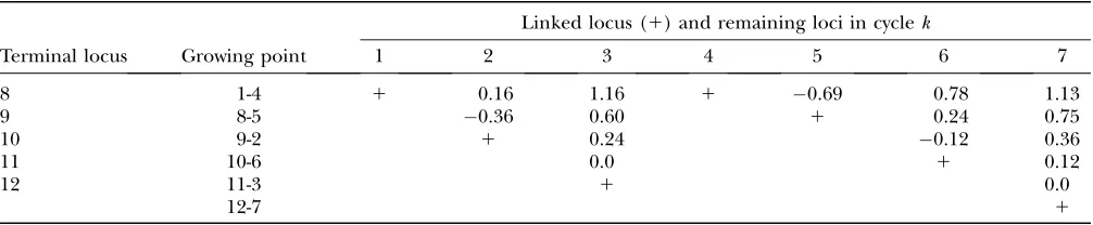
We first illustrate the UG algorithm using a hypothetic data set (see Table 1) that was generated from the map (1-4-5-2-6-3-7) in which all the loci are codominant and the distances between adjacent loci are all 10 cM. As the algorithm indicates, the first step is to find a terminal map through Equation 3. It turns out that T14 is (see Table 2) the smallest T-value (below the diagonal in Table 2). Therefore according to the algorithm the terminal map is 1-4, which is also designated as composite locus 8. After computing the distance be-tween locus 8 and each of the remaining simple loci using Equation 7, it is found from Table 3 and Equation 8 that locus 5 is the next locus to be added to the map. Sinced54¼0.1,d51¼0.22, the map grows into 1-4-5, which is designated as locus 9. This completes step 1 of the algorithm. In the second step,d9i (i¼2, 3, 6, 7) is
computed using Equation 9, and in the third stepH9iis
computed using Equation 10. It turns out thatH92is the smallest (see Table 3), which leads to the partial map 1-4-5-2, which is designated as locus 10. Repeating steps 2 and 3, it is found in Table 3 that the next locus to be
added is locus 6, then locus 3, and finally locus 7. The complete map is thus estimated to be 1-4-5-2-6-3-7, which is the same as the true map.
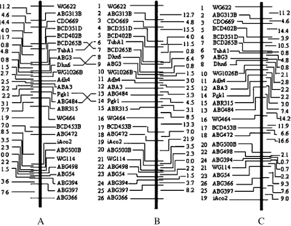
To see how the UG algorithm performs in reality, we applied it to a real data set of 26 loci on barley chromosome I from the North American Barley Ge-nome Mapping Project (see Liu1998, p. 288). For the
purpose of comparison, we applied both the UG and the NM algorithms to this data set, which yielded maps A and C, respectively, in Figure 2. Also included is the map (B) based on 1000 bootstrap samples from Liu(1998,
p. 297) in statistical genomics-linkage, mapping, and QTL analysis. It is obvious that maps A and B are almost identical. The only notable difference is the positions of three pairs of loci. For the given observed data set, map A appears to be reasonable because the recombination fraction between loci BCD265B and Dhn6 is 7.97, which is larger than those between loci TubA1 and BCD265B (0.75) and between TubA1 and ABG3 (4.8). A similar situation also occurs among loci ABA3, ABG484, Pgk1, and ABR315. In comparison, there are considerable differences between maps B and C. It is noteworthy that sums of adjacent distances on linkage maps A, B, and C are, respectively, 132.8, 148.5, and 151 cM, which sug-gests that linkage map A is the best among these three linkage maps according to the principle of minimum SARF (Falk1992; Liu1998).
PERFORMANCE OF THE UG ALGORITHM
Since few real data sets are available with known maps of the loci involved, we use computer simulation to generate data so that the performance of the UG algorithm can be compared to those of some widely used approaches such as NM, SA, SA-Opt2, and ES-2Opt (Mester et al. 2003). Although we carried out many
comparisons, we present some representative results only for four numbers of codominant loci: 6, 30, 50, and 100. The latter two cases represent relatively large maps. For each number of loci, two types of map are considered. The first one is an equal distance (ED) map in which all recombination distances between adjacent loci are set to be 10 cM. The second one is a random distance (RD) map in which the distance between the adjacent loci is set to be a value randomly selected from the five possible values: 10, 15, 20, 25, and 30 cM.
The simulation starts with two isogenic lines, repre-senting the paternal and maternal lineages, respectively. We employed the point process model by Foss et al.
(1993) in our simulations. For each meiosis resulting in the F1individuals, recombination events are assumed to occur between two adjacent loci with a certain proba-bility that is proportional to the distance (in centimor-gans). We considered both the presence and the absence of recombination interference. In the case of no interference, recombination between each pair of Figure1.—An example of a linkage map of four linked loci
in which there are three adjacent intervals (1-2, 2-3, and 3-4) and three nonadjacent intervals (1-3, 2-4, and 1-4).
TABLE 1
Recombination fractions between loci of the linkage map 1-4-5-2-6-3-7, where each of the adjacent intervals was
assigned to be 10 cM
Locus
Locus 1 2 3 4 5 6
2 0.30
3 0.49 0.20
4 0.10 0.20 0.40
5 0.20 0.10 0.30 0.10
6 0.40 0.10 0.10 0.30 0.20
adjacent loci is independently simulated between any two nonsister chromatids (Weinstein1936) with equal
probability and proceeds without chromatid interfer-ence (Fosset al. 1993). For the case of interference, we
considered only an extreme situation, which is a com-plete interference. In such a case, a crossover in a particular interval between two nonsister chromatids cannot occur when there is already a crossover in an interval within 30 cM.
The F2generation is simulated by crossing the indi-viduals of the F1generation. The ratio of the paternal homozygotes, heterozygotes, and maternal homozy-gotes among F2individuals is expected to be 1:2:1. To mimic the practice in a typical crossing experiment, we retain the sample of F2individuals only when the ratio does not significantly deviate from 1:2:1. Once the sample of F2individuals is obtained, the EM algo-rithm (see, for example, Liu1998) is used to estimate
the recombination fraction (r) between each pair of loci.
Since our main purpose is to recover the correct map, we measure the performance of a method by its success rate of recovering the true map to a given extent. Most important is whether a method is capable of completely recovering the true map. In all our results, we found that distance defined by Equation 13 performs slightly better than that defined by Equation 11; therefore, we report only the results based on the distance defined by Equation 13. Table 4 shows the results for the five methods for complete recovery of the map with six
codominant loci. It is clear that the SA algorithm has almost no chance of recovering the true map, which agrees with the finding by Stam(1993). However, the
combination of SA with the 2Opt optimization pro-cedure (Linand Kernighan1973) improves it
consid-erably, although it is still a poor performer. The ES-2Opt is overall more efficient than the SA-2Opt, particularly with large sample sizes. The performance of the NM algorithm is good overall except for the case of in-terference with equal distance between adjacent loci.
Among the five methods compared, the UG algo-rithm is clearly the most efficient method; its improve-ment in efficiency over the other four methods is particularly profound when the sample size is small. For example, for a sample of 50 individuals, the UG algorithm has a 76–87% efficiency while the best of the other four methods achieves only 49% efficiency.
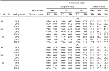
Since overall the NM is the best among the existing methods, we carried out more extensive comparisons between the performances of the NM and the UG. In addition to the complete recovery, it is also informative to see if a method can recover most of the true map, for example, recovering 90% of a true map. Table 5 shows the efficiencies of the NM method and the UG method in recovering several percentages of the true map in the cases of 30, 50, and 100 codominant loci. In the case of no interference, the efficiencies of both methods grow as sample size increases, but in any sample size the UG method greatly outperforms the NM method. In partic-ular, the UG method is weakly sensitive to sample size. TABLE 2
Distances (above diagonal) andT-values (below diagonal) for the seven loci specified in Table 1
Locus
Locus 1 2 3 4 5 6 7
1 0.34 0.59 0.10 0.22 0.47 0.64
2 2.9959 0.22 0.22 0.10 0.10 0.34
3 2.9925 2.6967 0.47 0.34 0.10 0.10
4 3.9725 2.6967 2.7000 0.10 0.34 0.59
5 3.3625 2.5667 2.5833 3.0633 0.22 0.47
6 2.8692 2.5667 3.0633 2.5833 2.4533 0.22
7 3.4333 2.9959 3.9725 2.9925 2.8692 3.3625
TABLE 3
UG procedure for mapping the seven loci
Linked locus (1) and remaining loci in cyclek
Terminal locus Growing point 1 2 3 4 5 6 7
8 1-4 1 0.16 1.16 1 0.69 0.78 1.13
9 8-5 0.36 0.60 1 0.24 0.75
10 9-2 1 0.24 0.12 0.36
11 10-6 0.0 1 0.12
12 11-3 1 0.0
For example, in the samples of 100, 200, and 300 F2 individuals, the UG method has, respectively, 74, 86, and 88% accuracies to completely recover the true map of 100 1oci of RD and 82, 98, and 100% accuracies to completely recover the true map of 100 loci of ED. In comparison the NM method has only, respectively, 15, 30, and 31% accuracies for recovering the RD map and 22, 70, and 79% for recovering the ED map. On the other hand, it is also seen from Table 5 that, in com-parison with the NM method, the UG method does not obviously tend to perform poorly as the number of linked loci increases and its mapping efficiency is not significantly affected by crossover interference.
DISCUSSION
As pointed out in the Introduction, several principles can be used to reconstruct linkage maps. The SA, SA-2Opt, and ES-2Opt are methods aimed at minimizing
the sum of adjacent recombination fractions or adjacent distances in the linkage map. This minimization princi-ple is correct in theory but often does not work well in practice due to various types of random errors. Indeed, even with exactly the same linkage map for all the individuals subjected to the experiment, the observed recombination fractions may fluctuate widely from experiment to experiment due to sampling variation, ecological condition, sex, genotype, and age (Mester
et al. 2003). Therefore, the estimated linkage map based
on the minimization principle is often poor quality. The NM method is based on the neighbor joining of Saitou
and Nei (1987). Since its search criteria closely mimic
the minimization principle, the overall accuracy of the NM method is similar to the best in the class of methods based on the minimization principle.
The UG algorithm does not rely on the minimization principle, yet achieves higher accuracy in recovering the true map. Theorem 1 apparently is the foundation for Figure 2.—Comparison among three linkage
maps. Maps A and C were estimated using the UG and NM methods, respectively, on the basis of a recombination fraction data set of 26 loci from Liu (1998) and map B was from Liu
(1998), which was based on 1000 bootstrap samples.
TABLE 4
The efficiencies of different map-making methods in complete recovery of the true map with six codominants
Distance status
ED RD
Crossover status: Independence Interference Independence Interference
Sample size: 50 300 50 300 50 300 50 300
SA 0.0 0.0 0.0 1.0 2.0 0.0 2.0 0.0
SA-2Opt 21.0 33.0 38.0 37.0 25.0 39.0 29.0 37.0
ES-2Opt 36.0 58.0 41.0 63.0 46.0 60.0 49.0 62.0
NM 31.0 79.0 20.0 25.0 39.0 93.0 36.0 89.0
UG 87.0 100.0 84.0 100.0 82.0 100.0 76.0 100.0
its success, which indicates that there is a high proba-bility that the terminal loci of the true map can be identified through utilization of distances among mul-tiple loci simultaneously. Although the theorem is proven only for strictly additive distance, the fact that the UG algorithm works very well with distances defined either as the estimated recombination fractions or as the corrected estimates indicates that Equation 3 is robust against modest deviation by the distance from strict additivity. This pleasing result appears because the loci critical for determining the status of a particular locus are those nearby, whose distance to the given locus is likely more additive than that of those far away. In addition to its high accuracy, the UG algorithm also has the advantage of speed, particularly when the number of loci is large, compared with the NM algorithm. This is because it takesn1 cycles to complete while the NM algorithm takesn(n 1)/2 cycles. Therefore, the UG algorithm should be a useful addition to the tools for large-scale linkage mapping and for evaluating the confidence of the estimated map by bootstrap or jackknife (Liu1998; Mesteret al. 2003).
We thank the High Performance Computer Center of Yunnan University for computational support and Sara Barton for editorial assistance. This work was partly supported by National Institutes of Health grant R01 GM50428 and funds from Yunnan University.
LITERATURE CITED
Buetow, K. N., and A. Chakravarti, 1987 Multipoint gene
map-ping using seriation. Am. J. Hum. Genet.41:189–201. Echt, C., S. Knappand B.-H. Liu, 1992 Genome mapping with
non-inbred crosses using GMendel 2.0. Maize Genet. Coop. Newsl.66:
27–29.
Edwards, J. H., 1971 The analysis of X-linkage. Ann. Hum. Genet.
34:229–250.
Ellis, T. H. N., 1997 Neighbor mapping as method for ordering
genetic markers. Genet. Res.69:35–43.
Eppig, J., and E. M. Eicher, 1983 The mouse linkage map. J. Hered.
74:213–231.
Falk, C. T., 1992 Preliminary ordering of multiple linked loci using
pairwise linkage data. Genet. Epidemiol.9:367–375.
Foss, E., R. Lande, F. W. Stahland C. M. Steinberg, 1993 Chiasma
interference as a function of genetic distance. Genetics133:681– 691.
Haldane, J. B. S., 1919 The combination of linkage values and the
calculation of distances between the loci of linked factors. J. Genet.8:299–309.
Jensen, J., and J. H. Jorgensen, 1975 The barley chromosome 5
linkage map. Hereditas80:5–16.
Knapp, M., M. Neugebauer, R. Fimmers, S. A. Seuchterand M. P.
Baur, 1989 Preliminary ordering of multipoint linkage data,
pp. 41–46 inMultipoint Mapping and Linkage Based Upon Affected Pedigree Members (Genetic Analysis Workshop), edited by R. C. Elston, M. A. Spence, S. E. Hodgeand J. W. MacCluer. Alan
R. Liss, New York.
Kosambi, D. D., 1944 The estimation of map distances from
recom-bination values. Ann. Eugen.12:172–175.
Lander, E. S., and P. Green, 1987 Construction of multilocus
link-age maps in human. Proc. Natl. Acad. Sci. USA84:2363–2367. Lander, E. S., P. Green, J. Abrahamson, A. Barlow, M. J. Daly
et al., 1987 MapMaker: an interactive computer package for
TABLE 5
Comparison between UG and EM methods in their accuracies of partially (80%, 90%) and completely (100%) recovering the model linkage maps of 30, 50, and 100 codominant loci
Crossover status
Independence Interference
Sample size: 100 200 300 100: 200: 300:
Loci Recovering mode Distance status: ED RD ED RD ED RD RD RD RD
NM
30 80% 86.0 61.0 99.0 86.5 100.0 87.0 69.0 84.0 89.0
90% 86.0 60.0 98.0 86.5 100.0 87.0 66.0 84.0 89.0 100% 85.0 59.0 98.0 86.0 100.0 86.0 63.0 84.0 89.0
50 80% 74.0 39.0 95.0 64.0 100.0 70.0 42.0 63.3 73.0
90% 65.0 37.0 95.0 64.0 100.0 70.0 35.5 60.7 73.0 100% 63.0 36.0 95.0 64.0 100.0 70.0 34.5 59.7 72.7
100 80% 39.0 17.0 71.0 33.0 79.0 33.0 13.1 33.0 39.3
90% 32.0 16.0 71.0 31.0 79.0 32.0 10.7 32.0 39.3 100% 22.0 15.0 70.0 30.0 79.0 31.0 7.1 32.0 39.3
UG
30 80% 98.0 92.0 100.0 98.0 100.0 98.5 93.0 98.0 99.0 90% 98.0 92.0 100.0 98.0 100.0 98.5 92.0 98.0 99.0 100% 95.0 92.0 100.0 98.0 100.0 98.5 92.0 98.0 99.0 50 80% 96.0 88.0 100.0 92.0 100.0 97.0 91.0 98.0 98.0 90% 96.0 88.0 100.0 92.0 100.0 97.0 90.0 98.0 98.0 100% 95.0 87.0 100.0 92.0 100.0 97.0 85.5 98.0 98.0 100 80% 92.0 88.9 99.0 88.0 100.0 89.0 92.9 97.8 98.9 90% 92.0 85.6 99.0 86.0 100.0 89.0 89.3 97.8 98.9 100% 82.0 74.4 98.0 86.0 100.0 88.0 81.0 97.8 97.8
constructing genetic linkage maps of experimental and natural populations. Genomics1:174–181.
Lathrop, G. M., J. M. Lalouel, C. Julierand J. Ott, 1984
Strat-egies for multilocus linkage analysis in human. Proc. Natl. Acad. Sci. USA81:3443–3446.
Lathrop, G. M., J. M. Lalouel, C. Julierand J. Ott, 1985 Multilocus
linkage analysis in humans: detection of linkage and estimation of recombination. Am. J. Hum. Genet.37:482–498.
Lin, S., and B. Kernighan, 1973 An effective heuristic algorithm for
the TSP. Oper. Res.21:498–516.
Liu, B.-H., 1998 Statistical Genomics: Linkage, Mapping, and QTL
Anal-ysis. CRC Press, New York.
Lu, Y. Y., and B. H. Liu, 1995 PGRI, a software for plant genome
research. Plant Genome III. Abstract, January, 1995, San Diego. Mester, D., Y. Ronin, D. Minkov, E. Nevo and A. Korol,
2003 Constructing large-scale genetic maps using an evolution-ary strategy algorithm. Genetics165:2269–2282.
Olson, J. M., and M. Boehnke, 1990 Monte Carlo comparison of
preliminary methods of ordering multiple genetic loci. Am. J. Hum. Genet.47:470–482.
Saitou, N., and M. Nei, 1987 The neighbor-joining method: a new
method for reconstructing phylogenetic tree. Mol. Biol. Evol.4:
406–425.
Stam, P., 1993 Construction of integrated genetic linkage maps
by means of a new computer package: JoinMap. Plant J.3:739– 744.
Suiter, K. A., J. F. Wendel and J. Case, 1983 SLINKAGE-1: a
PASCAL computer program for the detection and analysis of ge-netic linkage. J. Hered.74:203–204.
Thompson, E. A., 1984 Information gain in joint linkage analysis.
IMA J. Math. Appl. Med. Biol.1:31–49.
Weeks, D., and K. Lange, 1987 Preliminary ranking procedures for
multilocus ordering. Genomics1:236–242.
Wilson, R. S., 1988 A major simplification in the preliminary
order-ing of linked loci. Genet. Epidemiol.5:75–80.
Weinstein, A., 1936 The theory of multiple-strand crossing over.
Genetics21:155–199.
Communicating editor: N. Takahata
APPENDIX A
Proof of Theorem1. For additive distance,Si(i,n) can be written as
Si¼
Xi1
k¼1
kdkk111 Xn1
k¼i
ðnkÞdkk11¼ Xi
k¼1
kdkk111ðn2iÞdii111 Xn1
k¼i11
ðnkÞdkk11¼Si111ðn2iÞdii11:
Forj.n=2,i.e., the largest integer#n/2, we have
TijTij11¼2dijSj2ðdij1djj11Þ1Sj11 ¼ 2djj11Sj11 ðn2jÞdjj111Sj11¼ ½2ðj1Þ ndjj11$0 and fori$n=2
TijTi11j¼2dijSi2di11j1Si11¼2dii11Si11 ðn2iÞdii111Si11¼ ð2inÞdii11$0:
Similarly for i,n=2, Ti1jTij#0 and for j$n=2, Tij1Tij#0. It thus follows that when i$n=2 we have Tij$Tin$Tn1nand whenj#n=2 we haveT12#T1j#Tij. Finally wheni,n=2 andj.n=2, we haveTij$T1j$T1n.
n
Furthermore we have
1
2ðT121Tn1nÞ T1n ¼d121dn1n ðððn12Þ=2Þd121nd231 1ndn2n11ððn12Þ=2Þdn1nÞ 2d1n1ðnd121nd231 1ndn2n11ndn1nÞ
¼ ððn=2Þd121n2dn1nÞ 2d1n¼nðd121dn1nÞ=22d1n:
APPENDIX B
Proof of Theorem2. Using the recurrence equation forSi fromappendix a, we have
H1iH1i11 ¼ ðn1Þd1iSi ðn1Þd1i111Si11¼ ðn1Þdii11 ðn2iÞdii11¼ ð2n2i1Þdii11#0 fori#n1. It is clear that comparison betweenH1iandH1i11leads to