Packet Aggregation Based Backpressure Scheduling in Multi-hop Wireless Networks.

(1)

ABSTRACT

DEUSKAR, GAURISH CHANDRASHEKHAR. Packet Aggregation based Backpressure Scheduling in Multi-hop Wireless Networks. (Under the direction of Dr. Rudra Dutta.)

(2)

Packet Aggregation based Backpressure Scheduling in Multi-hop Wireless Networks

by

Gaurish Chandrashekhar Deuskar

A thesis submitted to the Graduate Faculty of North Carolina State University

in partial fulfillment of the requirements for the Degree of

Master of Science

Computer Science

Raleigh, North Carolina

2010

APPROVED BY:

Dr. George Rouskas Dr. Injong Rhee

(3)

DEDICATION

(4)

BIOGRAPHY

(5)

ACKNOWLEDGEMENTS

I would like to thank my advisor, Dr. Rudra Dutta for advising me in this study. I am grateful to him for his valuable ideas and insights in various directions. I also thank him for helping me in domains other than my research like giving me more disk space for my simulations.

I would also like to thank Dr. George Rouskas and Dr. Injong Rhee for agreeing to be on my committee.

I would also like to thank my room mate Parth Pathak for his help in solving my doubts in this thesis.

(6)

TABLE OF CONTENTS

List of Tables . . . vii

List of Figures . . . .viii

Chapter 1 Introduction . . . 1

1.1 Background and challenges . . . 1

1.2 Motivation . . . 2

1.3 Organization . . . 3

Chapter 2 Related work . . . 4

2.1 Work on backpressure scheduling and congestion control . . . 4

2.2 Work on packet aggregation . . . 6

Chapter 3 Packet aggregation with PDQ scheduling . . . 8

3.1 Terms . . . 8

3.1.1 Per Destination Queues (PDQ) . . . 8

3.1.2 Urgency weight . . . 8

3.1.3 Urgency Weight state (UW state) . . . 8

3.1.4 MAC priorities . . . 9

3.1.5 Packet aggregate . . . 9

3.2 Methodology . . . 10

3.2.1 Basic idea . . . 10

3.2.2 Aggregation process . . . 10

3.2.3 De-aggregation process . . . 11

3.3 Example . . . 11

3.4 Theoretical analysis . . . 15

3.4.1 Terms . . . 15

3.4.2 Modelling average throughput of a flow . . . 17

3.4.3 Modelling the buffer process . . . 19

Chapter 4 Experimental methodology: OPNET simulation . . . 21

4.1 Requirements . . . 21

4.2 OPNET basics . . . 21

4.2.1 Node model . . . 21

4.2.2 Process Model . . . 22

4.3 UW header . . . 23

4.4 Changes in the wlan process model . . . 24

4.4.1 Event: Packet arrival from higher layer . . . 24

4.4.2 Event: Packet transmission . . . 24

(7)

Chapter 5 Experimental methodology: Linux kernel implementation . . . 29

5.1 Linux network stack overview . . . 29

5.1.1 Thesk buff structure . . . 29

5.1.2 Packet transmission overview . . . 29

5.1.3 Packet reception overview . . . 31

5.2 Netfilter architecture . . . 33

5.3 Madwifi driver . . . 33

5.4 Implementation details . . . 34

5.4.1 Per-destination queues and netfilter-specific code . . . 34

5.4.2 Scheduler . . . 35

5.4.3 Promiscuous handler . . . 35

5.4.4 Aggregation . . . 36

Chapter 6 Experimental set-up and numerical results . . . 38

6.1 Metrics of interest . . . 38

6.2 OPNET simulations . . . 39

6.2.1 Parameters . . . 40

6.3 Linux testbed results . . . 66

Chapter 7 Summary and future work . . . 67

(8)

LIST OF TABLES

Table 5.1 Values of 802.11e parameters for different priority levels . . . 34

(9)

LIST OF FIGURES

Figure 1.1 Throughput of different packet sizes . . . 2

Figure 3.1 Format of a packet aggregate . . . 9

Figure 3.2 PDQ scheduling without aggregation . . . 13

Figure 3.3 PDQ scheduling with aggregation . . . 14

Figure 4.1 OPNET node model wlan wkstn adv . . . 22

Figure 4.2 OPNET process model wlan proc . . . 23

Figure 4.3 UW header format . . . 24

Figure 4.4 Enqueue flowchart . . . 26

Figure 4.5 Dequeue flowchart . . . 27

Figure 4.6 Dequeue flowchart with Aggregation . . . 28

Figure 5.1 Linux kernel packet transmission . . . 30

Figure 5.2 Linux kernel packet reception . . . 31

Figure 5.3 Netfilter hooks . . . 32

Figure 6.1 Grid topology (49 nodes) . . . 41

Figure 6.2 Clustered topology (36 nodes) . . . 41

Figure 6.3 Random topology 1 (25 nodes) . . . 42

Figure 6.4 Random topology 2 (16 nodes) . . . 42

Figure 6.5 Aggregate Throughput (Random topology 1, 11 Mbps channel rate, ex-ponential distribution) . . . 44

Figure 6.6 Aggregate Throughput (Random topology 1, 1 Mbps channel rate, expo-nential distribution) . . . 44

Figure 6.7 Network utility (Random topology 1, 11 Mbps channel rate, exponential distribution) . . . 45

Figure 6.8 Network utility (Random topology 1, 1 Mbps channel rate, exponential distribution) . . . 45

Figure 6.9 Fairness Index (Random topology 1, 11 Mbps channel rate, exponential distribution) . . . 46

Figure 6.10 Fairness Index (Random topology 1, 1 Mbps channel rate, exponential distribution) . . . 46

Figure 6.11 Average buffer occupancy (Random topology 1, 11Mbps channel rate, 4 flows, exponential distribution) . . . 47

Figure 6.12 Average buffer occupancy (Random topology 1, 11Mbps channel rate, 8 flows, exponential distribution) . . . 47

(10)

Figure 6.15 Average buffer occupancy (Random topology 1, 1 Mbps channel rate, 8 flows, exponential distribution) . . . 49 Figure 6.16 Average buffer occupancy (Random topology 1, 1 Mbps channel rate, 12

flows, exponential distribution) . . . 49 Figure 6.17 Average buffer occupancy (Random topology 1, 1 Mbps channel rate, 16

flows, exponential distribution) . . . 50 Figure 6.18 Aggregate throughput simulated vs theory (Random topology 1, 11 Mbps

channel rate, exponential distribution) . . . 50 Figure 6.19 Average network delay (Random topology 1, 11 Mbps channel rate,

ex-ponential distribution) . . . 51 Figure 6.20 Random topology 1, 11 Mbps channel rate, exponential distribution,

50-60 percent medium utilization . . . 51 Figure 6.21 Random topology 1, 1 Mbps channel rate, exponential distribution, 50-60

percent medium utilization . . . 51 Figure 6.22 Aggregate throughput (Cluster topology, 11 Mbps channel rate,

exponen-tial distribution) . . . 52 Figure 6.23 Network utility (Cluster topology, 11 Mbps channel rate, exponential

dis-tribution) . . . 52 Figure 6.24 Fairness index (Cluster topology, 11 Mbps channel rate, exponential

dis-tribution) . . . 53 Figure 6.25 Average buffer occupancy (Cluster topology, 11 Mbps channel rate, 4

flows, exponential distribution) . . . 53 Figure 6.26 Average buffer occupancy (Cluster topology, 11 Mbps channel rate, 8

flows, exponential distribution) . . . 55 Figure 6.29 Aggregation opportunities (Cluster topology, 11 Mbps channel rate,

ex-ponential distribution) . . . 55 Figure 6.30 Average network delay (Cluster topology, 11 Mbps channel rate,

expo-nential distribution) . . . 56 Figure 6.31 Aggregate throughput (Grid topology, 11 Mbps channel rate, exponential

distribution) . . . 56 Figure 6.32 Network utility (Grid topology, 11 Mbps channel rate, exponential

distri-bution) . . . 57 Figure 6.33 Fairness Index (Grid topology, 11 Mbps channel rate, exponential

distri-bution) . . . 57 Figure 6.34 Average network delay (Grid topology, 11 Mbps channel rate, exponential

distribution) . . . 58 Figure 6.35 Average buffer occupancy (Grid topology, 11 Mbps channel rate,

expo-nential distribution) . . . 58 Figure 6.36 Aggregation opportunities (Grid topology, 11 Mbps channel rate,

(11)

Figure 6.37 Aggregate throughput (Grid topology, 11 Mbps channel rate, exponential distribution, internet packet sizes) . . . 59 Figure 6.38 Network utility (Grid topology, 11 Mbps channel rate, exponential

distri-bution, internet packet sizes) . . . 60 Figure 6.39 Fairness index (Grid topology, 11 Mbps channel rate, exponential

distri-bution, internet packet sizes) . . . 60 Figure 6.40 Average network delay (Grid topology, 11 Mbps channel rate, exponential

distribution, internet packet sizes) . . . 61 Figure 6.41 Average buffer occupancy (Grid topology, 11 Mbps channel rate,

expo-nential distribution, internet packet sizes) . . . 61 Figure 6.42 Aggregation opportunities (Grid topology, 11 Mbps channel rate,

expo-nential distribution, internet packet sizes) . . . 62 Figure 6.43 Aggregate throughput (Random topology 2, 11 Mbps channel rate,

expo-nential distribution) . . . 62 Figure 6.44 Network utility (Random topology 2, 11 Mbps channel rate, exponential

distribution) . . . 63 Figure 6.45 Fairness Index (Random topology 2, 11 Mbps channel rate, exponential

distribution) . . . 63 Figure 6.46 Average buffer occupancy per node (Random topology 2, 11 Mbps channel

rate, exponential distribution) . . . 64 Figure 6.47 Average network delay (Random topology 2, 11 Mbps channel rate,

ex-ponential distribution) . . . 64 Figure 6.48 Aggregate throughputs (Random topology 2, 4 flows, Different channel

(12)

Chapter 1

Introduction

1.1 Background and challenges

(13)

0

5

10

15

20

25

30

35

40

0 200 400 600 800 1000 1200 1400 1600

Throughput (Mbps)

aggregation

regular

Figure 1.1: Throughput of different packet sizes

1.2 Motivation

Surveys on the wide area traffic patterns have shown that majority of the wide area internet traffic has small packet sizes [16, 29]. Also, in the last mile wireless networks, a considerable amount of traffic is formed of small packet sizes. [26] and [22] show that about 70 to 80 percent of the overall application level traffic has packet sizes less than 100 bytes. This is because applications like chat, web requests, ssh traffic, Kerberos, ICMP, DNS, BOOTP contribute to small packet sizes. The problem with small packet sizes is the overhead associated with them due to the PLCP, MAC header, trailers and contention time which almost increases exponentially with the number of wireless nodes in a collision domain. [14] shows that for a TCP acknowledgement of size 40 bytes, about 90 percent overhead is associated when 802.11b with 11M channel rate is used. With the higher percentage of small packet sizes and with the multi-hop scenario, it is evident that the overall network utilization would be much less owing to the huge overheads. Thus the idea of packet aggregation at the IP level is considered (multiple IP packets are aggregated into one single IP packet which then becomes the MAC SDU).

(14)

are packed into one single MAC SDU. Iperf was run between 2 machines with one wireless card on each of those machines set at 54Mbps channel rate, 11g MAC. It can be seen that for small packet sizes, the flow with aggregation receives more throughput than the flow with no aggregation. We can thus say that aggregation causes an increase in the service rate achieved by a flow.

The central principle of studies of cross layer approach to scheduling like [6] and [30] is to introduce differentiated service rate at the MAC layer based on the amount of backpressure of per-destination queues. They achieve this by the help of differentiated access to the medium. We investigate in our study whether we can combine such backpressure based PDQ mechanisms with packet aggregation technique to get at least some benefit out of aggregation in terms of the aggregate throughput while preserving the important benefit of PDQs which is fairness and congestion control. In this thesis, we use packet aggregation as a tool to introduce MAC layer service differentiation: queues with more back pressure have more opportunity for packet aggregation thereby increasing their service rate. Using our design of PDQ+Aggregation which will be described in later sections, we see that for small packet sizes we increase the aggregate throughput of the network while preserving fairness amongst flows. Also, in some cases, we actually get better fairness along with good aggregate throughput.

1.3 Organization

(15)

Chapter 2

Related work

2.1 Work on backpressure scheduling and congestion control

The problem of scheduling involves determining which packet from a node is to be transmitted the next and also which link among a set of interfering links is to be scheduled the next. The problem of congestion control involves maintaining the source rate control meaning at each time step whether a packet should be added to a flow at the source node. The aim of both of these problems is to get good throughput and fairness across different flows in the network. Much of the previous research has considered these two problems separately. Kelly, Mauloo and Tan [15] addressed the issue of congestion control and have not looked at how data is scheduled. They tried to solve the congestion control problem as a distributed optimization problem, by formulating it as the classic Network Utility Modelling problem in the context of wireless networks defined below; where the utility functions Uf assigned to flows reflect the

desire of the network as a whole to minimize congestion.

Maximize:X

f

Uf(xf)

subject to:

X

f∈Se

xf ≤ce

where Se are the set of flows passing through servere,xf is the current injection rate into

flowf and ce is the capacity of each server.

(16)

of per destination queues (PDQs) at each node in the network. These queues contain the packets destined to their respective destination. They also have the notion of urgency weights associated with it. The urgency weight of a PDQ is equal to the backlog of the queue minus the backlog of the PDQ of the next hop towards the destination. Also both of these studies employ a MAC providing differentiated service meaning that it is possible to provide different levels of MAC layer throughputs across different traffic flows. The MAC scheduling happens thusly:

1. Each node maintains a “urgency weight context” of the neighbourhood which contains the urgency weight information of the PDQs of the nodes in the neighbourhood.

2. When the next packet is to be transmitted, it is chosen from the PDQ with the highest urgency weight and is the head of line packet

3. The packet is transmitted with a MAC layer priority depending upon the urgency weight of its PDQ and the “urgency weight context”

[6] chooses the MAC layer priority of the packet by changing the value of CWmin which is specified by the 802.11 standard. Those packets which are from higher urgency weight PDQs take a low value of CWmin thereby increasing their chance of medium access quickly in the neighbourhood whereas those packets which come from lower urgency weight PDQs take a high value of CWmin thereby decreasing their chance of quickly accessing the medium. With respect to congestion control, this work uses a utility based congestion control. Each flow is assigned a log based utility where the utility or the “benefit” a flow provides to the system or the network as a whole is equal to the log of the current throughput received by that flow. The congestion control mechanism operates at the source node where the flow originates and is performed accordingly:

A packet from the source node is added to the PDQ only if it satisfies the following equation.

U0(x)> β∗q (2.1)

where β is a small constant and ‘q’ is the size of the respective PDQ. While [6] have simulated in OPNET [1]; [30] have implemented PDQ scheduling and congestion control in the Linux kernel. This work does the differentiated MAC layer scheduling using the IEEE 802.11e [21] mechanism. They have 4 levels of service at the MAC layer implemented in the modified madwifi driver. A packet to be transmitted is mapped to the appropriate service level based on its urgency weight.

(17)

Algorithm 1 AIMD source rate control if qlen≥QU EU E T HRESH then

rate←rate/β else

rate←rate+α end if

where QUEUE THRESH,α and β are constants and rate is the rate of the flow.

Solutions of [6] and [30] have shown to solve the problem of starvation of flows, provide better fairness and increase the network utility.

2.2 Work on packet aggregation

Aggregation can be performed at different layers: The MAC layer where it is called frame aggregation, the IP layer and even at the transport layer. Packets that are aggregated at a given layer share common headers of the layers below it. [11, 14, 18, 23, 24, 32], etc. belong to the category where packets are aggregated at the IP layer. Thus multiple IP packets go into the same MAC frame. On the other hand, aggregation which is performed at the MAC layer which is also called as frame aggregation has been experimented in [13, 17].

Aggregation can also be classified as hop by hop and end to end. In the end to end case, packets are aggregated at the source node itself and the aggregated packets then travel as it is to the destination. [11, 23] are examples of such a case. This introduces less aggregation opportunities at the intermediate nodes. [14] is an example of packet aggregation for the hop to hop case. Aggregation can also be classified as forced delay based or no-delay based. In the forced delay based aggregation packets are forced to wait for some time so that new packets are available for aggregation thereby increasing the aggregation opportunities. This kind of aggregation should be designed carefully as it might cause unnecessary delays which may be bad for applications like VoIP. [11, 14, 23] introduce forced delay based aggregation.The choice of optimal packet size for aggregation is also one of the important design parameters for getting good throughput in the face of noise. [23] uses the WCETT [20] metric of the path for choosing the maximum packet size of the aggregated packet that is transferred across that path. WCETT of a path from a source to destination is defined as the weighted sum of the sum of the ETTs (Expected transmission time) of links on that path and the largest ETT on that path.

(18)

reduce the energy consumption but to alleviate the congestion in the network. In that network, the authors use special type of nodes which are called “aggregator” nodes which are dedicated to perform aggregation. In contrast to this, the work in this report does not have special “ag-gregator” node but instead any node can perform aggregation if it is eligible to do so.

In this thesis, aggregation is done on a per destination basis on each hop independently. In section 3.3, we give an example which describes our strategy of packet aggregation wherein the PDQ having the highest urgency weight in the neighborhood gets chance to aggregate packets upto the point where it remains the highest urgency weight PDQ.

(19)

Chapter 3

Packet aggregation with PDQ

scheduling

3.1 Terms

In this section we will gloss over the important terms and their meanings used in the thesis.

3.1.1 Per Destination Queues (PDQ)

Each node maintains a separate queue for every possible destination in the network. The traffic that the node generates or forwards to a destination goes into the the PDQ for that destination.

3.1.2 Urgency weight

Every PDQ has an urgency weight associated with it. The urgency weight is equal to the backlog of the PDQ subtracted by the backlog of the PDQ on the next hop node towards the destination. The urgency weight information is used by the works [6] and [30] for back-pressure scheduling.

3.1.3 Urgency Weight state (UW state)

(20)

IP Data 1 IP Data 2

••• IP Data n

Figure 3.1: Format of a packet aggregate

2. The PDQ ID, node ID and urgency weight of the PDQ having maximum urgency weight in the neighborhood

3. The PDQ ID, node ID and urgency weight of the PDQ having minimum urgency weight in the neighborhood

With the help of this information, a node determines the MAC priority of the next packet to be transmitted. How to maintain the UW state is explained in subsequent chapters 4 and 5.

3.1.4 MAC priorities

It is assumed that the MAC layer is able to provide different levels of service. In our experiments, 4 MAC priorities are considered: 0, 1, 2, and 3. 3 is the highest priority while 0 is the lowest. With a CSMA/CA kind of MAC which is considered in our experiments, when a packet is transmitted with priority 3, it has higher probability of accessing the medium while a packet with priority 0 has a lower probability of accessing the medium. With a regular 802.11 MAC, priority 3 means choosing the backoff with a low value of CWmin. This is used in OPNET simulations. With the 802.11e MAC, priority 3 means having lower values of AIFS, CWmin and CWmax. This is used in the linux kernel experiments. On a node, the next packet to be transmitted is chosen as the head of line (HOL) packet from the PDQ having the highest urgency weight. This is the intra-node scheduling. The MAC priority with which the packet is transmitted is chosen linearly from the range 0-3 by mapping the urgency weight of the PDQ to which the packet belongs to the range

{minimum urgency weight in the neighborhood, maximum urgency weight of the neighborhood}

It follows that if the PDQ from which the packet is to be transmitted has the highest urgency weight in the neighborhood, then the packet will be transmitted with priority 3 whereas if the PDQ has the lowest urgency weight in the neighborhood, then the packet will be transmitted with priority 0.

3.1.5 Packet aggregate

(21)

aggregate. Its format is shown in figure 3.1. What contains in the aggregation header is explained in chapters 4 and 5.

3.2 Methodology

3.2.1 Basic idea

The idea of backpressure scheduling is to give more service rate to queues having higher urgency weight. With the help of aggregation, multiple packets from the same PDQ (per destination queue) with the highest urgency weight are aggregated together. Due to this, the service rate for that PDQ is increased. Hence aggregation with the help of backpressure based PDQ information will help achieve 2 objectives:

1. Increase in the service rate for high urgency weight PDQs

2. Due to the reduction in the overhead, a quicker access to the medium on an average for the HOL packets of all the PDQs.

The details of packet aggregation with PDQ scheduler are explained in subsequent sections.

3.2.2 Aggregation process

(22)

3.2.3 De-aggregation process

The de-aggregation process is quite simple. Whenever a node finds that an incoming packet is a packet aggregate, it peeps into the aggregation header of that packet and de-aggregates all the packets contained in it and re-injects each of those in the IP stack.

Algorithms 2 and 3 describe the process of MAC priority determination of a packet and the idea of our aggregation respectively.

Algorithm 2 MAC layer priority determination max←Maximum urgency weight in neighborhood min←Minimum urgency weight in neighborhood urg ←Urgency weight of the PDQ

numlevels←Number of MAC priority levels maclevel :=(urg - min)*maxlevels/(max - min) return maclevel

Algorithm 3 PDQ + Aggregation (dequeue operation) size←0

maxsize←Maximum size of aggregated packet

p←PDQ with the highest urgency weight on the node repeat

Dequeue HOL packet fromp

Add the packet to the packet aggregate size := size + sizeof(HOL packet)

until size ≤maxsize AND p has highest urgency weight in the neighborhood Determine MAC priority of the packet aggregate using algorithm 2 and transmit

3.3 Example

(23)

(24)

(25)

(26)

3.4 Theoretical analysis

In this section, we present a simple theoretical analysis of our scheme and obtain the expressions for throughput of each flow and the buffer process on nodes.

3.4.1 Terms

First we introduce some terms required by our analysis:

• q_dv : This represents the PDQ of destinationdat node v

• T : The total time for which the experiment is run

• n(qv

d, l) : the number of packets from the PDQqvd transmitted at level l

• fa(q_dv, i) : the aggregation function. This value represents the number of additional IP

packets that are aggregated with theithpacket aggregate from PDQq_dv. This follows that when no aggregation is used, for each packet aggregate i,fa(qv_d, i) will be 0

• r : the raw channel rate

On a given node v there are multiple PDQs: qv₁, q₂v, qv₃, . . .

Let us consider a PDQq_dv. Over the time periodt, there will be transmissions of multiple packet aggregates. For each packet aggregate i, there are multiple times associated. They are:

Wait time tw(q_dv, i): This is the time the HOL transmissionifrom PDQ q_dv waits till

trans-missions from other PDQs on the same node having higher urgency weights are complete.

Service time ts(qdv, i): This is the time interval from the point the node starts an attempt

to transmit the HOL packet from PDQ q_dv till the point of time when the receiver of the transmission receives the transmission successfully. ts(qvd, i) depends upon the following factors:

1. Priority level of transmission i

2. Number of packets aggregated if any. This will depend upon the aggregation function fa()

(27)

Actual data transmission time td(qvd, i): This is the time required to transmit theuseful

data which is the data from the IP packet.This time is a part of the service timets(qv_d, i)

Thus for a given packet aggregate i from PDQqv

d, the throughput of transmissioni or its

service rates(i) is given by:

s(i) = td(i)×r ts(i) +tw(i)

(3.1)

Thus over timeT, if there areX transmissions (packet aggregates) from the PDQ, then the average throughput of PDQ qv_d is given by:

Average throughput =

X

i=1

td(i)×r

ts(i) +tw(i)

(3.2)

Now let tb represent the time to transmit the elementary data. This elementary data is of

the smallest length. (for example, consider tb to be 50 bytes which is the smallest IP packet

length) This is just used for analysis. Hence,

td(i) =tb×(fa(i) + 1) (3.3)

This means that the data transmission time of theithtransmission is equal to the transmis-sion time of the elementary data packet times the number of IP packets packed in one MAC SDU. Hence the service rate of the ith transmission is given by:

s(i) = tb×(fa(i) + 1)×r ts(i) +tw(i)

(3.4)

Analysis of service timets(qdv, i): This is the service time of theith transmission from PDQ

q_dv. ts can be composed into two times:

1. to: Overhead time

2. td: Data transmission time

We have already considered the data transmission time td in the analysis above. Now let

us consider the overhead time to. to can be composed into 2 times:

1. Fixed (tof): This is the time required to transmit the fixed parts of the MAC frame which

(28)

• Waiting time due to busy medium (tovw)

Hence for the ith packet aggregate, we have:

ts=to+td

= (tof +tov) +td

= (tof +tovb+tovw) +td (3.5)

Considering the value of td from equation 3.3, the time required to service td amount of

data is:

• With no aggregation:

ts= (1 +fa)×((tof +tovb+tovw) +tb) (3.6)

• With aggregation:

ts= (tof +tovb+tovw) + (1 +fa)×tb (3.7)

Comparing equations 3.6 and 3.7 we can clearly see that the time required to servetdamount

of data with aggregation is less than that required to serve the same amount of data with no aggregation. Thus aggregation helps reduce the overhead associated per transmission thereby increasing the throughput.

3.4.2 Modelling average throughput of a flow Let us consider PDQ q_dv.

We have to derive the throughput of a flow in the network. For this analysis, PDQ flows are considered, i.e. for a given destination, there is only one flow having its termination point to it. Also we consider that experiments are run over a time period T. Now a given flow passes through several PDQs towards its destination. Hence under stability, the average throughput that a flow gets is equal to the average throughput of any of the PDQs through which the flow passes. Now we will derive the expressions for the average throughputs for the cases of both with and without aggregation.

Average throughput = Time required to serve useful data

T ×r (3.8)

(29)

LetX be the number of transmissions from PDQq_dv over the time periodT.

Average throughput =

PX

i=1tb(i)

PX

i=1ts(i) +tw(i)

×r (3.9)

2. With aggregation:

LetXa be the number of transmissions from PDQqvd over the time periodT.

Average throughput = PXa

i=1(1 +fa(i))×tb(i)

PX

i=1ts(i) +tw(i)

×r (3.10)

Choice of the aggregation function fa(i): The aggregation function fa(i) is defined for

each PDQ. It determines the number of IP packets that should be aggregated in theith trans-mission(i.e the ith packet aggregate). The choice of this function is important as it will affect the throughput of all the flows in a network. The proposed strategy is to havefa(i) for a given

PDQ greater than 0 only if the PDQ has the highest urgency weight in its neighborhood. This means that packets are aggregated only from the PDQ which has the highest urgency weight in the neighborhood. The motivations for this are as follows:

1. Consider the case where a node v has a PDQ with the highest urgency weight in its neighborhood. Also the node v has many neighbors each of whose PDQs have packets to transmit. Now it may happen that the residual MAC back-offs of at least one of the neighbors expire and hence that neighbor gets access to the medium (this may happen due to the probabilistic nature of the CSMA/CA with back-off). Let’s call the neighbor which gains an access to the medium as n. In such a case, if packets from the noden0s PDQ are aggregated and if the channel rateris small, then as there are many IP packets in the MAC payload of the noden0s transmission, this transmission will occupy a large amount of time on the medium. Mathematically, this means that the service time of the ith transmission as given in eq 3.6 will increase. Due to this, the node with the highest

urgency weight in the neighborhood v will have to wait for a longer amount of time in order to access the medium, which in turn mathematically means that the service time of the current transmissioniof the highest urgency weight PDQ on nodev will increase. Due to this, the service rate for its current transmission will decrease as given by 3.4. On the other hand, if packets from the lower urgency weight PDQ of node n were not aggregated, i.e. had fa(i) been 0, then for the case where the channel rate r is low, the

(30)

This situation is similar to that of the priority inversion problem in operating systems. In that case, if there are multiple process with different priority levels sharing a common resource, and if the lower priority process gains access to the resource and subsequently a higher priority process requests access to the same resource and hence gets blocked, the lower priority process, due to its lower service rate will take more time to release the resource. Due to this the higher priority process will get starved for a more period of time as a result of which its service rate will decrease. To avoid this, the lower priority process which has acquired the resource is scheduled with a higher priority so that it can release the resource quickly. In similar terms, with the packet aggregation case example considered above, the nodenwith the lower urgency weight which has acquired the shared medium before the highest urgency weight nodev should release the medium quickly so that node v can get access to the medium quickly, which further means that fa(i) for

higher urgency weight PDQs should be higher and for lower urgency weight PDQs should be lower.

2. The other motivation behind not aggregating packets from lower urgency weight PDQs is that if this is done, it violates the basic principle of backpressure scheduling which states that lower urgency weight PDQs should have lower service rate. Also by aggregating more packets from the lower urgency weight PDQ, packets to the next hop PDQ arrive at a faster rate thereby increasing the congestion on the next hop PDQ.

3.4.3 Modelling the buffer process

The buffer process of a PDQ represents the congestion at the PDQ. Let us consider PDQqv_d. Letb(t) represent the buffer process of the PDQ. This is equal to the number of bytes present in the PDQ at timet.

Letr(t) denote the instantaneous incoming data rate at the PDQ. This is in units of number of bytes per second. r(t) is equal to the sum of the data rates from different PDQs. Thus if data comes to the considered PDQ from multiple nodesm (i.e. the node is the next hop to multiple nodes), thenr(t) is equal to the summation of the incoming rates. Let,

r(t) =

m

X

i=1

r(t, i) (3.11)

wherer(t, i) is the incoming rate to the PDQqv_d from nodei. Lets(t) denote the instantaneous service rate of PDQ q_dv.

(31)

b(t+α) =

t+α

Z

t

[r(t)−s(t)]ydt (3.12)

Hence in order to make the queues stable or in other words to maintain the queue sizes within acceptable bounds, the value (r(t) - s(t)) should be kept as small as possible.

In the case where multiple incoming flows constitute r(t), in order to maintain less differ-ence between r(t) and s(t), it means that s(t) should be greater than the individual incoming ratesr(t, i). To accomplish this, the following should be true:

1. Over the time periodT, the source nodes of the transmissions of the incoming flows should have less percentage of high priority MAC transmissions than compared to the outgoing flow of the PDQ

2. The aggregation opportunities (i.e. the aggregation function fa() ) should on an average

(32)

Chapter 4

Experimental methodology: OPNET

simulation

This chapter explains the architecture of PDQ scheduler with packet aggregation in detail in OPNET simulation. Section 4.1 briefly enlists the requirements of the design. Section 4.2 briefly touches upon OPNET basics and section 4.4 will contain the actual description of the changes in thewlan proc process model to simulate the PDQ + packet aggregation architecture.

4.1 Requirements

The PDQ scheduler with packet aggregation needs to meet the following design criteria:

• Each node in the network should have updated information of the UW state.

• There is no centralized node to co-ordinate the above information and hence the informa-tion should be maintained at each node in a distributed manner.

• The propagation of information across different nodes will have some overhead associated

with it and it should be minimum.

4.2 OPNET basics

4.2.1 Node model

(33)

• Modules: A module represents internal aspects of a node such as data creation, storage

and processing. For example, some of the modules of the node modelwlan wkstn adv are ip: internet protocol, aodv: routing protocol AODV,wlan: the wireless LAN module

• Packet streams: These are used to transfer data packets across different modules within

the same node model

• Statistic wires: These are used to transfer statistic information like queue sizes, data rate, packet loss, etc. across the different modules

Figure 4.1: OPNET node model wlan wkstn adv

(34)

are the transitions which represent events. The wlan wkstn adv node module has the process module wlan proc associated with it. It is shown in figure 4.2.

Figure 4.2: OPNET process model wlan proc

4.3 UW header

In order to meet the requirements listed in section 4.1, each packet in the network carries a UW header with it. The UW header format is shown in figure 4.3. It consists of the following information:

• PDQ ID: The ID of the PDQ to which the packet belongs

• Urgency weight: The current urgency weight of the PDQ to which the packet belongs

• backlog: The current backlog (in bytes) of the PDQ to which the packet belongs

• min PDQ ID: The ID of the PDQ on this node having the minimum urgency weight

• min PDQ urgency weight: The urgency weight of the PDQ having the minimum urgency

(35)

Figure 4.3: UW header format

4.4 Changes in the wlan process model

4.4.1 Event: Packet arrival from higher layer

In thewlan proc process, when a packet arrives from the higher layer, it is added to the queue hld list ptr. But with our code, it is added to one of the PDQs. The function that enqueues the packet is declared as follows:

static void PDQ_enqueue(struct wgpd_state* gs, WlanT_Hld_List_Elem* hld_ptr, OpT_Int64 my)

In this event, actions specified in figure 4.4 are performed. First source rate control is performed. In our experiments we use log based utility function for each flow. This utility function was used by paper [6]. A packet is added to the PDQ only when the following condition is satisfied.

U0(x)> β∗Queuesize (4.1)

Here β is a small constant whose value is 0.000001 in our experiments.

In [6], the authors had the value ofβ set to a small constant. Queuesize is the size of the PDQ to which the packet is to be enqueued and U0(x) is the first derivative of the utility function. Equation 4.1 means that a packet is added to a PDQ only when the incremental benefit to the system is greater than the product of the source queue size and a small constant.

When a packet is added to a PDQ, the urgency weight and backlog of the PDQ are updated.

4.4.2 Event: Packet transmission

In the wlan proc process, a packet transmission begins in the function:

static void wlan_frame_transmit ()

(36)

is the case when there is no packet aggregation involved. However, when there is aggregation involved, the transmission process as depicted in figure 4.6 takes place. The function that performs the dequeue operation has the following prototype. It handles both the cases with and without aggregation:

static WlanT_Hld_List_Elem* gcd_PDQ_dequeue(struct gcd_wgpd_state* gs)

Without aggregation, whenever the HOL packet from a PDQ is chosen to be transmitted, it is assigned a MAC level priority based upon the UW state on this node and the neighboring nodes, is added the UW header as shown in figure 4.3 and simply transmitted. The urgency weight, backlog and the throughput of the PDQ are then updated. Then packets from the source list of the PDQ are brought in the PDQ until the source rate control allows or the source list is non-empty. With aggregation, the above process remains mostly the same except this time, when a HOL packet is dequeued from a PDQ, it is checked whether the PDQ has the highest urgency weight in the neighborhood. If so, it is check whether by dequeuing the next HOL packet from the PDQ, the PDQ would still have the highest urgency weight in the neighborhood. If this is true, then the next packet is removed. Packets are removed from the PDQ as long as the PDQ retains highest urgency weight in the neighborhood or until sum of the size of all the dequeued packets is less than the maximum MAC SDU size. In the experiments, we set the maximum MAC SDU size to be 1400 bytes. All the dequeued packets are the IP packets which are bundled up together in one packet aggregate. The packet aggregate has the format shown in figure 3.1. In the OPNET simulation the aggregation header is nothing but a one byte field indicating the number of packets in the packet aggregate. The packet aggregate is then added a properly filled UW header and transmitted.

4.4.3 Event: Packet arrival from physical layer

(37)

(38)

(39)

(40)

Chapter 5

Experimental methodology: Linux

kernel implementation

5.1 Linux network stack overview

This section will briefly cover the important parts of the Linux networking stack which are relevant to our implementation. Detailed information of the stack is given in [12].

5.1.1 The sk buff structure

Linux provides an efficient way of representation of network data in the kernel with the help of a socket buffer structure called asstruct sk buff. This structure contains the headers of different layers as well as the actual data. Every packet in the stack is associated with one instance of this structure. The implementation of this structure is such that as the packet traverses across different layers of the stack, the data in it holds its position. Only the pointers pointing to the relevant headers are modified to reflect the change in the packet. This avoids the costly copy operation resulting in efficient implementation. The kernel provides APIs for allocating, deallocating, copying, cloning, adding more space to the data portion and removing space from the data portion of this structure. The fields of interest of this structure are: the length of this structure, the pointer to the IP header of this structure by which the destination address, TOS value, etc. can be modified.

5.1.2 Packet transmission overview

(41)

Figure 5.1: Linux kernel packet transmission

(42)

Figure 5.2: Linux kernel packet reception

5.1.3 Packet reception overview

(43)

Figure 5.3: Netfilter hooks

(44)

5.2 Netfilter architecture

The netfilter architecture [2] provided by Linux allows the kernel developer to insert his own code in the network stack and capture packets, change its fields, drop packets, etc. Netfilter provides support for various protocols but the current implementation only makes use of the IP protocol functionality. The netfilter provides five hooks in the IP code as shown in figure 5.3 which are:

1. NF INET LOCAL OUT

2. NF INET LOCAL IN

3. NF INET PRE ROUTING

4. NF INET POST ROUTING

5. NF INET FORWARD

These hooks enable us to register our functions. The functions registered at hooks are called in the order of priority when a packet passes through the hook. The current implementation make use of the NF INET PRE ROUTING and NF INET POST ROUTING hooks.

5.3 Madwifi driver

(45)

Table 5.1: Values of 802.11e parameters for different priority levels

Priority level AIFS CWmin CWmax

0 3 4 10

1 7 4 10

2 2 3 4

3 1 2 3

5.4 Implementation details

5.4.1 Per-destination queues and netfilter-specific code PDQs

The PDQs are implemented as linked lists where each item in the list is of the type:

struct nf_queue_entry*

Each PDQ maintains state information that contains the following:

• Destination ID

• Backlog in bytes

• Backlog in packets

• Backlog in bytes of the next hop node

• Urgency weight

The enqueue and dequeue procedures on these PDQs are same as given in figures 4.4 and 4.5.

Netfilter

The implementation makes use of 2 netfilter hooks:

1. NF INET POST ROUTING

2. NF INET PRE ROUTING

(46)

static struct nf_queue_handler nfqh = {

.name = "scheduler",

.outfn = &scheduler_enqueue_packet, };

Here the name of the queue handler is scheduler and the handling function is scheduler -enqueue packet. Hence when a packet arrives at the post-routing hook, the aforementioned queue handler is called. The queue handler function determines the destination ID of the packet and calls our PDQ function which is declared as follows:

void pdq_enqueue(unsigned int id, struct nf_queue_entry *nf);

There are two functions registered at hook NF INET PRE ROUTING. One of these func-tions handles the de-aggregation of packets which will be described in sub-section 5.4.4. The other one captures the packets, removes the UW header from the packet and then re-injects the packet in the network stack.

5.4.2 Scheduler

The scheduler is implemented as a kernel thread. The thread waits in a while loop and during each iteration, it dequeues the head of line packet from the PDQ with the highest urgency weight. Now if aggregation is not enabled, the dequeue process takes form as given in figure 4.5. If aggregation is enabled, then it dequeues packets from the highest urgency weight PDQ until that PDQ has the highest urgency weight in the neighborhood or until the size of the packet aggregate reaches the maximum allowed payload size as shown in figure 4.6. Then it forms the UW header and appends it to the packet/ packet aggregate. It then re-injects the packet back in the IP stack. In case all of the PDQs are empty, the scheduler sleeps for 1 msec., then wakes up and continues to work.

5.4.3 Promiscuous handler

(47)

struct packet_type wgpd_promiscuous = {

.type = htons(ETH_P_IP), .func = wgpd_promiscuous_rcv, };

The above declaration registers a protocol handler at the IP layer whose handling function iswgpd promiscuous rcv. This protocol handler receives all the IP packets that are received at the MAC layer.

The promiscuous handler is registered in the following manner:

dev_add_pack(&wgpd_promiscuous);

The promiscuous handler removes the UW header of the received packet and updates its UW state according to the information contained within the UW header.

5.4.4 Aggregation

As mentioned previously, aggregation is performed when a packet is de-queued from a PDQ at the NF INET POST ROUTING hook. In the kernel implementation, a packet aggregate follows the same format as specified in figure 3.1. The aggregation header is, however unlike the one used in OPNET simulations. The aggregation header here is an IP header which we shall refer to as IP-aggregation header. The protocol code in this header is set to 253 in order to help the stack recognize that this is a packet aggregate. The value 253 is specified as experimental by the IANA and hence we have used it. The total length field in the IP-aggregation header is set to the total length of the packet aggregate. While transmitting, when multiple IP packets need to be packed in one packet aggregate, space needs to be created in the socket buffer. For this, the following kernel API is used:

int pskb_expand_head (struct sk_buff * skb, int nhead, int ntail, int gfp_mask);

(48)

static struct nf_hook_ops pre_skb_shared_ops = {

.hook = pre_hook, .owner = THIS_MODULE, .pf = PF_INET,

(49)

Chapter 6

Experimental set-up and numerical

results

6.1 Metrics of interest

In our experiments, we measure the following entities:

• Aggregate throughput:

This is simply the sum of the throughputs of all the flows in the network over a given period of time. With aggregation, we suppress the overhead of the MAC and PHY headers and hence we expect to obtain better aggregate throughput with the PDQ+aggregation scheme than that without aggregation.

• Aggregate network utility:

In our experiments, we measure the logarithmic network utility which is defined as:

Network utility =X

i

log(fi) (6.1)

where:

f : The flows in the network

Network utility measures the benefit to the system. This metric has been used by works [6] and [30].

(50)

We use Jain’s fairness index [8] defined as:

Fairness index = ( Pn

i=1xi)2

nPn i=x2i

(6.2)

where:

n: Number of flows in the network xi : Throughput of each flow

Jain’s fairness index determines how fair the rate allocation in the network is. An in-dex close to 1 indicates more fairness whereas the ones closer to 0 denote unfair rate allocation.

With our PDQ+Aggregation policy, we expect better aggregate throughputs and we study how this policy affects network fairness and utility. It is desired to preserve good values of fairness index and network utility.

6.2 OPNET simulations

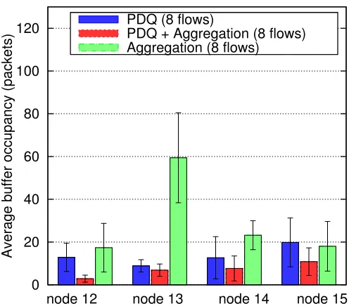
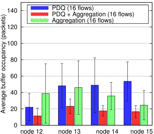
We used different types of topologies for simulation. They are the grid topology in figure 6.1 consisting of 49 nodes, cluster topology shown in figure 6.2 consisting of 36 nodes and random topologies shown in figures 6.3 and 6.4 consisting of 25 and 16 nodes respectively. For each topology we experiment with different number of flows (4, 8, 12 and 16) and observe the aggregate throughput, network utility, fairness index, average network delay and the average buffer occupancy at intermediate nodes with both the schemes: with and without aggregation. We also record the aggregation opportunities for the first two topologies to quantify the benefit of aggregation.

(51)

to lie somewhere between 50 to 60 percent. Figures 6.20 and 6.21 show the results. Under low medium utilization, the nodes will have comparatively less aggregation opportunities, but still it is observed that PDQ+Aggregation schemes gives better aggregation throughputs while preserving the fairness index.

Figure 6.18 compares the aggregate throughputs from theoretical expressions of equations 3.9 and 3.10 and the simulated ones. From the graph, we can see that the theoretical expressions overestimate the actual simulated results. Also, the degree of overestimate increases with the number of flows. One of the possibilities of this overestimation is due to the fact that we do not take into account the overheads caused by the UW header and the aggregation header in theoretical calculations. The other possibility is that we do not consider the degradation due to retransmissions.

In another set of experiments, we study the behaviour of the aggregation scheme with respect to different channel rates. We experiment four flows on random topology of figure 6.4. The flows are from nodes 2 to 0, 8 to 3, 9 to 4 and 13 to 5. The channel rates used are 11b (1, 2, 5.5 and 11Mbps) and 11g(54Mbps). The packet size of the application is 50 bytes. For each of these channel rates, we study aggregate throughput, network utility and fairness index for the aforementioned setting. For these experiments, it is observed that as raw the channel rate increases, the aggregate throughput (figure 6.48) also increases. For an application packet size of 50 bytes, the aggregate throughput steadily increases from about 60 percent for 1Mbps to about 100 percent for 54Mbps. The aggregate network utility for each of the channel rates increases is at least slightly better as shown in figure 6.49a. However, the fairness index for almost every channel rate is worse than the scheme without aggregation(figure 6.49b). Thus, even though aggregation increases the aggregate throughput considerably and network utility by a small amount, this is at the cost of a lower fairness index.

We also study how aggregation performs on real traffic scenarios of the internet.To emulate this, we generate traffic of packet sizes 40, 60, 80, 100, 200, 576 and 1400 bytes randomly with weights 40, 15, 10, 5, 5, 5 and 20 percent respectively. We simulate these traffic patterns with 4, 8, 12 and 16 flows on the grid topology. The results are shown from figures 6.37 through 6.42.

6.2.1 Parameters

(52)

Figure 6.1: Grid topology (49 nodes)

(53)

Figure 6.3: Random topology 1 (25 nodes)

(54)

Table 6.1: OPNET simulation parameters

Parameter value

Transmit power 0.001W

Packet Reception power threshold -67

Routing protocol AODV

Channel rate 11Mbps

RTS threshold None

Application demand type Exponential

Average demand rate 30000000 packets/hour

Transport protocol UDP

Aggregation threshold 1400 bytes

(55)

0 20000 40000 60000 80000 100000 120000 140000

Aggregate Throughput (Bps)

4 flows 8 flows 12 flows 16 flows PDQ

PDQ + Aggregation Aggregation

Figure 6.5: Aggregate Throughput (Random topology 1, 11 Mbps channel rate, exponential distribution)

0 10000 20000 30000 40000 50000 60000

(56)

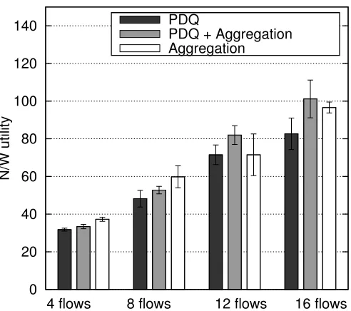
0 20 40 60 80 100 120 140

N/W utility

Figure 6.7: Network utility (Random topology 1, 11 Mbps channel rate, exponential distribu-tion)

0 20 40 60 80 100 120

N/W utility

(57)

0 0.2 0.4 0.6 0.8 1 1.2

Fairness Index

Figure 6.9: Fairness Index (Random topology 1, 11 Mbps channel rate, exponential distribution)

0 0.2 0.4 0.6 0.8 1 1.2

Fairness Index

(58)

0 5 10 15 20 25 30

Average buffer occupancy (packets)

node 12 node 13 node 14 node 15 PDQ (4 flows)

PDQ + Aggregation (4 flows) Aggregation (4 flows)

Figure 6.11: Average buffer occupancy (Random topology 1, 11Mbps channel rate, 4 flows, exponential distribution)

0 20 40 60 80 100 120

(59)

0 20 40 60 80 100 120 140 160

Figure 6.13: Average buffer occupancy (Random topology 1, 11Mbps channel rate, 12 flows, exponential distribution)

0 20 40 60 80 100 120 140

(60)

0 20 40 60 80 100 120

Figure 6.15: Average buffer occupancy (Random topology 1, 1 Mbps channel rate, 8 flows, exponential distribution)

0 20 40 60 80 100 120 140 160

(61)

0 20 40 60 80 100 120 140

Figure 6.17: Average buffer occupancy (Random topology 1, 1 Mbps channel rate, 16 flows, exponential distribution)

0 20000 40000 60000 80000 100000

4 flows 8 flows 12 flows 16 flows PDQ (simulated)

PDQ+Aggregation (simulated) PDQ (theory)

PDQ+Aggregation (theory)

(62)

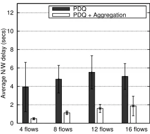
0 2 4 6 8 10 12

Average N/W delay (secs)

PDQ + Aggregation

Figure 6.19: Average network delay (Random topology 1, 11 Mbps channel rate, exponential distribution) 0 10000 20000 30000 40000 50000 60000 70000 80000

(a) Aggregate throughput

0 20 40 60 80 100 120 140 N/W utility

(b) Network Utility

0 0.2 0.4 0.6 0.8 1 1.2 Fairness Index

(c) Fairness Index

Figure 6.20: Random topology 1, 11 Mbps channel rate, exponential distribution, 50-60 percent medium utilization 0 5000 10000 15000 20000 25000 30000

(a) Aggregate throughput

0 20 40 60 80 100 120 140 N/W utility

(b) Network Utility

0 0.2 0.4 0.6 0.8 1 1.2 Fairness Index

(c) Fairness Index

(63)

0 20000 40000 60000 80000 100000 120000 140000

Figure 6.22: Aggregate throughput (Cluster topology, 11 Mbps channel rate, exponential dis-tribution)

0 20 40 60 80 100 120 140

N/W utility

(64)

0 0.2 0.4 0.6 0.8 1 1.2

Fairness Index

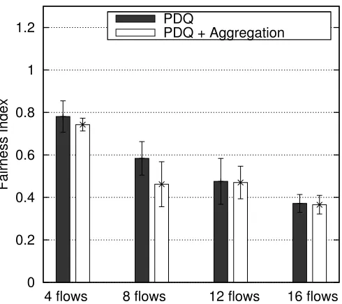
Figure 6.24: Fairness index (Cluster topology, 11 Mbps channel rate, exponential distribution)

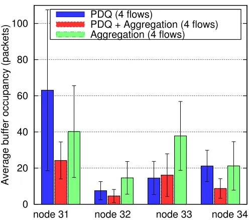
0 20 40 60 80 100

(65)

0 20 40 60 80 100 120

Figure 6.26: Average buffer occupancy (Cluster topology, 11 Mbps channel rate, 8 flows, expo-nential distribution)

0 20 40 60 80 100 120 140 160

(66)

0 20 40 60 80 100 120 140

Figure 6.28: Average buffer occupancy (Cluster topology, 11 Mbps channel rate, 16 flows, exponential distribution)

0 20000 40000 60000 80000 100000 120000 140000

Aggregation Opportunities

4 flows 8 flows 12 flows 16 flows

(67)

0 2 4 6 8 10 12 14

PDQ + Aggregation

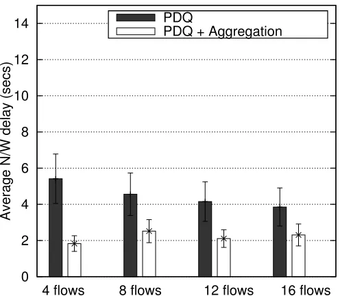
Figure 6.30: Average network delay (Cluster topology, 11 Mbps channel rate, exponential distribution)

0 20000 40000 60000 80000 100000

PDQ + Aggregation

(68)

0 20 40 60 80 100 120 140

N/W utility

PDQ + Aggregation

Figure 6.32: Network utility (Grid topology, 11 Mbps channel rate, exponential distribution)

0 0.2 0.4 0.6 0.8 1 1.2

Fairness Index

PDQ + Aggregation

(69)

0 2 4 6 8 10 12 14

PDQ + Aggregation

Figure 6.34: Average network delay (Grid topology, 11 Mbps channel rate, exponential distri-bution)

0 10 20 30 40 50 60 70

Average Buffer Occupancy (packets)

4 flows 8 flows 12 flows 16 flows node 16(PDQ)

node 16(PDQ+Aggregation) node 18(PDQ)

node 32(PDQ+Aggregation)

(70)

0 50000 100000 150000 200000

Figure 6.36: Aggregation opportunities (Grid topology, 11 Mbps channel rate, exponential distribution)

0 20000 40000 60000 80000 100000

PDQ + Aggregation

(71)

0 20 40 60 80 100 120 140

N/W utility

PDQ + Aggregation

Figure 6.38: Network utility (Grid topology, 11 Mbps channel rate, exponential distribution, internet packet sizes)

0 0.2 0.4 0.6 0.8 1 1.2

Fairness Index

PDQ + Aggregation

(72)

0 2 4 6 8 10 12 14

PDQ + Aggregation

Figure 6.40: Average network delay (Grid topology, 11 Mbps channel rate, exponential distri-bution, internet packet sizes)

0 10 20 30 40 50

4 flows 8 flows 12 flows 16 flows node 16(PDQ)

node 32(PDQ+Aggregation)

(73)

0 50000 100000 150000 200000

Figure 6.42: Aggregation opportunities (Grid topology, 11 Mbps channel rate, exponential distribution, internet packet sizes)

0 10000 20000 30000 40000 50000 60000 70000

PDQ + Aggregation

(74)

0 20 40 60 80 100 120

N/W utility

PDQ + Aggregation

Figure 6.44: Network utility (Random topology 2, 11 Mbps channel rate, exponential distribu-tion)

0 0.2 0.4 0.6 0.8 1 1.2

Fairness Index

PDQ + Aggregation

(75)

0 20 40 60 80 100 120 140 160 180

4 flows 8 flows 12 flows 16 flows node 1(PDQ) node 1(PDQ+Aggregation) node 6(PDQ) node 6(PDQ+Aggregation) node 11(PDQ) node 11(PDQ+Aggregation) node 12(PDQ) node 12(PDQ+Aggregation)

Figure 6.46: Average buffer occupancy per node (Random topology 2, 11 Mbps channel rate, exponential distribution) 0 2 4 6 8 10 12 14 16 18

PDQ + Aggregation

(76)

0 10000 20000 30000 40000 50000 60000 70000 80000 90000

1 Mbps 2 Mbps 5.5 Mbps 11 Mbps 54 Mbps PDQ

PDQ + Aggregation

Figure 6.48: Aggregate throughputs (Random topology 2, 4 flows, Different channel rates)

0 10 20 30 40 50 60 70 80 N/W utility

PDQ + Aggregation

(a) Network Utility

0 0.2 0.4 0.6 0.8 1 1.2 Fairness Index

PDQ + Aggregation

(b) Fairness Index

(77)

Figure 6.50: 4 node Linux testbed topology

0 100 200 300 400 500 600 700 800

Aggregate throughput (Kbps)

50 bytes 100 bytes 200 bytes PDQ

PDQ + Aggregation

Figure 6.51: Aggregate throughput, Linux testbed, 11 Mbps channel rate

6.3 Linux testbed results

(78)

Chapter 7

Summary and future work

In this thesis, we presented a scheme of packet aggregation based backpressure scheduling in wireless multihop networks. Our goal was to incorporate the tool of packet aggregation in the backpressure based scheduling technique and to gain throughput benefits without sacrificing the fairness index of the network. We simulated our scheme in OPNET and also implemented it on a testbed running Linux kernel. Our results show that our scheme of packet aggregation based backpressure scheduling achieves better aggregate throughput that just the backpressure based scheduling scheme without causing a degradation in the fairness index. Also the other important factors like average network delay and congestion at intermediate nodes are improved with the help of our aggregation scheme. We studied our scheme on different topologies.

We do not explicitly consider the effects of noise in the background. The effects of noise could be detrimental to the aggregation scheme. This is because, the presence of noise increases the bit error probability and hence the probability of packet errors increases with the size of the packet. Thus in that case, a threshold needs to be determined which balances the benefits and drawbacks of aggregation by choosing a proper packet size. This is one of the directions.

(79)

REFERENCES

[1] http://www.opnet.com. [2] http://www.netfilter.org/. [3] http://madwifi-project.org/. [4] http://hop.cs.umass.edu/.

[5] Ian F. Akyildiz, Xudong Wang, and Weilin Wang. Wireless mesh networks: a survey. Computer Networks, 47(4):445 – 487, 2005.

[6] U. Akyol, M. Andrews, P. Gupta, J. Hobby, I. Saniee, and A. Stolyar. Joint scheduling and congestion control in mobile ad-hoc networks. pages 619 –627, april 2008.

[7] R. Bruno, M. Conti, and E. Gregori. Mesh networks: commodity multihop ad hoc networks. Communications Magazine, IEEE, 43(3):123 – 131, march 2005.

[8] Dah-Ming Chiu and Raj Jain. Analysis of the increase and decrease algorithms for con-gestion avoidance in computer networks. Computer Networks and ISDN Systems, 17(1):1 – 14, 1989.

[9] E. Fasolo, M. Rossi, J. Widmer, and M. Zorzi. In-network aggregation techniques for wire-less sensor networks: a survey. Wireless Communications, IEEE [see also IEEE Personal Communications], 14(2):70–87, 2007.

[10] Laura Galluccio, Andrew T. Campbell, and Sergio Palazzo. Concert: aggregation-based congestion control for sensor networks. InSenSys ’05: Proceedings of the 3rd international conference on Embedded networked sensor systems, pages 274–275, New York, NY, USA, 2005. ACM.

[11] S. Ganguly, V. Navda, Kyungtae Kim, A. Kashyap, D. Niculescu, R. Izmailov, Sangjin Hong, and S.R. Das. Performance optimizations for deploying voip services in mesh net-works. Selected Areas in Communications, IEEE Journal on, 24(11):2147 –2158, nov. 2006.

[12] Thomas F. Herbert and Thomas F. Herbert. Linux TCPIP networking for embedded systems. Charles River Media, 2007.

[13] A.P. Iyer, G. Deshpande, E. Rozner, A. Bhartia, and Lili Qiu. Fast resilient jumbo frames in wireless lans. pages 1 –9, july 2009.