Performance Tuning of MapReduce Programs.

(1)

ABSTRACT

K.C., KAMAL. Performance Tuning of MapReduce Programs. (Under the direction of Dr. Vincent W. Freeh.)

This dissertation addresses performance tuning of MapReduce programs. The MapReduce framework simplifies processing of large datasets across a large number of machines as a user only needs to implementmapand reducefunctions to create a scalable distributed application. The framework takes care of all other operations such as creating tasks for each function, parallelizing the tasks, distributing data, and handling machine failures. MapReduce programs run in both Hadoop and YARN. Hadoop is a computing framework built on the design of the original MapReduce framework and YARN is a generalized container oriented large scale data processing framework that runs MapReduce applications.

In this dissertation, we first characterize MapReduce programs based on CPU and IO usage of a map task. Our findings show that, based on the similarity of performance of applications under different task parallelism setting, MapReduce applications can be grouped into three categories – IO-intensive, Balanced, and CPU-intensive using cutoffs for the CPU usage. Ap-plications belonging to each group exhibit similar map completion time characteristics.

Second, we develop a static tuning method for setting task parallelism for MapReduce programs. We evaluate thirteen MapReduce applications from all three application categories. We used two clusters with different architecture and obtained the same finding thatIO-intensive applications have best normalized map task parallelism of below 1, Balanced have normalized map task parallelism of 1 or above, and CPU-intensive have normalized map task parallelism close to 1. Normalized map task parallelism is the ratio of the number of map tasks with respect to the number of CPU contexts present in a system. This static method of using task parallelism values based on the category of an application is more efficient than exhaustively profiling or using a default setting.

(2)

Fourth, we study the performance effects of data scaling and configuration parameters on MapReduce programs when running in a large cluster having 540 nodes. We find that IO intensive applications do not scale when data size increases. Configuration parameters that change task parallelism and overlap affect application performance. This study also uncovers issues that occur at large scale such as production of huge logs, need for changing allocation strategy for tasks that coordinate application execution, and need for using data types that can handle calculations involving large numbers without causing overflows.

(3)

(4)

Performance Tuning of MapReduce Programs

by Kamal K.C.

A dissertation submitted to the Graduate Faculty of North Carolina State University

in partial fulfillment of the requirements for the Degree of

Doctor of Philosophy

Computer Science

Raleigh, North Carolina

2015

APPROVED BY:

Dr. William Enck Dr. David Thuente

Dr. Gregory T. Byrd Dr. Vincent W. Freeh

(5)

DEDICATION

(6)

BIOGRAPHY

(7)

ACKNOWLEDGEMENTS

I want to thank my advisor Prof. Vincent W. Freeh for his guidance, advice, and feedback throughout my PhD. He has taught me how to conduct research, how to set research goals, and how to accomplish them. He was always there to show me way whenever I faced any problem. Working with him during paper submissions and presentations was always a motivating expe-rience. I will always fondly look upon my experience working with him as a PhD student. I am very thankful to him for having been the main part of this PhD journey.

(8)

TABLE OF CONTENTS

LIST OF TABLES . . . vii

LIST OF FIGURES . . . ix

Chapter 1 Introduction . . . 1

1.1 Thesis statement . . . 5

1.2 Contributions . . . 6

1.3 Dissertation outline . . . 7

Chapter 2 Related work . . . 8

2.1 Hadoop and YARN architecture . . . 8

2.1.1 YARN . . . 10

2.1.2 Map task phases . . . 10

2.1.3 Hadoop applications . . . 11

2.2 Hadoop tuning . . . 12

2.3 Feedback based control . . . 13

2.4 MapReduce in a large cluster . . . 13

2.5 Resource allocation . . . 14

2.6 Selecting optimized techniques . . . 14

2.7 Log compression . . . 15

2.8 Workload analysis . . . 15

2.9 Hadoop schedulers . . . 16

Chapter 3 MapReduce application profiling . . . 17

3.1 Cluster description . . . 17

3.2 Measurements . . . 18

3.3 Performance analysis . . . 18

3.4 Chapter summary . . . 21

Chapter 4 MapReduce characterization and static tuning . . . 22

4.1 Approach . . . 22

4.1.1 Hadoop counters . . . 23

4.1.2 CPU utilization spectrum . . . 24

4.2 Predicting best MSVs . . . 25

4.2.1 CPU and IO behavior . . . 28

4.3 Performance analysis . . . 29

Chapter 5 Dynamic tuning . . . 33

5.1 Resource usage monitoring . . . 34

5.2 Feedback controllers . . . 39

5.3 Dynamic tuning in Hadoop . . . 39

(9)

5.3.2 Exceptions . . . 41

5.3.3 Implementation . . . 42

5.3.4 Hadoop applications and datasets . . . 42

5.3.5 Performance analysis . . . 43

5.3.6 System behavior for dynamic and static MSVs . . . 46

5.4 Dynamic tuning in YARN . . . 51

5.4.1 Controllers . . . 51

5.4.2 Implementation . . . 54

5.4.3 Evaluation . . . 54

5.4.4 Performance comparison . . . 55

5.4.5 Resource usage . . . 57

5.4.6 Tuning CCS for multiple workloads . . . 60

Chapter 6 MapReduce in a large cluster . . . 62

6.1 Parallelism and overlap configuration . . . 63

6.2 Experimental methodology . . . 64

6.3 Data size scaling . . . 65

6.3.1 Scaling results . . . 67

6.3.2 Resource usage analysis . . . 68

6.4 Parallelism and overlap . . . 70

6.5 Experiences on the large cluster . . . 72

6.5.1 Application master sizing . . . 73

6.5.2 Log aggregation . . . 73

6.5.3 Failures in large clusters . . . 74

Chapter 7 Log compression. . . 76

7.1 Background . . . 77

7.2 Design . . . 78

7.3 Online compression . . . 80

7.3.1 Evaluation . . . 80

7.4 Offline compression . . . 81

7.5 Loggrep . . . 82

Chapter 8 Concluding remarks . . . 84

(10)

LIST OF TABLES

Table 3.1 Normalized performance and the best completion time (in parentheses) for different MSVs on cluster P6 with 150GB data size. . . 19 Table 3.2 Normalized performance the best completion time (in parentheses) for

dif-ferent MSVs on cluster P6 with 300GB data size. . . 19 Table 3.3 Normalized performance the best completion time (in parentheses) for

dif-ferent MSVs on cluster I6 with 150GB data size. . . 20 Table 3.4 Normalized performance and the best completion time (in parentheses) on

cluster P10 with 500GB data size. . . 20

Table 4.1 Utilization and throughput in the ascending order of CPU UTIL for P6 cluster. 23 Table 4.2 Normalized performance and the best completion time (in parentheses) for

different MSVs on the cluster P6 with 150GB data size. . . 26 Table 4.3 Normalized performance the best completion time (in parentheses) for

dif-ferent MSVs on cluster P6 with 300GB data size. . . 27 Table 4.4 Normalized performance the best completion time (in parentheses) for

dif-ferent MSVs on cluster I6 with 150GB data size. . . 28 Table 4.5 Aggregate normalized performance values and maximum slowdown

percent-ages (inside parentheses) for the three tested cases. . . 30

Table 5.1 Normalized performance and the best completion time (in parentheses) for static and dynamic MSVs on P10 cluster with 600GB data size. . . 44 Table 5.2 Relative comparative map completion times for various CCS settings. The

best practice column shows total elapsed time in seconds. . . 56

Table 6.1 Three types of applications in PUMA benchmark. . . 63 Table 6.2 Comparative data movement through the MapReduce phases for Small dataset. 64 Table 6.3 Number of reduce tasks for the three data sizes. . . 66 Table 6.4 Completion times (TS, TM, TL) and computation time per unit data for data

sizes. . . 67 Table 6.5 Average resource utilization of a single node in AWB (Datasets: S=small,

M=medium, L=large). . . 68 Table 6.6 Different memory sized AM for medium dataset. The partial failure is an

empirically observed result and was not consistently repeatable. A “P” in the table indicates that at least one time a failure occurred and at least one time a successful completion occurred. . . 73 Table 6.7 Log size (in TB) for the three datasets. . . 74 Table 6.8 Number and percentage of INFO, WARN, and ERROR log messages for

large dataset. . . 74

Table 7.1 Log size (in TB) for the three datasets in the AWB cluster. . . 76 Table 7.2 Comparison of compressed size, time to compress/decompress, and the rate

(11)

Table 7.3 Comparison of compressed and uncompressed log size and total application completion time. The compressed column also shows the size in % compared to the uncompressed size. . . 81 Table 7.4 Comparison of compression for different number of log messages for our

ap-proach,gzip, and bzip2. . . 81 Table 7.5 Compression performance of offline approach. . . 82 Table 7.6 Comparison of search time for fgrep and our approach for the logs shown in

(12)

LIST OF FIGURES

Figure 2.1 Workflow in the Hadoop architecture. . . 9

Figure 2.2 Map task phases. . . 11

Figure 4.1 Relationship between CPU UTIL and IO THRPUT. . . 24

Figure 4.2 Classification for applications running on P6 cluster. . . 29

Figure 4.3 Classification for applications running on I6 cluster. . . 30

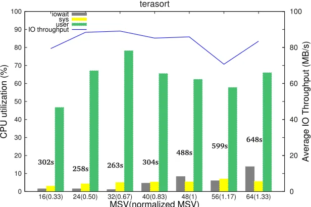
Figure 4.4 CPU utilization, IO throughput, and completion time (shown in relative vertical heights) of an IO-intensiveapplication (terasort). . . 31

Figure 4.5 CPU utilization, IO throughput, and completion time (shown in relative vertical heights) of a Balanced application (invertedindex). . . 31

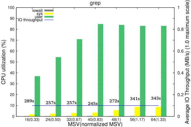
Figure 4.6 CPU utilization, IO throughput, and completion time (shown in relative vertical heights) of a CPU-intensiveapplication (grep). . . 32

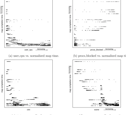
Figure 5.1 Relation of the considered metrics with map completion time. . . 37

Figure 5.2 Relation of the used metrics and the score with map completion time. . . . 38

Figure 5.3 Feedback control for dynamically changing CCS. . . 39

Figure 5.4 Bezier approximation of MSV vs. score for a Hadoop application (ranked-invertedindex). . . 40

Figure 5.5 Map completion progress comparison for rankedinvertedindex for static and dynamic MSVs. . . 45

Figure 5.6 System behavior for dynamic MSV of an IO-intensive region application (rankedinvertedindex). . . 46

Figure 5.7 System behavior for dynamic MSV of a Balanced region application (ter-mvectorperhost). . . 47

Figure 5.8 System behavior for dynamic MSV of a CPU-intensive region application (terasort(L10,D1)). . . 47

Figure 5.9 System behavior of rankedinvertedindex for static MSV 24. . . 49

Figure 5.10 System behavior of rankedinvertedindex for static MSV 48. . . 49

Figure 5.11 Characteristics of rankedinvertedindexterasort(L200,D100) for dynamic MSV. 50 Figure 5.12 Bezier approximation of score against CCS (rankedinvertedindex). . . 53

Figure 5.13 CCS changing for terasort for all tuning approaches. . . 56

Figure 5.14 Resource usage of anodemanager during map execution of terasortfor de-fault CCS. . . 57

Figure 5.15 Resource usage of a nodemanagerduring map execution ofterasortfor best practices CCS. . . 58

Figure 5.16 Resource usage of a nodemanagerduring map execution of an IO-intensive application (terasort) for PD. . . 58

Figure 5.17 Resource usage of anodemanager during map execution of a Balanced ap-plication (invertedindex) for PD. . . 59

Figure 5.18 Resource usage of anodemanagerduring map execution of a CPU-intensive application (grep) for PD. . . 59

(13)

Figure 6.1 Network usage of IO-intensiveapplication terasort. . . 69 Figure 6.2 Best performing combinations of CCS and SS for all six applications. . . 71

(14)

Chapter 1

Introduction

Processing large multi terabyte datasets is unsuitable on a single machine due to its limited resource capabilities for processing and storage. Examples of large unstructured datasets are collections of crawled web documents, user web requests, or system logs. Processing them in timely manner requires processing capability equivalent to hundreds or thousands of machines. Using a large number of machines requires addressing issues related to parallel computation, data distribution, input/output data storage, and failure handling. Taking this in consideration, Dean et al. developed a generic data processing framework called MapReduce, which consists of a programming abstraction as well as a runtime framework that distributes computation across several machines, distributes input and processed data, and handles failures [42]. All MapReduce programs are expressed as map and reduce functions. A map function processes each individual input data record and produces intermediate data in key-value format. Areduce function processes the intermediate data in groups of key-value pairs with same keys. A large number of data processing applications can be expressed as MapReduce programs [5, 12, 31, 34, 37]. This illustrates the importance of MapReduce framework.

(15)

determine how these operations are performed. For example, some of the parameters determine the task distribution across the machines whereas some influence the intermediate operation, such as map output buffer sizes, enabling compression of intermediate data. Using appropriate configuration values can help an application to complete faster, whereas misconfiguration can slow down an application.

Several of Hadoop’s resource management limitations were addressed in a computing frame-work called YARN. YARN improves the original MapReduce [42] architecture by separating resource management from computing framework [75]. Instead of Hadoop, where tasks are cre-ated only for map and reduce functions, YARN pushes forward the concept of general process abstractions called containers that not only run map and reduce tasks but also run other user submitted programs. The generalization of resource management makes it easier to deploy not only MapReduce applications, but also other large scale data processing applications such as Spark [82] and Tez [4, 75].

Previous research has shown that the performance of MapReduce applications changes in Hadoop and YARN depending upon the values of configuration parameters [48, 53, 59]. Perfor-mance tuning of these configuration parameters (more than 150) is combinatorially intractable. The most common method for selecting best configuration values is trying several possible val-ues and manually tweaking them until a MapReduce application completes in the least amount of time [6]. This process quickly becomes tedious and inefficient when finding best values for more than one MapReduce application. It is not feasible to exhaustively determine the best configuration. For example, in our work, it took one week to find the best configuration param-eter values for eighteen applications and we only tested a handful of configuration paramparam-eters. Due to such long time required to profile applications for all possible values, this method is mostly impractical in Hadoop deployments. Thus, it is desirable to have a mechanism to select configuration parameters that improve performance of an application.

(16)

Application characterization and static tuning

Map slot value (MSV) is the maximum number of map tasks that run concurrently on a Hadoop compute node. Its misconfiguration can create significant performance degradation. Our re-search shows that a Hadoop application has a narrow range of MSVs for which its performance is the best. Furthermore, there is not a single MSV that has the best performance for all Hadoop applications. For example, in one of our experimental clusters there are four MSVs that have the best performance for at least one application, but these MSVs have maximum performance degradation as high as 132%. Thus, it is important to know the best MSV for an application in order to avoid its performance degradation. In this dissertation, we present a method to reliably predict the best MSV with low-overhead. Our method uses two new Hadoop counters that measure per-map task CPU utilization and IO throughput.

Dynamic tuning

In Hadoop/YARN, performance tuning is largely manual and is done via configuration parame-ters. The configuration parameters control the allocation of tasks, intermediate buffer sizes, data compression, and other large number of internal operations. Achieving better system resource utilization therefore requires carefully tuning the configuration parameters, which are around 150 in number [22]. Previous work shows between 1.5 and 4 times slowdown of MapReduce ap-plications due to misconfiguration [56, 53, 48]. In this dissertation, we investigate and develop dynamic tuning approach for Hadoop/YARN in order to improve its resource allocation as well as performance of MapReduce applications during the runtime. Our tuning approach focuses on the Hadoop parameter called map slot value and YARN value called concurrent container slot.

(17)

applications, and automatically tunes the configuration parameters. In this dissertation, we develop and evaluate dynamic tuning methods to achieve these goals.

Our dynamic tuning method changes MSV/CCS during runtime of a MapReduce applica-tion. It is based on using a feedback controller. We design and evaluate a feedback controller for Hadoop and three different types of feedback controllers for YARN. During the execution of an application, the feedback controller changes MSV/CCS in response to the change in monitored resource usage of a system. For YARN, we implement a container suspend mechanism that allows to monitor system resource usage at shorter intervals. When CCS is lowered, the extra containers are suspended, which reduces total number of IO requests or CPU contention. This helps to immediately get rid of bottlenecks. The efficient resource usage due to the feedback controller ensures faster completion time for applications.

There are two advantages to dynamically controlling MSV/CCS over static tuning. First, it does not require any application profiling prior to running the application. Second, it can respond to changes in best MSV/CCS during the execution of an application. Our findings show that our dynamic tuning method for MSV/CCS achieves more efficient resource usage. For Hadoop, the dynamic tuning performs within 4.6% of the static, profile-determined best MSV with cold start and improves by as much as 5% with warm start. For YARN, the performance improvement is as much as 28% and 60% respectively when compared to the best practice and the default settings.

Running MapReduce applications in a large cluster

Large cluster study provides a reference to assess performance behavior of MapReduce appli-cations. We perform three types of evaluation of MapReduce applications in a 540-node large cluster called AWB [24]. Our first evaluation explores data scaling behavior of six MapReduce applications that have wide variety in map and reduce task characteristics. Our second eval-uation explores the effect of configuration parameters on application performance. Previous studies on small clusters (10 and 14 nodes) have shown that tuning task parallelism improves overall performance [48, 53, 56]. However, the effects of changing parallelism and overlap of tasks in MapReduce applications in a larger cluster have not been studied before. Our third evaluation discusses experiences of running applications in a large cluster. This includes findings that are not noticeable in smaller clusters.

(18)

configuration values are dependent upon application CPU and IO characteristics. Our findings on AWB also shows observations that are not noticeable in a smaller cluster. We discuss three such observations in this dissertation — appropriately sizing a component of an application, suitability of the type of information level for huge application logs produced by MapReduce applications, and errors that occur when processing large datasets.

Log compression

Hadoop/YARN applications generate large amount of logs which can impose overhead of storing them in local disks as well as the Hadoop Distributed Filesystem (HDFS). To eliminate this storage overhead as well as to minimize compute overhead while doing so, we develop an online log compression scheme that uses the log message formats to write only log identifier in the log message. For this we intercept the log message before it is handed over to the logging layer of Hadoop/YARN and write the compressed output to the disk. Our findings show that the storage space of logs is reduced to one-third of the raw uncompressed log file while incurring only 3% overhead on the application completion time.

1.1 Thesis statement

The focus of this dissertation is to research performance tuning techniques for MapReduce pro-grams. To achieve this, we assess performance behavior of MapReduce applications in a large cluster, characterize MapReduce applications, research static and dynamic tuning methods, and develop compression technique to minimize log storage overhead. Our findings show that MapReduce application performance is affected by application characteristics and configuration parameters. The large cluster study sheds light on application scaling behavior, effect of con-figuration parameters, and experiences that divulge issues occurring at large scale. Application characterization shows that applications can be grouped into three categories based on their CPU and IO characteristics. These categories describe their performance behavior. Using the application characterization information, static tuning technique can be developed that would provide a configuration value for each category of applications. Dynamic tuning techniques achieve better resource utilization and faster application completion times without the need for prior application profiling. Online log compression achieves savings in log storage space without significantly affecting application completion time.

The findings of this dissertation therefore support the following thesis statement.

MapReduce application performance is dependent upon its CPU and IO

(19)

application task profile to perform coarse grained tuning where the task parallelism

is set before the application runs. Dynamic tuning does not use any prior application profile and instead uses instantaneous resource usage of the system during runtime

to perform fine grained tuning.

1.2 Contributions

In this dissertation, we make the following contributions.

We perform extensive profiling to study the performance effect of a Hadoop configura-tion parameter.We run several MapReduce applications for different values of a Hadoop parameter determining parallelism of map tasks and investigate the difference in per-formance. This study shows that the performance improves with appropriate setting of the parameter whereas the performance degrades with inappropriate setting. This study motivates our research on performance tuning. It further provides basis for application classification that helps in tuning.

We develop a static tuning method that uses CPU and IO resource usage values of an application’s map task. Our static tuning method groups an application into one of the three regions by using the value of a per-map task CPU utilization counter. These regions are created by correlating the per-map task counter value and map completion time from the extensive profile of the application completion times. The profile of the application completion times are of MapReduce applications that encompass the entire spectrum of the per-map task CPU counter value. Each region is then mapped to a range of best MSVs. An application can use an MSV from its region’s range of best MSVs. This approach overcomes the disadvantage of extensive profiling and performs better in comparison to arbitrarily selecting an MSV.

We identify metrics that can relate to the performance of an application during runtime. Operating system maintains many system metrics that track utilizations of CPU, mem-ory, disks, software queues, context switches, and other resources. A key part of our work involves identifying metrics that correlate with the performance of a MapReduce applica-tion. This enables us to know whether the metric measurements for a parallelism setting cause performance improvement or degradation. We analyze several available system met-rics and find three metmet-rics, which when combined together correlate with the performance of an application.

(20)

more fine grained best parallelism selection. To overcome these drawbacks, we develop a dynamic tuning approach that uses the metrics correlated with an application’s per-formance. Our approach uses feedback controllers that dynamically change MapReduce parallelism by using the instantaneous values of these metrics. The metrics indicate the degree of resource pressure on the system. If the resource pressure is low, the controller increases parallelism andvice-versa. This dynamic approach tunes MapReduce task par-allelism to achieve best or nearly best performance.

We perform study of MapReduce application performance in a large cluster. We run a variety of MapReduce applications on a 540-node cluster to study the data scaling behav-ior, effects of configuration parameters for parallelism and overlap, and issues occurring on a large MapReduce cluster. Findings of this study show that in a large cluster there exist differences among applications on data scaling behavior and configuration parameter tuning plays an important role in improving application performance. This study further validates the importance of studying behavior of MapReduce applications that have wide variety in CPU and IO characteristics.

We develop a low overhead online compression technique to reduce log storage space. MapReduce logs occupy large storage space. To reduce the storage space overhead, we develop an online log compression technique that encodes the log message before it is written to the disk. This saves valuable local storage space as well as space in distributed file system.

1.3 Dissertation outline

(21)

Chapter 2

Related work

In this chapter, we provide background on Hadoop/YARN and describe related work in our research area. The categories of related work discussed are based on the types of problem addressed in characterization and performance tuning of MapReduce applications, large cluster study, and log compression. We start with the description of Hadoop/YARN architecture.

2.1 Hadoop and YARN architecture

The original Hadoop, which is implemented based on MapReduce [42], consists of a jobtracker server which coordinates with multiple tasktracker clients [13]. Jobtrackeraccepts MapReduce jobs from users and a typical MapReduce job processes large amounts of data. Jobtrackers and tasktrackers handle the computation part of a Hadoop job. The data storage and retrieval is handled by the Hadoop distributed file system (HDFS). HDFS is implemented based on Distributed File System (DFS) described in MapReduce [42]. HDFS is formed by aggregating storage of each client node. HDFS is managed by a namenode server, which coordinates with multiple datanode clients. The datanodes are responsible for data storage and run along with tasktrackers in the client nodes. HDFS stores data in large data block sizes such as 64MB or higher [15, 1].

(22)

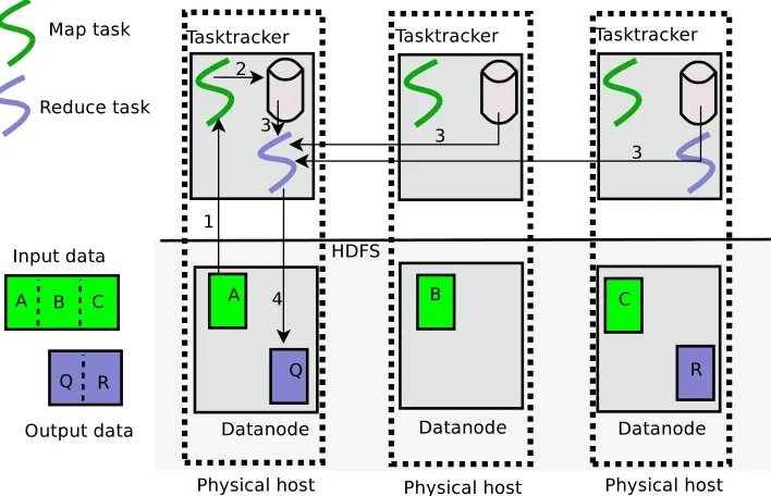
Figure 2.1: Workflow in the Hadoop architecture.

Step 1:After an application is accepted by thejobtracker, it creates a map task for each block of input data. It then assigns the map tasks totasktrackers. The maximum number of tasks that can be assigned is determined by the MSV setting of thetasktracker. A map task processes a block of data and produces key-value output pairs. In the Figure 2.1, a map task is created for each block of input data – A, B, and C.

Step 2:The map task partitions the output according to the range of the key. The number of output partitions equals the number of reduce tasks. The output is then stored in the local disk of the tasktrackernode that runs the map task.

Step 3: A reduce task processes one specific partition of map output. The jobtracker assigns reduce tasks based on the reduce slot values. When the reduce task is processing the data, it copies data from all tasktracker nodes to fetch its assigned partition. This is shown as arrows in Figure 2.1 for reduce task that produces output block “Q” (To reduce the clutter, the arrows for the reduce task in the right-hand node that produces output block “R” are not shown).

Step 4:After reduce task processes the map output key-value pair, it writes the output to HDFS. In the Figure 2.1, the output written to HDFS are the data blocks Q and R.

(23)

applications used in our work, which represent common Hadoop applications, have an average map time of 67% of the total job runtime. The lowest map time for an application is 42% of the total job runtime whereas the highest map time is 85% of the total job runtime. For this reason, we focus on optimizing the map runtime.

2.1.1 YARN

YARN [2, 75] rearchitects the original MapReduce [42] by putting resource management and MapReduce framework in separate modules. This enables YARN to perform only resource management tasks and makes it useful to run other frameworks in addition to MapReduce. YARN consists of a resourcemanager and multiple nodemanagers. Applications run in YARN as containers, which are process abstractions that can run any user program. These containers run in nodemanagers and are allocated by the resourcemanager. Each nodemanager updates its memory and virtual core limits to the resourcemanager [18, 19]. The memory and virtual core request of an application container is then used to determine how many containers the resourcemanagercan allocate to a nodemanager.

When a MapReduce application is deployed, it creates an application master (AM) that runs in a container. The AM asks the resourcemanagerfor containers to run map and reduce tasks. After theresourcemanagerassigns containers to nodes, the application master coordinates their execution in conjunction with nodemanagers. After negotiation of containers, the execution of the MapReduce YARN framework is similar to the original Hadoop framework. A map task processes a block of HDFS data. The map task is typically assigned to a container local to the node that has the input data block. The input to a map task is in the form of key-value pairs. The map task partitions its output by keys. The total number of partitions is equal to the number of reduce tasks. The output is then stored in the local disk. A reduce task processes one specific partition of the map output. The data processed by a reduce task is the aggregated collection of its assigned partition that is copied from the outputs of all map tasks. Reduce tasks write their output, which is the final output, to HDFS. Containers are freed after they complete map or reduce operations.

2.1.2 Map task phases

(24)

Figure 2.2: Map task phases.

the spilling occurs. When the map output buffer is full, the map task empties the buffer by spilling its content to a spill file in the local disk. This is the spill phase. The combine phase is optional and when present, the map task performs a local reduce operation on the map output key-value pairs. In themerge spill phase, the spill files are merged together to produce a single map output file.

Each phase in the map task is either CPU or IO intensive. The CPU intensive phases are compute, collect, sort, and combine. The IO intensive phases are spill and merge spills.

2.1.3 Hadoop applications

In this dissertation, the main applications we use are taken from the Hadoop distribution [11] and PUMA benchmark [33]. PUMA is a Hadoop benchmarking suite developed by Purdue University. PUMA includes three MapReduce programs from the official Hadoop distribution and ten other MapReduce programs. The collection of diverse applications makes it a useful benchmarking suite. In our work, we use six PUMA MapReduce applications together with modified versions ofterasort. The six applications are grep,wordcount,invertedindex, rankedin-vertedindex,terasort, andtermvectorperhost. These are some of the commonly used applications suitable for MapReduce processing [5]. The operations performed by each application are pre-sented below.

grep. This application matches the search pattern in text documents. Its map task searches for a pattern in a file and produces an intermediate tuple <text,1> for each matched text. Reduce task sums the occurrence of the matches and outputs a single tuple <text,n>for each unique matched text, where nis the number of matches.

(25)

invertedindex. This application creates an inverted index, which maps the words to its documents. This index is used by search engines to locate documents containing text words. An example is the index created by Lucene [3]. The map task outputs a tuple <word,document identifier> for each word with the document identifier. Reduce task combines all the matching words in the map output tuples and produces a tuple containing the word and the list of document identifiers.

rankedinvertedindex. This application is similar to invertedindex except that in the mapping between words and documents, the documents are listed in decreasing order of the word appearance frequency. Instead of mapping a single word to the documents, PUMA maps a three word sequence to documents. The three word sequence is generated using another applicationsequence-count. We do not use the sequence-count application and instead use the datasets provided by PUMA, which is the output fromsequence-count.

terasort. This application is frequently used in sort benchmarks [29], where the data consists of 100-byte records with the first ten bytes as the key. Map tasks output the key value pair as it is. The records are partly sorted in the map output buffer and are finally sorted during the shuffle. Before reduce task processes the records, they are already sorted and the reduce task outputs the records as it is in the sorted order.

termvectorperhost. This application determines the most frequently used words present in the documents of a URL [42]. A URL represents the machine host and such information can be useful for search engines. Map task outputs the tuple of URL and termvectors for each document. A termvector is a tuple of a word and its frequency in documents. Reduce task outputs termvectors for each URL in the form of a tuple. Reduce discards the words in the termvectors output, if the frequency of the words do not meet a threshold.

Datasets. We use PUMA datasets in our work [26]. Datasets for grep,wordcount, inverte-dindex, and termvectorperhost are derived from Wikipedia website content. terasort uses the dataset generated by teragen application. teragen is an application present in the Hadoop distribution. rankedinvertedindexuses dataset produced by another PUMA application called multi-wordcount.

2.2 Hadoop tuning

(26)

context switches for different applications. Autotune uses a trained model to tune the number of reduce tasks rather than changing reduce task slots [83].

Starfish uses dynamic instrumentation to profile a Hadoop job and uses this profile to estimate cost of configuration parameters [36, 47, 48, 49]. In contrast, we identify and measure the key metrics with minimal changes to the original system and use the metrics to predict the configuration parameters. Karthik et al. propose RS Maximizer which optimizes Hadoop parameters by matching the resource consumption signature of a job with the ones whose optimal configuration values are already measured experimentally [53]. This technique estimates the Hadoop parameters by using the using performance behavior of existing jobs rather than the using key features to directly obtain the parameter values. MR-online uses tuning rules in conjunction with a hill climbing search to explore configuration parameters in YARN [59].

Our work differs from previous tuning efforts because it does not require prior knowledge, tuning rules, or extensive profiling of applications. Additionally, as our work uses dynamic control, it does not rely on predetermined resource usage threshold.

2.3 Feedback based control

Previous work on feedback based control has been done mostly on dynamically tuning factors affecting system performance and limiting power consumption of a system. Mineric et al. use PI controller to adjust CPU frequency to maintain a set power consumption level [62]. Abdelzaher et al. use PI controller to tune web server’s response quality by using server utilization [32]. This helps to balance server load as the web server can respond with different quality images that have different sizes. Wang et al. use PID controller to adjust the CPU allocations to meet a system response time [77]. Our work utilizes different types of feedback controllers (PID, PD, Waterlevel, and PD+pruning) controllers to tune CCS/MSV using the resource usage metrics.

2.4 MapReduce in a large cluster

(27)

jobs [68]. Another previous work shows that jobs were failing in a large Hadoop cluster due to incorrect configuration of the storage framework [54].

The second related area is scalability. A previous work compares scale-out and scale-up models and investigates the relative effectiveness of scale-up [71]. Similarly, another related work compares the performance of scale-out and scale-up in Hadoop and finds performance improvement with the scale-up model [35]. Another work studies the scalability of an indexing application in Hadoop when changing the cluster size [60]. Another related work uses IO model and data parsing to address performance bottlenecks in Hadoop [52]. Previous work also explores the limitation of Hadoop scalability in terms of its inability to change map and reduce slots for different applications [72].

2.5 Resource allocation

Work in this area mostly focuses on resource sharing across multiple jobs. YARN is the newer resource management framework for Hadoop, which enables an application to specify its re-source requirements [75]. Dominant Rere-source Fairness (DRF) allocates rere-sources on the basis of the dominant resource request of an application [43]. A dominant resource is the one with higher requirement among all the resource types requested by an application. For example, if a user A runs CPU heavy tasks and another user B runs memory heavy tasks, then DRF equalizes CPU share of user A with memory share of user B. After equalizing the resources, the number of tasks to run is computed.

The purpose of these research works is either to ensure fairness across multiple jobs or to differentiate prioritization among multiple jobs. In contrast, our work focuses on maximizing the system resource utilization to achieve faster completion time for a job.

2.6 Selecting optimized techniques

This related work optimizes application performance by selecting best predefined techniques. ATLAS selects alternative implementations in order to optimize the performance of an applica-tion [78]. It uses empirical timings of platform dependent parameters to choose the best method for performing linear algebra operations for that particular hardware. For ATLAS, linear al-gebra operations are limited in number and the timing measurements of all these operations is sufficient for performance optimization. In contrast, a Hadoop application contains different operations inside map function implementations rather than a set of known operations.

(28)

mentioned in the diagnostic rules and does not provide an estimate of the configuration param-eters. These approaches provide an additional method of improving system performance when an application’s usage scenarios can be enumerated before execution or when an application can be reconfigured to use alternative implementations.

2.7 Log compression

There is previous work on log compression [64, 73, 40] and database compression techniques that can be utilized to compress logs [80, 45, 74]. Scalatrace compresses MPI communication traces by preserving time and causality of communication events so as to facilitate deterministic replay and trace extrapolation [64]. The compression scheme shortens the function call traces by identifying repetition of function calls or segment of function calls. Another work uses temporal locality and hashing to separate similar log entries and compresses them [40]. It achieves 30% compression improvement for Apache web server compared togzipof the entire log files. Another work replaces parts of log messages such as date and texts with specific numbers to achieve better compression for applications such as MySQL and syslog [73].

In databases, several column compression techniques have been developed to reduce the data storage requirement. Druid uses dictionary encoding and maps each column page to unique identifier to compress column data [80]. Powerdrill is another database that compresses its column data [45]. C-store uses delta encoding to store only the difference between column data values [74].

2.8 Workload analysis

Work on workload analysis area focuses on creating standardized benchmarks [38]. Mishra et al. categorize the workloads running on Google computer clusters into 3 qualitative categories (small, medium, and large) for each job property such as task duration, CPU, and memory usage [63]. This work does not associate job characteristics with the performance behavior. HiBench provides both micro-benchmark and real-world benchmark for Hadoop [50]. Yahoo Cloud Serving Benchmark (YCSB) is a cloud benchmark that attempts to understand the performance and behavior of cloud data serving systems [41]. TPC-W is a benchmark to test the scalability of e-commerce websites [61].

(29)

2.9 Hadoop schedulers

(30)

Chapter 3

MapReduce application profiling

In this chapter, we describe profiling, which is a common way to find the best map slot value (MSV) for an application. This chapter is based on our work on profiling and static tuning [56]. MSV is a configuration setting in Hadoop that determines the number of concurrent map tasks that can run in a tasktracker node. Profiling involves running an application for all possible MSVs and comparing the map completion time to find the shortest time. The MSV setting for the shortest map completion time is the best MSV.

The advantage of profiling is that it successfully finds the best MSV of an application. However, the disadvantage is that it takes a long time to obtain the map completion time for all MSV settings. For example, in one of our tests of eighteen applications, it took one week to find the best MSV out of 10 MSV choices for every one of the eighteen applications. Due to this reason, it may not be suitable for Hadoop deployments. In the following sections, we describe the clusters used in our dissertation and analyze profiling results for the six Hadoop applications that were introduced in the previous chapter.

3.1 Cluster description

There are three clusters used throughout this dissertation. The best MSV setting obtained during profiling is dependent upon the machine configuration of each cluster. Each cluster’s configuration is described below.

(31)

Cluster P6. This cluster consists of six IBM PowerPC machines. Each node contains two 8-core POWER7 processors with a total of 16 cores and 48 CPU threads, 90GB RAM, and a 10 Gbps Ethernet network link. Hadoop is configured with one jobtracker and five tasktrackers. HDFS is configured with one namenodeand five datanodes.

Cluster P10. This cluster consists of ten IBM PowerPC machines. Each node consists of two 8-core POWER7 processors with a total of 16 cores and 64 CPU threads, 124GB RAM, and a 10 Gbps Ethernet network link. Hadoop is configured with one jobtracker and ninetasktrackers. HDFS is configured with onenamenodeand nine datanodes.

3.2 Measurements

The measurement values shown in this dissertation are median value of three measurements for each MSV/CCS or dynamic setting for each application. Care has been taken to run each set of experiments during the same time period to minimize the effects of background operating system processes. Each measurement value reported in this dissertation has variation within 0.2% for its three measurements.

3.3 Performance analysis

Table 3.1 shows the normalized performance behavior of the fifteen applications for different MSVs for cluster P6 with 150GB data. The best performance value is 1 and it denotes the shortest completion time of an application for the set of MSVs used in the experiments. The normalized MSV is the MSV relative to the number of CPU threads in a node.1 For the PowerPC machine of cluster P6, a normalized MSV of 1 means an actual MSV of 48, which is equal to 1 map task per CPU thread (or 2 map tasks per core). The best MSV is the one for which an application has the shortest completion time. The shortest completion time is shown in parentheses for each application. In cluster P6, MSV is set to values from 16 to 64 with increments of 8. Below 16 and beyond 64, the applications suffer slowdown and those results are omitted.

Table 3.1 shows that there is a best value for each application and there is not a single MSV that is best for all applications. Every application in the table has a unique best MSV. For example, terasort and wordcount have best MSVs of 24 and 56. The last row shows the number of best values for different MSVs. MSVs 24, 40, and 56 are best for 1, 2, and 3 applications. 1_{The machines used in our experiments have hyperthreading enabled due to which the CPU schedulable}

(32)

Table 3.1: Normalized performance and the best completion time (in parentheses) for different MSVs on cluster P6 with 150GB data size.

Data size=150GB, CPU cores per node=24, CPU threads per node=48

Job

MSV(normalized)

16 24 32 40 48 56 64

(0.33) (0.50) (0.67) (0.83) (1) (1.17) (1.33)

terasort 1.17 1(258s) 1.02 1.18 1.89 2.32 2.51

rankedinvertedindex 1.30 1.09 1.01 1(453s) 1.11 1.09 1.23

word count 1.57 1.26 1.26 1.06 1.08 1(564s) 1.04

invertedindex 1.49 1.21 1.21 1.06 1.09 1(620s) 1.02

termvectorperhost 1.38 1.16 1.16 1.02 1.08 1(694s) 1.02

grep 1.18 1.05 1.05 1(245s) 1.11 1.39 1.40

Aggregate 8.09 6.77 6.75 6.32 7.36 7.8 8.22

# of best values 0 1 0 2 0 3 0

Table 3.2: Normalized performance the best completion time (in parentheses) for different MSVs on cluster P6 with 300GB data size.

Job

MSV(normalized)

16 24 32 40 48 56 64

(0.33) (0.50) (0.67) (0.83) (1) (1.17) (1.33)

terasort 1.13 1(519s) 1.06 1.57 2.42 2.49 2.92

word count 1.52 1.22 1.09 1.03 1.03 1(1110s) 1.02

invertedindex 1.49 1.20 1.09 1.03 1.02 1.01 1(1307s)

grep 1.33 1.17 1.05 1(513s) 1.01 1.06 1.03

Aggregate 8.14 6.86 6.42 6.73 7.72 8.03 9.09

One significant MSV is 40, which has lowest aggregate performance value of 6.32. The aggregate value is 6.4% higher than the theoretical best aggregate performance value of 6. But, it has a maximum slowdown of 18% for terasort. Thus, picking MSV 40 for all applications is not a best solution. Additionally, while MSV of 56 is best for the most applications, it has a slowdown of 132% for terasort. This further reinforces that a single MSV is not a best choice for all applications.

(33)

Table 3.3: Normalized performance the best completion time (in parentheses) for different MSVs on cluster I6 with 150GB data size.

Job

MSV(normalized)

4 8 12 16 20 24

(0.25) (0.50) (0.75) (1) (1.25) (1.5)

terasort 1.14 1(2688s) 1.05 1.11 1.34 1.46

rankedinvertedindex 1.09 1(1676s) 1.11 1.24 1.35 1.44

word count 1.88 1.04 1(1337s) 1.17 1.12 1.21

invertedindex 2.36 1(509s) 1.09 1.41 1.95 2.13

grep 1.57 1.12 1(352s) 1.05 1.09 1.10

Aggregate 9.6 6.26 6.34 7.15 7.98 8.54

# of best values 0 3 2 1 0 0

Table 3.4: Normalized performance and the best completion time (in parentheses) on cluster P10 with 500GB data size.

CPU cores per node=16, CPU threads per node=64

Applications 16 24 32 40 48 56 64 72 80 88

terasort 1.04 1.05 1(1022s) 1.15 1.4 1.44 1.49 1.64 1.87 1.82

rankedinvertedindex 1.06 1(1190s) 1.07 1.15 1.39 1.67 1.61 1.74 1.92 2.13

word count 1.51 1.29 1.14 1.06 1.03 1(1351s) 1.02 1.02 1.03 1.07

invertedindex 1.45 1.2 1.1 1.04 1.02 1.02 1(1520s) 1.02 1.01 1.13

termvectorperhost 1.41 1.2 1.11 1.04 1.03 1.06 1(1619s) 1.02 1.02 1.04

grep 1.52 1.31 1.22 1.11 1.07 1.05 1(766s) 1.01 1.01 1.02

Aggregate 7.99 7.05 6.64 6.55 6.94 7.24 7.12 7.45 7.86 8.21

# of best values 0 1 1 0 0 1 3 0 0 0

has the lowest aggregate performance value of 6.42, which is 7% higher than the theoretical best aggregate performance value of 6. However, it not best for any application.

In Table 3.3, MSVs 8, 12, and 16 are best for at least one application. As the number of cores and threads are different in the I6 cluster, for the experiment, MSV is set to values from 4 to 24 with increments of 4. Beyond 24, the applications suffer slowdown. MSV 8 has the lowest aggregate performance value of 6.26 which is 4.3% higher than the best aggregate performance value. But it has a maximum slowdown of 12%.

(34)

3.4 Chapter summary

In summary, profiling of applications shows us that

every application has a best MSV setting for which the map completion time is lowest,

there is not any MSV setting that is best for all applications,

there is performance degradation when the MSV setting is not the best, and

profiling to find the best MSV is a tedious process and requires significant time.

(35)

Chapter 4

MapReduce characterization and

static tuning

As profiling is an inefficient method to find the best MSV, we explore an alternative technique in this chapterstatic tuning. The main idea behind static tuning is to know if limited profiling, which is not time consuming, can help to determine best MSV. In order to do so, we focus on collecting metrics that can be correlated with performance of an application. This chapter is based on our work on static tuning [56]. We describe our static tuning approach in the following section.

4.1 Approach

(36)

Table 4.1: Utilization and throughput in the ascending order of CPU UTIL for P6 cluster.

Applications CPU UTIL IO THRPUT

(%) (MB/s)

terasort 36 7.31

rankedinvertedindex 40 4.42

wordcount 58 2.84

invertedindex 65 1.99

termvectorperhost 75 3.77

grep 97 0.01

(a)

Applications CPU UTIL IO THRPUT

(%) (MB/s)

terasort 36 7.31

rankedinvertedindex 40 4.42

terasort(L10,D100) 46 4.79

wordcount 58 2.84

terasort(L30,D100) 58 3.87

invertedindex 65 1.99

terasort(L60,D100) 69 3.02

termvectorperhost 75 3.77

terasort(L100,D100) 77 2.29

terasort(L200,D100) 87 1.41

terasort(L500,D100) 94 0.65

grep 97 0.01

terasort(L10,D1) 97 0.11

terasort(L10,D0.1) 98 0.01

terasort(L10,D0.01) 99 0.01

(b)

The network usage during map phase is insignificant. Furthermore, the cluster setup has sufficient memory to accommodate all map tasks for the highest MSV setting. Therefore, for static tuning, we do not account for network and memory related metrics.

4.1.1 Hadoop counters

We use Hadoop counters to measure per-map task CPU utilization and IO throughput. Counters are built-in low-overhead metrics in Hadoop [79]. They report important task and job related statistics. By default, a Hadoop task collects at least 16 statistical values using the counters. An example of a Hadoop counter is HDFS BYTES WRITTEN, which records the total amount of output data written to HDFS by reduce tasks.

(37)

Figure 4.1: Relationship between CPU UTIL and IO THRPUT.

4.1.2 CPU utilization spectrum

We measured the values of the metrics for each of the six applications, which aregrep,wordcount, invertedindex,rankedinvertedindex,terasort, andtermvectorperhost. Table 4.1a shows the values of the counters for all six applications. These values were obtained by running a single map task that processes a single block of input data. The lowest CPU utilization of a map task is 36% for terasort and the highest is 97% for grep. Similarly, the lowest IO throughput is 0.01MB/s for grep and the highest is 7.31MB/s for terasort. However, the PUMA applications do not include all CPU utilization values between 36% and 97% or all IO throughput values between 0.01MB/s and 7.31MB/s.

(38)

Listing 4.1: Map function of terasort(L10,D1).

/* terasort(L10,D1) = terasort with 10 busy loops and 1% data output */

public int counter = 0;

public void map(K key, V val, OutputCollector<K, V> output, Reporter reporter) throws IOException {

int tempval = 0;

int output_factor = 100; //1% data output

for(int i=0; i< key.toString().length(); i++) { tempval+=1;

}

reporter.setStatus("Busy loop " + tempval);

if(counter++%output_factor == 0) { output.collect(key, val); }

}

of a map task. Increasing the value of L increases the amount of CPU computation performed by a map task. Additionally, decreasing the value of D decreases the amount of output data produced by a map task.

Figure 4.1 shows the plot of CPU UTIL against IO THRPUT for all applications present in Table 4.1b. The plot shows that when CPU UTIL increases, IO THRPUT decreases and vice versa. Using linear regression of the points, we can approximate the IO THRPUT for the P6 cluster. Therefore, while searching for a metric to predict best MSV for a Hadoop application, we only use the values of CPU UTIL.

Terasort variants implementation.Listing 4.1 shows the map function implementation of terasort(L10,D1). The busy loop is constructed by using the variable key.toString()-.length(), which equals to 10, as the number of loops L. This ensures that the compiler does not optimize and remove the addition operation performed inside the loop. Theoutput factor

variable represents D. Theoutput.collect()operation is performed for every 100th _key-value pair, which ensures that only 1% of input is written as map output.

4.2 Predicting best MSVs

(39)

Table 4.2: Normalized performance and the best completion time (in parentheses) for different MSVs on the cluster P6 with 150GB data size.

Job

MSV(normalized)

16 24 32 40 48 56 64

(0.33) (0.50) (0.67) (0.83) (1) (1.17) (1.33)

terasort 1.17 1(258s) 1.02 1.18 1.89 2.32 2.51

terasort(L10,D100) 1.28 1.07 1.01 1(350s) 1.16 1.03 1.19

word count 1.57 1.26 1.26 1.06 1.08 1(564s) 1.04

terasort(L30,D100) 1.34 1.20 1.14 1.08 1.19 1(470s) 1.17

invertedindex 1.49 1.21 1.21 1.06 1.09 1(620s) 1.02

terasort(L60,D100) 1.19 1.13 1.15 1.11 1.14 1(689s) 1.13

terasort(L100,D100) 1.15 1.08 1.10 1.07 1.01 1(948s) 1.09

terasort(L200,D100) 1.16 1.10 1.10 1.10 1.13 1(1539s) 1.12

terasort(L500,D100) 1.15 1.08 1.11 1.09 1.06 1(3459s) 1.05

grep 1.18 1.05 1.05 1(245s) 1.11 1.39 1.40

terasort(L10,D1) 1.13 1(173s) 1.01 1.20 1.59 1.90 1.98

terasort(L10,D0.1) 1.22 1(175s) 1.05 1.11 1.47 1.62 1.84

terasort(L10,D0.01) 1.08 1.02 1(190s) 1.02 1.54 1.68 2.06

Aggregate 18.79 16.45 16.38 16.10 18.65 19.03 20.85

correlation information can be used to set the MSV such that it gives best performance for an application.

In order to know the relation between CPU UTIL and the best performance of Hadoop applications, we obtain the map completion time for all applications present in Table 4.1b. This ensures that map completion time is obtained for applications of all values of CPU UTIL. Table 4.2 and 4.3 show the normalized completion time on the cluster P6 for 150GB and 300GB data size. Similarly, Table 4.4 shows the normalized completion time on the cluster I6 for 150GB data size.

(40)

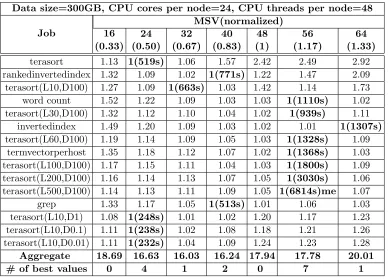
Table 4.3: Normalized performance the best completion time (in parentheses) for different MSVs on cluster P6 with 300GB data size.

Job

MSV(normalized)

16 24 32 40 48 56 64

(0.33) (0.50) (0.67) (0.83) (1) (1.17) (1.33)

terasort 1.13 1(519s) 1.06 1.57 2.42 2.49 2.92

terasort(L10,D100) 1.27 1.09 1(663s) 1.03 1.42 1.14 1.73

word count 1.52 1.22 1.09 1.03 1.03 1(1110s) 1.02

terasort(L30,D100) 1.32 1.12 1.10 1.04 1.02 1(939s) 1.11

invertedindex 1.49 1.20 1.09 1.03 1.02 1.01 1(1307s)

terasort(L60,D100) 1.19 1.14 1.09 1.05 1.03 1(1328s) 1.09

terasort(L100,D100) 1.17 1.15 1.11 1.04 1.03 1(1800s) 1.09

terasort(L200,D100) 1.16 1.14 1.13 1.07 1.05 1(3030s) 1.06

terasort(L500,D100) 1.14 1.13 1.11 1.09 1.05 1(6814s)me 1.07

grep 1.33 1.17 1.05 1(513s) 1.01 1.06 1.03

terasort(L10,D1) 1.08 1(248s) 1.01 1.02 1.20 1.17 1.23

terasort(L10,D0.1) 1.11 1(238s) 1.02 1.08 1.18 1.21 1.26

terasort(L10,D0.01) 1.11 1(232s) 1.04 1.09 1.24 1.23 1.28

Aggregate 18.69 16.63 16.03 16.24 17.94 17.78 20.01

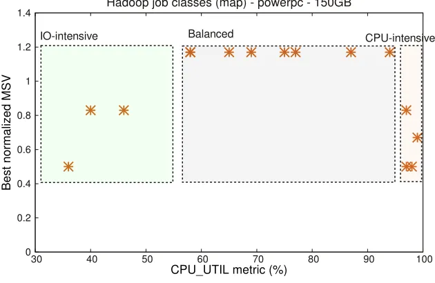
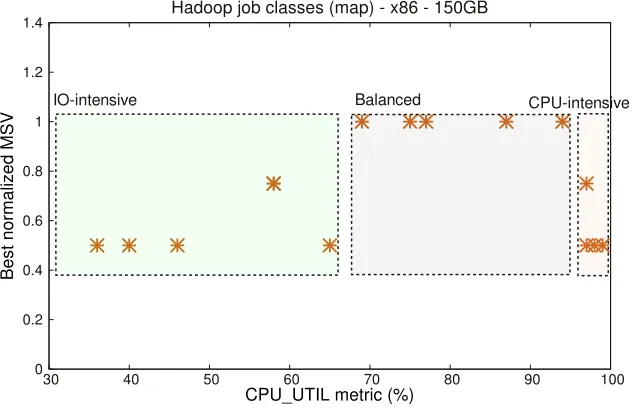
medium CPU UTIL (60% to 90%). The normalized best MSVs of applications in this region are greater than 1.0. CPU-intensiveregion has applications with high CPU UTIL (90% to 100%). Applications in this region have low IO UTIL. The best normalized MSVs of applications in this region are less than 1.0. The normalized best MSVs greater than 1.0 means that the number of map tasks exceeds the number of CPU threads in the system. This indicates that the applications are scalable. On the other hand, the best normalized MSVs less than 1.0 indicate that the applications are not scalable and face resource bottlenecks. The scalable nature of Balanced region and the bottlenecks of IO-intensive and CPU-intensive regions are described with examples in the following paragraphs.

Figure 4.3 shows the CPU UTIL against the best normalized MSV for I6 cluster. The prediction for I6 cluster is similar to the P6, except the difference in region boundaries. The IO throughput of a x86 node and a PowerPC node is 40MB/s and 100MB/s respectively.2 Due to this reason, applications with medium CPU UTIL, which in turn have medium IO THRPUT, suffer from IO bottleneck in the x86 cluster whereas they do not suffer from IO bottleneck in

2

(41)

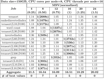
Table 4.4: Normalized performance the best completion time (in parentheses) for different MSVs on cluster I6 with 150GB data size.

Job

MSV(normalized)

4 8 12 16 20 24

(0.25) (0.50) (0.75) (1) (1.25) (1.5)

terasort 1.14 1(2688s) 1.05 1.11 1.34 1.46

rankedinvertedindex 1.09 1(1676s) 1.11 1.24 1.35 1.44

terasort(L10,D100) 1.13 1(2172s) 1.09 1.21 1.31 1.44

word count 1.88 1.04 1(1337s) 1.17 1.12 1.21

terasort(L30,D100) 1.39 1.12 1(2670s) 1.05 1.11 1.42

invertedindex 2.36 1(509s) 1.09 1.41 1.95 2.13

terasort(L60,D100) 1.24 1.24 1.01 1(2732s) 1.17 1.41

termvectorperhost 1.56 1.10 1.09 1(536s) 1.13 1.20

terasort(L100,D100) 1.61 1.29 1.14 1(2871s) 1.23 1.40

terasort(L200,D100) 1.54 1.18 1.13 1(3114s) 1.11 1.21

terasort(L500,D100) 1.85 1.25 1.16 1(3960s) 1.09 1.27

grep 1.57 1.12 1(352s) 1.05 1.09 1.10

terasort(L10,D1) 1.04 1(883s) 1.05 1.08 1.06 1.07

terasort(L10,D0.1) 1.03 1(884s) 1.03 1.09 1.11 1.13

terasort(L10,D0.01) 1.07 1(871s) 1.08 1.10 1.12 1.13

Aggregate 21.5 16.34 16.09 16.51 18.29 20.02

# of best values 0 7 3 5 0 0

the P6 cluster. As a result, the applications with medium CPU UTIL belong to IO-intensive region of I6 cluster instead ofBalancedregion. Additionally, as these applications with medium IO THRPUT have relatively higher CPU UTIL values, the Balanced region starts at a higher CPU UTIL value in the I6 cluster. This is observed in Figure 4.3. From the figure, we observe that the Balancedregion starts at 69% which is relatively higher than 58% for PowerPC.

4.2.1 CPU and IO behavior

Figures 4.4, 4.5, and 4.6 show the CPU and IO behavior of a tasktracker node for an application of each region. The figures show the node behavior including the completion time for all MSVs and help to explain the performance of an application when MSV is the best. In the figures, the CPU utilization is divided intouser,system, andiowait states. The useris the time spent by the map tasks, thesystemis the time spent by the kernel, and the iowaitis the time spent waiting for the IO operation to complete. Each figure is described as follows.

(42)

IO-intensive Balanced CPU-intensive

Figure 4.2: Classification for applications running on P6 cluster.

that beyond 24 MSV, increasing parallelism merely increases IO pressure and overhead due to the IO pressure. This explains the lower relative best MSV for applications in IO-intensive region.

Figure 4.5 shows the node behavior of invertedindex, which falls in Balanced region. The figure shows 56 as the best MSV. In Figure 4.5, theuserCPU increases until MSV is 56. After 56, the userCPU levels off without showing performance improvement. IO throughput on the other hand is almost constant and does not peak, which suggests a lack of IO bottleneck. Due to this reason, there is not any noticeable iowait. This behavior results in the applications having best MSV greater than the number of CPU threads.

Figure 4.6 shows the node behavior ofgrep, which falls inCPU-intensiveregion. The figure shows 40 as the best MSV, which is 83% of the total number of virtual CPU threads. In Figure 4.6, theuserCPU steadily increases until MSV is 40. After 40, the sysCPU increases and the user CPU levels off and decreases in small amount. This suggests that due to the high CPU utilization of grep, the system overhead increases. The IO throughput on the other hand is 0.1MB/s for all MSVs.

4.3 Performance analysis

(43)

IO-intensive Balanced CPU-intensive

Figure 4.3: Classification for applications running on I6 cluster.

Table 4.5: Aggregate normalized performance values and maximum slowdown percentages (in-side parentheses) for the three tested cases.

MSV selection PowerPC x86

150GB 300GB 150GB

Best single MSV 16.10(20%) 16.03(13%) 16.09(16%) Predicted MSV using the

regions

15.19(6%) 15.21(6%) 15.50(11%)

(44)

302s

258s 263s 304s

488s 599s

648s

Figure 4.4: CPU utilization, IO throughput, and completion time (shown in relative vertical heights) of an IO-intensiveapplication (terasort).

973s _750s _750s

657s 676s _620s _632s

Figure 4.5: CPU utilization, IO throughput, and completion time (shown in relative vertical heights) of a Balancedapplication (invertedindex).

4.4 Chapter summary

(45)

343s

289s _257s _257s _245s 272s 341s

Figure 4.6: CPU utilization, IO throughput, and completion time (shown in relative vertical heights) of a CPU-intensiveapplication (grep).

(46)

Chapter 5

Dynamic tuning

(47)

A na¨ıve way of determining the best MSV/CCS is to exhaustively profile the completion time for all MSV/CCS values. This approach is impractical as it is a time consuming process. Rather, there are existing best practices, some that suggest manually trying several possible values [6] and others that provide a guideline to set the configuration values [17]. Our findings show that following best practices can result in under utilization of resources and longer application completion time. It is therefore desirable to have an approach that effectively utilizes system resources, ensures faster completion of applications, and automatically tunes the configuration parameters. In this chapter, we develop and evaluate dynamic tuning methods to achieve these goals.

Static tuning in Chapter 4 showed that MapReduce application performance is dependent upon its CPU and IO characteristics. Using this finding, we further investigate the relationship between system resource usage metrics and application performance. We then utilize these resource usage metric values to dynamically tune MSV/CCS by using feedback controller. A feedback controller can dynamically change MSV/CCS during the execution of an application. The system resource usage is monitored at short intervals such that any bottleneck is quickly addressed. This is aided by our implementation of suspend mechanism in YARN. When CCS is lowered, the extra containers are suspended, which reduces total number of IO requests or CPU contention. This helps to immediately eliminate bottlenecks. The efficient resource usage due to the feedback controller ensures faster completion time for applications.

There are two advantages to dynamically controlling MSV/CCS over static tuning. First, it does not require profiling. Second, the ideal MSV/CCS can change during the execution of an application. For Hadoop, compared to the best profiled MSV, our approach achieves a performance improvement as high as 5% with warm start and performance loss of only 4.6% with cold start. For YARN, our findings show that our approach achieves more efficient resource usage and performance improvement of as much as 28% and 60% respectively when compared to the best practice and the default settings.

5.1 Resource usage monitoring

(48)

phase. The combine phase is optional and, when present, the map task performs a local reduce operation on the output key-value pairs. At the end, if there are multiple spill files then they are merged together to produce a single map output file. This is the merge-spill phase. Each map task phase is either CPU or IO intensive. The CPU intensive phases are compute, collect, sort, and combine. The IO intensive phases are spill and merge-spill.

Performance metrics can be collected from two different sources, which are Hadoop specific counters and the system statistics generated by an operating system in /proc/stat file for Linux. Each of them has advantages as well as disadvantages. Hadoop counters have advantage of being internal to Hadoop, with information available on processed data and the time spent by a task for compute and IO. Counters are suitable for characterizing applications as we have done in our previous work [56] and explained in this dissertation in the previous chapter. The disadvantage of using counters is the difficulty in correlating them with fine grained best MSV selection. For example, to know the extent of delay due to increased IO pressure, the counters at best can provide information on longer durations for IO operations of map tasks. But it requires extensive profiling to know what duration indicates increased delay due to IO pressure. However, metrics collected from/proc/stathave an advantage of providing such fine grained information. Operating system statistics are more general and provide instantaneous information on CPU utilization, IO read and writes, context switches, blocked processes, and other system statistics [25]. procs blocked is a metric provided by/proc/stat that shows the number of processes blocked due to IO pressure in the system. This information can then be used to determine the extent of IO pressure and thus helps in acting quickly to alleviate the IO bottleneck. The disadvantage of using /proc/statis that it requires a system call to read the metric values. Our observation during this work did not show any noticeable difference in map completion time when collecting the metrics from /proc/stat. Therefore, we use the metrics collected from /proc/stat because their advantages outweigh that of Hadoop counters when using them for dynamic control of MSV/CCS.

(49)

30-second sampled value of the measured metrics. For example, if an application runs for 1200 seconds for an MSV setting, then there are 40 resulting points each representing a 30-second sampled value. The map completion time for all these points is equal to the total runtime, which in this example is 1200 seconds. This time value is normalized in the plot with respect to the best map completion time of that application for all measured MSV values. As the y-axis is completion time, lower is better. A higher map completion time indicates bad performance whereas a smaller time indicates good performance. If a point has a lower y-axis value then that point represents the metric value resulting in good performance, whereas if a point has higher y-axis value then it represents degraded performance.

The figures do not show a correlation between the metric values and the map completion time. For example, in Figure 5.1b, a singleiowait value is mapped to multiple map completion times. This observation can be seen for alliowaitvalues throughput its range. Similar observa-tions can be made for the remainder of the metrics –system,procs running,readrate,writerate, and timeio.

In contrast, Figure 5.2a, 5.2b, and 5.2c, which show the plots foruser cpu,procs blocked, and ctxt, show some correlation with the map completion time.user cpurepresents the percentage amount of time spent by CPU in user mode, procs blockedrepresents the number of processes blocked during IO, andctxtrepresents the number of context switches performed by the system. In case ofuser cpuin Figure 5.2a, when user cpuhas a high value, the map completion time is low, but for smaller user cpu, the map completion time is ambiguous with low to high values. Figure 5.2b shows that when procs blockedhas a high value, the map completion time is high, but for low procs blockedthe map completion time is ambiguous with low and high values. In summary, these three figures show that a higher user cpu indicates good performance, higher procs blockedindicates poor performance, and a higherctxtindicates good performance. A small range in the high value results in bad performance for context switches. However, none of the metrics correlate with the completion time over the entire range of their values.

(50)

system

map completion time

(a) system time vs. normalized map time

iowait

map completion time

(b) iowait time vs. normalized map time

procs_running

map completion time

(c) running processes vs. normalized map time

readrate

map completion time