A Stationary Stochastic Approximation Algorithm for Estimation in the GLMM

(1)

CHANG, SHENG-MAO. A Stationary Stochastic Approximation Algorithm for Estimation in the GLMM. (Under the direction of Dr. John F. Monahan.)

(2)

by

Sheng-Mao Chang

A dissertation submitted to the Graduate Faculty of North Carolina State University

in partial fullfillment of the requirement for the degree of

Doctor of Philosophy STATISTICS

Raleigh, North Carolina 2007, May

APPROVED BY:

Dr. John F. Monahan Dr. Bibhuti Bhattacharyya

Chair of Advisory Committee

(3)

Dedication

(4)

Biography

(5)

Acknowledgements

I would like to thank the members of my advisory committee for their helpful and constructive advice.

I am extremely grateful to my advisor Prof. John F. Monahan for his knowl-edgeable guidance, unlimited patience, and priceless time. Every time we met, I feel inspired. On the wall of my “Free Expression Tunnel”, there is no complain but many thanks to him. I firmly believe that he is the blessing from the God that leads me to fulfill my faith.

I would like to say thank you to Dr. B.B., Dr. Boos, Dr. Davidian, Dr. Tsiatis, Dr. Genton and Dr. Zhang for their wonderful teaching. In addition, I would like to show my sincere appreciation to Dr. Stefanski and Dr. Lindsay because they changed the way I look a problem. Most importantly, I appreciate Dr. Zeng for his motivating direction and long term financial support. Without his help, I can not complete this long journey.

I also appreciate Dr. Jung-Ying Tzeng for her advice and encouragement during my most depressed days. Her support really made a remarkable change of my life. A special appreciation should go to my dear friends from Taiwanese Student Association. The friendship they provide to me is more precious than ever. Finally, I would like to thank my parents, my grand mothers and my sister for their endless love.

(6)

List of Tables

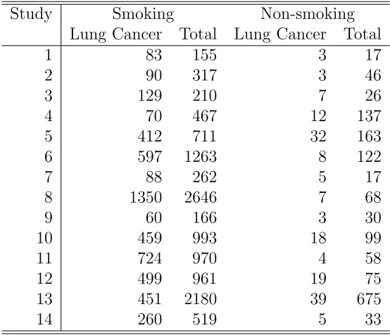
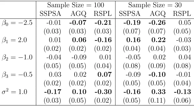
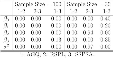
1.1 Lung Cancer Data, Booth and Hobert (1999) . . . 2 5.1 Mean Bias and Empirical Standard Error of Normal-Normal Model . 56 5.2 Mean Square Error (×100) of Normal-Normal Model . . . 56 5.3 Multiple Comparisons with Control of N-N Model: p-values of Testing

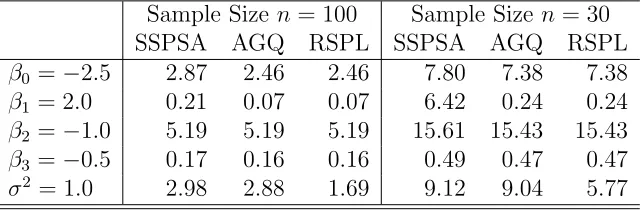
No Difference among Parameter Estimates . . . 57 5.4 Mean Bias and Empirical Standard Error of Logistic-Normal Model . 60 5.5 Mean Square Error (_×100) of Logistic-Normal Model . . . 60 5.6 Pairwise Multiple Comparisons of L-N Model: p-values of Testing No

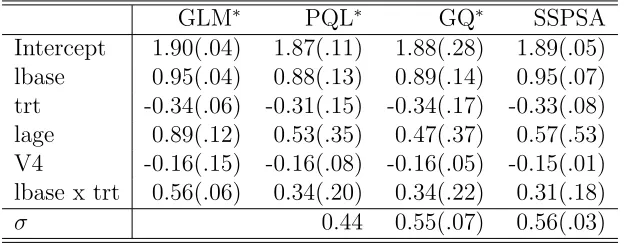
Difference of Parameter Estimates . . . 61 5.7 Summary Results, Parameter Estimates (Standard Errors), for Epilepsy

Seizure Data . . . 62 5.8 Summery Results, Parameter Estimates (Standard Errors), for Lung

Cancer Data . . . 63 5.9 Summary Results, Parameter Estimates (Standard Errors), for

(9)

List of Figures

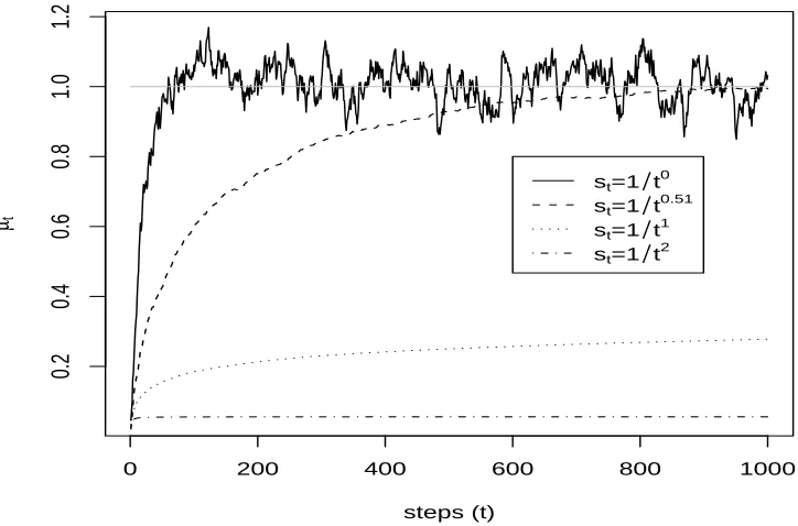
4.1 Effect of step size st on SPSA sequences. . . 38

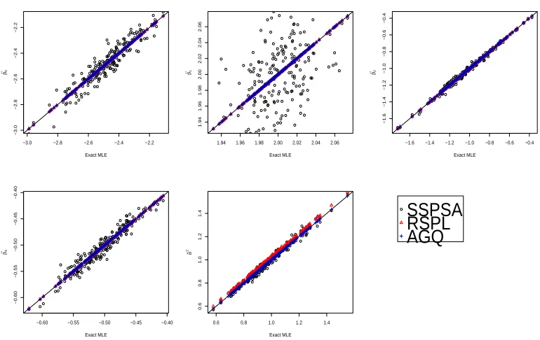
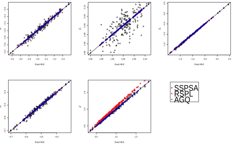
5.1 N-N model, sample size 100: Comparisons of three methods: SSPSA, AGQ and RSPL. Exact MLEs versus approximated MLEs are plotted. 57 5.2 N-N model, sample size 30: Comparisons of three methods: SSPSA,

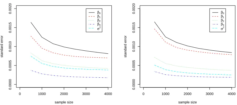
AGQ and RSPL. Exact MLEs versus approximated MLEs are plotted. 58 5.3 N-N model, n = 100 (Left) and n = 30 (Right): Variation due to

SSPSA with different numbers of iterations . . . 59 5.4 L-N model, n = 100 (Left) and n = 30 (Right): Variation due to

SSPSA with different numbers of iterations . . . 61 5.5 Lung cancer data: Monte Carlo log-likelihood surface of σ2

u and σv2

when (β0, β) = (−1.9,1.7). . . 64 5.6 SSPSA sequences for Salamander Mating Data with initial value

pro-vided by Gibbs estimate, Zeger and Karim, 1991 . . . 65 5.7 Monte Carlo marginal likelihood with (Left) SSPSA and with (Right)

Gibbs fixed-effect coefficient estimates. . . 66 B.1 The ξ2

(10)

Chapter 1 Introduction

The generalized linear mixed model (GLMM) has served as a useful tool to sci-entific discovery. This kind of model consists of a response following a distribution belonging to the exponential family, a link function, and covariates with random and/or fixed coefficients. Through the assigned link function, the conditional mean of the response is a function of a linear combination of covariates. Following are some examples:

• Epileptic Seizure Data (Thall and Vail, 1990) In a clinical trial, 59 epileptic patients were randomly assigned to have new drug or placebo (treatment). The response is the number of seizures among 4 clinics and the covariates are: base line seizures, age, and, of course, the treatment. In addition, it is reasonable to assume that individuals have different reactions to different treatments. With multiple observations on each individual, thus random effect can be identified and estimated.

(11)

incidence of lung cancer, evidence presented in Section 5.2.2 suggests a random study effect.

• Salamander Data McCullagh and Nelder (1989) reported an interesting dataset which contains information about the mating preference of two isolated salamander populations. Each female individual was assigned to mate with three males which may or may not be in the same population. The mating design is not balanced in order to avoid time effects. Since there are three measurements (successfully mated or not) per individual it is reasonable to take individual effects into account. Again, individual effect is assumed to be random.

In all of these examples the response variable is discrete and the model contains random effects.

Table 1.1: Lung Cancer Data, Booth and Hobert (1999)

Study Smoking Non-smoking

Lung Cancer Total Lung Cancer Total

1 83 155 3 17

2 90 317 3 46

3 129 210 7 26

4 70 467 12 137

5 412 711 32 163

6 597 1263 8 122

7 88 262 5 17

8 1350 2646 7 68

9 60 166 3 30

10 459 993 18 99

11 724 970 4 58

12 499 961 19 75

13 451 2180 39 675

14 260 519 5 33

(12)

ex-ponential family whose mean is a one-to-one function of the linear combination of covariates (or predictors or independent variables.) For example, in the seizure data, a simplified model of Breslow and Clayton (1993) is considered. The response yij is

the number of seizures of patient i at the jth visit to a clinic. It is reasonable to assume yij follows Poisson distribution with mean µij and

logµij =XTijβ+ui,

where Xij is a vector containing the fixed effect covariates, β representing the

corre-sponding unknown coefficient, and intercept andui denoting the individual variation

of individual i. The random variable uj’s are normally distributed with a common

variance.

In the lung cancer data, for the study i and smoking group j (j = 1 if smoking and j = 0 if non-smoking), the response follows the binomial(nij, pij) distribution

with the link function log(pij/(1−pij))≡logit(pij) =β0+β1xij +ui+vij. Here, xij

indicates the smoking statusj of studyi;ui represents the random variation of study

i; vij denotes the random effect of smoking status j within study i. Note that β’s

stand for the coefficients of fixed effects and ui’s andvij’s follow normal distributions

with mean zero and unknown variance.

In the salamander data, Karim and Zeger (1992) proposed the random effects model as follows

logit(Pr(Yij = 1|Xij, ufi, umj )) =XTijβ+u f i +umj

where the vector X_ij indicates the population of two individuals, the ith female and the jth male, and the uf_i and um

j represent the corresponding individual effects.

Without further information, we assume uf_i ∼ N(0, σ2

f), umj ∼ N(0, σm2) and mutual

independence among individuals.

(13)

likelihood of the ith individual has the form

Li(γ,D) =

Z

Rq

p(yi|Wi,u;γ)dΦ(u;0,D) (1.1)

where p(·|Wi,u;γ) denotes the density function of the response, usually belongs

to exponential family, u follows a q₋dimensional multivariate normal distribution with mean zero and variance Dq×q, and γ is a vector of parameters. The response

is yi and Wi is a row vector of covariates which corresponds to the ith individual.

Throughout this work, we reserveφ(·;µ,Σ) and Φ(·;µ,Σ) to denote the normal density and distribution function, respectively, with meanµand variance-covariance Σ. Both γ and D are unknown parameters. For convenience, denoteθT _{= (γ}T_{, vec(D)}T_{). The}

linear relationship is characterized by

E(Yi|Wi,u) =µi and η(µi) = XTi βp×1+ZTi uq×1

whereWn×(p+q)= [Xn×p,Zn×q],Wi is theith row ofW, andη(·) is the so-called link

function in the generalized linear model literature. Additionally, the link function should be one-to-one and be pre-specified before analysis.

The remainder of this work is arranged as follows. In Chapter 2, we review the literature of GLMM, begining with the LMM and then show the difficulties in its gen-eralized version GLMM. Several major approaches are mentioned, including approxi-mate integral, approxiapproxi-mate integrand, and EM. In Chapter 3, we review the literature on stochastic approximation (SA). SA is designed for root finding or optimization of

anon-deterministicobjective function. Several of its extensions are reviewed as well.

(14)

(15)

Chapter 2 A Review of GLMM

The most well studied subclass of GLMMs is the linear mixed model (LMM) – replacing p(·) by φ(·) in (1.1) and taking the link function as identity, i.e. η(x) =x. For a detailed survey, we refer to Verbeke and Molenberghs (2001) and McCulloch and Searle (2001). Similar conjugate classes in the statistical literature are the Beta-binomial model (Lee and Nelder, 1996), Poisson-Inverse Gamma model (Breslow, 1984), and other over-dispersion models. A favorable feature of these models is that their marginal likelihood has a closed form so the MLE is tenable by taking derivatives. On the contrary, if p(·) in (1.1) is chosen so that the corresponding integral has no closed form then approximations or numerical methods are required. Several popular solutions are examined below. Note that most of leading methods are combination of them.

(16)

2.5, Bayesian and non-fully-parametric methods are briefly mentioned.

2.1 Linear Mixed Model

The linear mixed model can describe a variety of statistical problems such as analysis of variance (Searle et al. , 1991), longitudinal experiment (Verbeke and Molenberghs, 2001), linear models with latent variables (Fuller, 1987), and others. In this section, we consider its general formulation and the construction and merits of restricted maximum likelihood estimate (REML). These ideas remain important in GLMM inference and computation.

2.1.1 General Formulation

The linear mixed model can be defined as y = Xβ + Zu+ ǫ where ǫn×1 ∼ N(0,Rn×n),uq×1 ∼N(0,Dq×q) andǫanduare independent. Note that, (yn×1,Xn×p,

Z_n_×_q) is defined as before;βp×1 denotes the fixed effect coefficient vector whereasuq×1 denotes the random effect coefficient vector. Taking advantage of conditional expec-tation, we have

Thus, we haveY follows normal distribution with meanXβand varianceR+ZDZT. It turns out that, analogous to (1.1), the marginal likelihood is

(2π)−n/2|R+ZDZT_|−1/2exp

−1

2(y−Xβ)

T_(R₊_ZDZT₎−1_(y₋_Xβ)

.

Although the marginal likelihood is simple, deriving the maximum likelihood estima-tor (MLE) can be complicated. A detailed derivation can be seen from Wolfingeret al.

(17)

2.1.2 Restricted Maximum Likelihood

In random effect methods, sometimes we are more interested in the variance com-ponents, D and R, rather than the other parameters, γ. Suppose that variance components are our major interest so we can treat the fixed effect coefficient β as a nuisance parameter. One way to deal with the nuisance parameter is projecting the model onto a subspace so that the estimation of β does not affect the estimation of variance components. For example, let K_n_×_n be a real matrix such that

Ky =KXβ+KZu+Kǫ=KZu+Kǫ,

and KXβ = 0 for all β _∈ _Rp_{. Then the distribution of} _Ky _{is normal with mean}

0 and variance KZDZTKT +KRKT, free of β. The ML inference using this kind of transformed model is called REML, Thompson (1962). A possible K is I_n₋P_X where PX = X(XTX)−XT, where “−” denotes a generalized inverse. It turns out

that the transformed response

Ky = (I₋P_X)y

is exactly the residual of linear regression with fixed effects only. So the “RE” in REML stands for the “residual” as well.

(18)

2.2 GLMM: Approximate Integral

The first solution is to approximate the integral in (1.1). We review three ap-proaches. First, one may approximate the integral with fixed abscissas such as trap-zoid rule, Simpson’s rule, and Gaussian quadrature (GQ). This kind of approximation usually has low errors but it is not unbiased and it is not easy to control the accuracy. We introduce GQ in Section 2.2.1. Second, one may construct an unbiased estimator of the integral,e.g. , Monte Carlo (MC) and importance sampling. This kind of esti-mation is unbiased and the corresponding variance is easy to derive, see Section 2.2.2. However, the convergence rate of MC is slow. The third possibility is combining the above two together, e.g. , the Radial-Spherical (RS) method, and thus, inheriting those merits at the same time, see Section 2.2.3. In the following, we are going to introduce these three major methods to approximate or to estimate the integration. Hereafter, denote pi(u) as the shorthand of p(yi|Wi,u;D) if there is no confusion.

2.2.1 Gaussian Quadrature Approximation

Gaussian quadrature (or Gauss-Hermite quadrature) serves as an approximation of the integral having the form

Z

R

f(z)e−z2/2dz (2.1)

where f(_·) is a smooth function. The mth order GQ approximation is defined as

m

X

j=1

wjmf(zjm)≈

Z

R

f(z)e−z2/2dz (2.2) where _{zjm} are roots of mth order Hermite polynomial and {wim} are suitable

weights. This approximation is useful, in particular, when the integral has the form like (1.1). Consider (1.1) with one-dimensional u_∼ N(µ, σ2_{) for example. Let} z = (u₋µ)/σ. The likelihood in (1.1) can be rewritten as

Li =

1

√

2π

Z

R

pi(σz+µ)e−z

2_/₂

(19)

so GQ can be applied directly. For a more general class like R g(x)dx, g : R → R, one can also apply GQ to approximate the integral (Liu and Pierce, 1994). A general form is as follow:

Z

g(x)dx=

Z

g(x)

φ(x;µ, σ2₎φ(x;µ, σ

2_)dx₌

Z

g(µ+σz) φ(z; 0,1) ×

1

√

2π ×e

−z2_/₂

dz.

So we go back to the form of (2.1) and hence, weights {wj}’s in (2.2) are still valid.

In practice, the random variable x usually has higher dimension. Fortunately, the GQ technique remains similar; simply apply the product rule. For example, let z= (z1, z2)T _and _f _:_R2 _→_R _{then the corresponding GQ has the form}

Z

R2

f(z)e−zTz

dz_≈

n

X

i=1

m

X

j=1

winwjmf(zin, zjm)

where _{zin, zjm}’s are relevant abscissas and{win, wjm}’s are corresponding weights.

If the d−dimensional random variable u follows a normal distribution with mean µd×1 and variance Dd×d which is positive definite, then the relevant transformation

is z = L−1(u−µ) where D =LLT is the Cholesky decomposition and L is a lower triangular d_×d matrix. Consequently,

Z

Rd

pi(u)φ(u;µ,D)du=

Z

Rd

pi(Lz+µ)φ(z;0,I)dz.

For a general introduction and implementation, we refer to Monahan (2001) and for a detailed treatment, we refer to Davis and Rabinowitz (1984).

(20)

2.2.2 Monte Carlo Approximation

A straightforward method of approximating an integral is MC integration. That is, sample u_j’s i.i.d. Φ(u;0,D) so that the sample mean gives

1 m

m

X

j=1

pi(uj)≈

Z

pi(u)dΦ(u;0,D).

According to the strong law of large numbers, the left-hand side converges to the right-hand side. If sampling from φ(·) is difficult or inefficient, then importance sampling can be used. With importance density g(_·), the approximation becomes

1 m

m

X

j=1

pi(uj)

φ(uj; 0,D)

g(uj)

so that

E

(

1 m

m

X

j=1 pi(uj)

φ(uj; 0,D)

g(uj)

)

=

Z

pi(u)dΦ(u;0,D)

where the uj’s are i.i.d. samples having density function g(·). The choice of g(·) is

crucial. At a minimum, samples need to be drawn from it andg has to be absolutely continuous with respect to φ. In practice, when the underlying distribution is normal a Student−t distribution can be the importance distribution which provides a more robust result (although it is not the most efficient choice), Evans and Swartz (1996). Other choices for sampling efficiency and practical issues can be seen in Srinivasan (2002). For references discussing GLMM and nonlinear mixed model with approxi-mate likelihood, we refer to Durbin and Koopman (1997), Pinheiro and Bates (1995), and references therein.

(21)

algorithm have been successfully proposed as solutions of GLMM problem (see Chen

et al. , 2002, for example.) Among these methods, the efficiency of algorithms is

rooted in the sample size drawn from the underlying sampler. We will come back to this issue when we discuss the EM algorithm.

As Monahan and Genz (1997) pointed out in a d−dimensional integration prob-lem, the numerical quadrature may converge with rate O(m−2/d_{) or} _O(m−4/d_{) where}

mis the number of abscissas, whereas the MC method converges withO(n−1/2_{) where} n represents the number of function evaluation. The curse of dimensionality operates on fixed quadrature severely but not on the MC. The other drawback of quadrature is the difficulty of evaluating its accuracy. An idea that fuses GQ and MC together has been proposed by Siegel and O’Brien (1985) and Genz and Monahan (1998). We demonstrate this idea in next subsection; however, we refer Chapter 12 of Monahan (2001) for a detailed treatment.

2.2.3 Radial-Spherical Approximation

Consider integrating the function f : [0,1]_→_R using

ˆ If =

1 n

n

X

i=1 f

U+ i−1 n

whereU follows a uniform distribution at interval [0,1/n]. Now, since ˆIf is a random

variable, we have

EU[ ˆIf] =

1 n

n

X

i=1

Z 1/n

0

n_×f

u+i−1 n

du=

Z 1

0

f(v)dv.

In words, ˆIf is an unbiased estimator of

R1

0 f(v)dv. Together with the idea of quadra-ture, Siegel and O’Brien (1985) suggested an unbiased integral rule which integrates over the interval [−1,1]:

(22)

where (w0(R), w1(R)) = (2−2/3R2_,_1/3R2_{) and} _R _{has the density function 3r}2 _on [0,1]. For any function f, Tf(R) is unbiased, i.e. ERTf(R) =

R1

−1f(r)dr and Tf(R) is exact if f is a cubic polynomial.

Further, Genz and Monahan (1998) proposed another integral rule Mk

f(R) which

is an unbiased estimator of 2−d/2 Γ(d/2)

Z ∞ −∞

f(r)_|r_|d−1e−r2/2dr (2.3) where the superscript of M denotes the degree of rule. Take the third-order rule for example. Let R _∼ χd+2 and weights w0(R) = 1−d/R2 and w1(R) = d/4R2. So M3

f(R) has the form

M_f3(R) = w0(R)f(0) +w1(R)(f(R) +f(₋R))/2.

Formulas for the wi’s are given in Genz and Monahan (1998) for variousk.

The other useful integral rule is for the integration over the surface of thed₋dimensional unit ball denoted as Ud. Stewart (1980) proposed an efficient algorithm to compute

a random orthogonal matrix Q such that

Z

Ud

f(z)dz= E

" _k X

i=1

uif(Qv(i))

#

(2.4)

wherev(i) denotes theith abscissa (ad−dimensional vector) andui is its

correspond-ing weight. SupposeXis a matrix where each element inX is a random sample from standard normal distribution. Its QR decomposition can be denoted as X = Q1R1 where columns of Q₁ are orthogonal and R₁ is upper triangular. Then, Q₁ is a valid random matrix ofQfor radial-spherical approximation. Actually,Qrandomly rotates v(i)’s so that the weighted sum (2.4) becomes a random variable and is unbiased.

(23)

(d−1)−dimensional,

Z

Rd

g(u)φ(u)du=

Z

R+

Z

Ud

g(rz)φ(rz)dzrd−1dr.

Obviously, the inner integral can be approximated by (2.4) and the outer can be approximated by (2.3). This suggests that the inner integral can be estimated by

Gn1(r) =

1 n1

n1

X

j=1

k1

X

i=1

uig(rQ(j)v(i))φ(rQ(j)v(i))

and thus, the estimator for the whole integration becomes 1

n2

X

j=1

kX2−1

i=0

wi(rj)(Gn1(rj) +Gn1(−rj))/2.

As suggested by Monahan and Genz (1997), a better approximation is a mixed RS approximation: adopting (2.4) for estimating the inner integral and using GQ for the outer integral. Clarkson and Zhan (2002) implemented GLMM fitting by the mixed RS approximation. To sum up, RS approximation is very efficient and precise as long as the integrandg is smooth or symmetric.

2.3 GLMM: Approximate Integrand

In this section, we consider methods that replace g by its approximated version ˆg in (1.1) so that the integral has a closed form. Popular choices are penalized quasi-likelihood (PQL) and pseudo-quasi-likelihood (PL). For logistic regression with a random effect, we describe the the logistic-normal approximation. Next, we review these methods and investigate how they work.

2.3.1 Penalized Quasi-Likelihood

(24)

of a locally quadratic approximation of the integrand and the Laplace approxima-tion. The approximated likelihood can be derived by following steps. First, we define p(u) = exp{k(u)} and expand k at u∗ where ∂k(u)/∂u|u₌u∗ = 0, i.e. u∗ is the

maximum. By doing so, we can define ˆ

p(u) = exp

k(u∗₎₋1

2(u−u

∗₎T_K∗_(u₋_u∗₎

where

K∗ = ₋∂ 2_k(u) ∂u∂uT _u =u∗ .

Then, PQL approximates (1.1) by replacing pi by ˆpi and consequently, the

approxi-mated version of (1.1) becomes

Z

ˆ

p(u)φ(u;0,D)du

∝p(u∗₎_|_D_|−1/2

Z

exp

−1

2(u−u

∗₎T_K∗_(u₋_u∗₎₋1

2u

T_D−1_u

du

=p(u∗₎_|_D_|−1/2

Z

exp

−1

2u

T_(K∗ ₊_D−1_)u₊_u∗T_K∗_u

du

where _|A_| denotes the determinant of matrix A. In order to make the integrand a Gaussian kernel, let A = I + K∗−1/2D−1K∗−1/2 and rewrite the exponent as

−1/2uT_K∗1/2_AK∗1/2_u₊_uT_K∗1/2_A1/2_A−1/2_K∗1/2_u∗ _{and thus}

Z

ˆ

p(u)φ(u;0,D)du

∝p(u∗)|D_|−1/2_|D−1+K∗_|−1/2exp

−1

2u

∗T_(D₊_K∗−1 )−1u∗

.

(2.5)

This procedure is also called the Laplace approximation of order two.

Although (2.5) is elegant, it can be expected that when the second-order Taylor expansion performs badly, the approximation fails to mimic (1.1) closely. From an-other viewpoint, ˆpi(u) is proportional to the normal distribution with mean u∗ and

variance K∗−1. Thus, the condition that PQL performs well is that pi(u) acts like

(25)

and Lin (1995) and Lin and Breslow (1996) proposed a fourth-order Laplace ap-proximation in order to reduce biases. Raudenbush, et al. (2000) provided a general framework for higher-order Laplace approximation. They showed that the sixth-order Laplace approximation is very competitive to AGQ where the number of abscissa is chosen empirically.

2.3.2 Pseudo-Likelihood

In the GLMM literature, pseudo-likelihood (PL) method, Wolfinger and O’Connell (1993), is a popular alternative to PQL. We quote Carroll and Ruppert (1988) to explain the PL idea:

Pseudo-likelihood estimatesθare based on pretending that the regression parameter β is known and equal to the current estimate ˆβ∗ and then

estimating θ by maximum likelihood assuming normality.

Wolfinger and O’Connell (1993) defined the pseudo-response as follows. Let E(Y|u) = µ = η−1_{(ν) where} _ν

n×1 = Xβ +Zu. Note that η−1(·) denotes the inverse function of η(·), not the reciprocal. With relevant initial values ( ˆβ,u) we further define ˆˆ ν = Xβˆ+Zˆu. The first order Taylor expansion of η−1_{(ν) with respect to ˆ}_ν _yields

η−1(ν)_≈η−1(ˆν) + ˆBX(β₋β) + ˆˆ BZ(u₋u)ˆ (2.6) where ˆB=∂η−1_/∂ν_|

ν=ˆν is an n×n diagonal matrix. Rearranging (2.6) yields

ˆ

B−1(µ−η−1(ˆν)) +Xβˆ+Zˆu_≈Xβ+Zu

where the left-hand side of above equation is the (conditional ) expectation of P= ˆB−1(Y₋η−1(ˆν)) +Xβˆ+Zu.ˆ

(26)

2.3.3 Logistic-Normal Approximation

DenoteGandgas the distribution and density function of the logistic distribution. Andrews and Mallows (1974) and Stefanski (1990) showed that

G(z) =

Z ∞

0

Φ(z/σ)q(σ)dσ where q(σ) =dL(σ/2)/dσ and

L(σ) = 1₋2

∞

X

j=1

(₋1)j+1exp_{−2j2σ2_}

is the Kolmogorov-Smirnov distribution. In words, a logistic distribution is a mixture of scaled normals. This motivates using a finite sum of weighted scaled-normal densi-ties to approximate a logistic density. Monahan and Stefanski (1992) introduced this method to GLMM and measurement error model.

Similar to GQ, they approximated G(z) by G∗

k(z) = k

X

j=1

wjΦ(sjz), k= 1,2, ...

where, for a fixedk, the pairs (wj, sj) are chosen so that the error ∆k = supz|G∗k(z)−

G(z)_| is minimized. Monahan and Stefanski (1992) provided a table for the pairs (wj, sj) from k = 1 tok = 7 and also showed the corresponding errors. Consider the

ith-observation marginal likelihood of logistic regression with normal random effect

Li =

Z

R

G(µi)yi(1−G(µi))1−yidΦ(u; 0,D)

where µi =Xiβ+Ziu. When yi = 1 and replacingG(·) by G∗(·), we have

L∗_i =

Z

R

k

X

j=1

wjΦ(µi; 0, s−j2)dΦ(u;0, D) = k

X

j=1

wjΦ(Xiβ; 0, s−j2+ZiDZTi )

where the second equality is due to Lemma 2.1 of Guptaet al. (2004). Consequently, the kth-order logistic-normal approximate marginal likelihood becomes

L∗_k =

n Y i=1 " _k X j=1

wjΦ(Xiβ; 0, s−j2+ZiDZTi )

#yi"

1₋

k

X

j=1

wjΦ(Xiβ; 0, s−j2 +ZiDZTi )

#1−yi

,

(27)

2.4 GLMM: EM Algorithm

The EM algorithm of Dempster, Laird, and Rubin (1977) is a powerful tool to solve missing value problems. In the context of the GLMM, u is unobserved, i.e. , missing, thus applying the EM algorithm is appropriate, see also Searleet al. (1991). In our notation, the EM algorithm can be described as follows. Define the complete data log-likelihood as

lC(γ,D) = n

X

i=1

logp(yi|Wi,u;γ) + logφ(u; 0,D).

Further, suppose θ = (γ, vec(D))T _{is the vector of unknown parameters and} _θ(t) denotes the current estimate. Then the EM algorithm is

• Expectation (E-step): calculate

Q(θ_|θt) =

Z

lC(θ)×fU_|_Y(u|y;θ_t)du (2.7)

where

fU_|Y(u|y;θ) =

φ(u; 0,D)

R Qn

i=1p(yi;Wi,u, γ)φ(u; 0,D)du .

• Maximization (M-step): evaluate

θt+1 = arg max

θ Q(θ|θt) (2.8)

• Updating: update θt by θt+1 until certain stopping criteria are met.

The EM algorithm has many merits especially that it guarantees the improvement of the likelihood after each iteration. For regularity conditions for convergence, see Dempster et al. (1977) and Wu (1983).

(28)

algorithm. Booth and Hobert (1999) pointed out that MC integration introduces extra error. This error decreases when MC sample size increases and conversely, in-creases when MC sample size dein-creases. From another viewpoint, the current value θt from MC or importance sampling is actually a random variable and thus, its

vari-ance suffices to be a measure of the error. Since the MC sample size directly affects the magnitude of the variance, researchers have proposed various ways to empirically adjust the MC sample size, e.g. McCulloch (1994, 1997) and Chan and Kuk (1997). The solution proposed by Booth and Hobert (1999) is very straightforward. Sup-pose θt+1 follows a normal distribution with mean θ∗t+1 and variance D∗t+1. If the previous step solution θt is very close to θ∗t+1, say within its 75% confidence inter-val (C.I.), then the (t+ 1)th step is meaningless since the previous solution is not significantly different from the current solution. A better way to make the update meaningful is to increase the MC sample size so that the variance is decreased. Booth and Hobert (1999) use the delta method to construct the variance estimator and ex-tend it to the importance sampling case. With the help of this variance estimate, the updating procedure becomes

• Evaluate the variance estimate Vardm(θt+1) where the subscript m denotes the current MC sample size.

• Check if θt locates within the 75% C.I. of normal distribution with mean θt+1 and varianceVardm(θt+1). If yes, then increase sample size m tom′ and then go

back to E-step and recalculate θt+1. If no, then keep the MC sample size as m

and calculate θt+2.

Booth and Hobert (1999) suggested taking m′ ₌_m₊_{m/k, for}_k _{=3, 4, or 5.}

Another important issue in the EM algorithm is the stopping rule. Denote θ(tj) as

the jth element of the vector θt. Then, a popular stopping rule is

max

j

(

|θ(_t₊₁j) ₋θ(_tj)_|

|θ_t(j)_|+δ1

)

j=1,...,d

(29)

where δ1 and δ2 is known, e.g. δ1 = 0.001 and δ2 = 0.0001 (Searle et al., 1992). Note thatδ1 is a small positive value so that the denominator can always be far away from zero. Booth and Hobert (1999) noticed that this criterion is good for GLMMs as long as there is no error in each step. Instead, they suggested using

max

j

  

|θ(_t₊₁j) ₋θ(_tj)_|

d

Var1/2(θ(_t₊₁j)) +δ1

  

j=1,...,d

< δ2 (2.10)

so that the error is taken into account. Sinceθ(t) _{always contains certain error, Booth} and Hobert (1999) suggested δ2 = 0.02; empirically, this approach performs very well. The ground-breaking idea in their paper is that given the data (y,W) the EM solutionθt aided by MC is a random variable rather than a fixed value. One can and

should take advantage of this point to improve the algorithm analogous to the EM problem with deterministic objective function.

Last, we comment on solving GLMM problem using EM algorithm. We quote words from Boos and Stefanski (2007):

The EM Algorithm is often useful when the complete data likelihood has the form of an exponential family....the M step is straightforward and basically inherited from the exponential family, but the E step is often challenging and not necessarily aided by the exponential family...

(30)

2.5 GLMM: Semiparametric, Nonparametric, and

Bayesian

Beyond those already discussed, there are still other ways to pursue a good solution to the GLMM problem. In this section, we briefly describe nonparametric methods, semi-parametric methods, and some recent-developed Bayesian methods. For brevity, all methods will be explained in the one-dimensional case, although they can be easily extended to the multivariate case.

Nonparametric methods focus on the freedom of assigning the distribution of random effect. Analogous to (1.1), we define the marginal likelihood as

Z

pi(yi|Wi, u;γ)dG(u;τ)

whereGandgdenote the distribution and density function of random variableuwith parameter vector τ. For the semi-nonparametric (SNP) model, Zhang and Davidian (2001) defined g(·) as a normal density multiplied a polynomial and divided by a norming constant. For example, a second-order SNP model can be written as

gSN P(u) = (α0+α1u+α2u2)2φ(u;µ, σ2)/C (2.11)

whereC is the norming constant. A more general class is assumingG(·) as a mixture of normals, i.e. ,

gN P(u) =

Z

φ(u;µ, σ2)dH(µ, σ2) (2.12) for some distribution function H _{∈ H} where _H is the collection of all possible dis-tribution functions of (µ, σ2_{). If the nonparametric maximum likelihood estimate is} applied, the solution exists but G must be a step function (Lindsay, 1983). Further, Magder and Zeger (1996) defined another space HS ⊂ H so that the estimated G

(_{∈ H}S) yielded from (2.12) is smooth.

(31)

on subject-specific level, GEE method concentrates on the population-average level. Therefore, the GEE may be inefficient to estimate the variance components (McCul-loch, 2003). GEE begins by assigning a marginal model for the response. The only assumption onu is that it has zero mean. Thus, the population average E(Yi|Wi) is

only the function of β but not of u. For example, in logistic regression only specify

E(Yi|Wi) = pi and logit(pi) = XTi β.

where Yi is an r-dimensional vector with correlated elementYi1, ..., Yir. The

correla-tion is caused by sharing random effects. Suppose that the correlacorrela-tion structure of Yi is denoted as V(yi). Then, by theory, the estimating equation is

X

i

∂pi

∂βTV

−1_(y

i)(yi−pi).

(32)

(33)

Chapter 3 A Review of Stochastic

Approximation

Estimation methods are often defined as the result of an optimization problem. Least squares estimation arises from minimizing the sum of squared errors. Maxi-mum likelihood (ML) is another: Parameters are chosen so that the corresponding likelihood is maximized. When the objective function, that is, the function that one want to optimize, is smooth, basic calculus theory applies: If the functionf :_Rd_→

R

has a maximum or minimum then there exists a vector θ∗ _∈_Rd _{such that}

df(θ) dθ

θ=θ∗

=g(θ∗) = 0 (3.1)

That is, if the objective function is well behaved so that the optimal point is unique,

i.e. the objective function is strictly convex or concave in Rd, then (3.1) is helpful to find the optimal point and, hence, the optimization problem is converted to a root-finding problem.

(34)

of g(θ) has the form: θt+1 =θt−

▽2f(θ_t)−1▽f(θ_t) = θ_t−[J_g(θ_t)]−1g(θ_t). (3.2)

Here ▽f is the gradient, ▽2f is the Hessian matrix, and J_g = ∂g(θ)/∂θ. It is

well-known that when f(_·) is quadratic the solution can be reached in one step from any initial valueθ0; otherwise, a good initial value is crucial for convergence. Many other methods have similar form of (3.2), e.g. steepest descent, quasi-Newton, and others (see Monahan, 2001, and Spall, 2003, for more insightful discussion.) In multivariate case, g is explained to be the best direction toward the optimal and Jg rotates and

scales the direction so that the move [Jg(θt)]−1g(θt) is optimized. However, the

com-putation of [Jg(θt)]−1 is often costly so many other remedies have been proposed in

literature. A common belief is that if the matrix [Jg(θt)]−1 is not exact then more

iterations are required.

Above, we dealt with a deterministic function f and its derivatives g and Jg.

However, in some cases, we can not evaluate them analytically but only can get un-biased evaluations, e.g. the MC and importance sampling integration are unbiased to its deterministic integral. Under this circumstance, Robins and Monro (1951) pro-posed the stochastic approximation (SA) to find the root of g(θ). Later, Kiefer and Wolfowitz (1952) defined the optimization version of SA; we called it KWSA. While both SA and KWSA originally designed for one-dimensional problems, Blum (1954) extended them to multi-dimensional problems. Recently, Spall (1992) proposed sim-ulaneous perturbation SA (SPSA) which reduces computational burden dramatically and provides some elegant large sample properties. Next, we are going to introduce these methods followed by a section about implementing SPSA on GLMM.

3.1 SA – Root Finding

(35)

error; only y(θ), a contaminated version of g(θ), is available, for every θ. More formally, the objective function for SA has the from

g(θ) = E(Y(θ)) =

Z

ydH(y_|θ)

whereH(·|θ) : [−C, C]→[0,1] is a valid distribution function for anyθ and for some C _∈R+. Moreover, assume that the derivative ofgaround the true valueθis positive. The proposed algorithm is

θt+1 =θt−styt (3.3)

where yt =y(θt) for shorthand and st → 0, P∞_t₌₁st = ∞ and P∞_t₌₁s2t < ∞. If the

derivative is negative then we change the sign in (3.3) from “−” to “+”. Note that st,

analogous to Jg(θt) in (3.2), controls the gain/step size of each iteration. Conditions

on st determine the convergence of θt. The sequence st can not decrease too fast,

otherwise the algorithm can not search the whole support of θ. At the same time, it can not be too slow or the algorithm never converges. Robins and Monro (1951) also showed that under conditions mentioned above, θt converges to the true value θT rue

in probability. In the case of a linear response function g(θ) which corresponds to simple linear regression, Chung (1954) proved that the optimal gain sequence follows

st=

s0 t0+t ×

1 b

where s0 and t0 are two positive numbers and b is the slope of regression line.

The motivating example in Robins and Monro (1951) paper is very helpful for understanding the usefulness of SA algorithm. In this paragraph, we restate their example in our words. Suppose people are interesting in simple linear regression problem

M(x) =β0+β1x

where M(x) denotes the mean response of given x. Rather than knowing β0 and β1, interest may lie in finding xα such that M(xα) = α. Note that, for a particular xi,

(36)

β1xi+ei whereei is not observable and has zero mean. Then, the SA algorithm with

the objective functiong(x) = M(x)₋αand its contaminated versiony(x) = w(x)₋α provides a consistent estimate of xα if all conditions are met. It is worth emphasizing

that this method is nonparametric since we only require the existence of a validH(_·|θ) but do not specify a particular form for it.

3.2 KWSA – Optimization

It is more common to have an optimization problem than to have a root finding problem in statistical modeling. Kiefer and Wolfowitz (1952) designed the optimiza-tion version of SA denoted as KWSA. The objective funcoptimiza-tion is

f(θ) =

Z

ydH(y|θ)

where H(_·|θ) :R→[0,1] is a valid distribution function for any θ. Moreover, if f(θ)

is Lipschitz and _Z

∞ −∞

(y₋f(θ))2dH(y_|θ)<_∞, the algorithm following the iteration step

θt+1 =θt−st

yt+−yt−

2ct

=θt−stψt

with y_t+ _∼ H(y_|θt+ct) and yt− ∼H(y|θt−ct) guarantees that θt converges to θT rue

in probability as long as following conditions are satisfied: 1) st, ct >0 and →0; 2)

P∞

t=1st=∞; 3)

P∞

t=1stct <∞; and 4)

P∞

t=1s2tc−t2 <∞.

The strategy of KWSA is using ψt = (y+t −yt−)/2ct to approximate df(θt)/dθt.

Obviously, if ψt is unbiased to df(θt)/dθt then using SA is sufficient. Since ψt is not

necessarily to be unbiased the Lipschitz condition is required to ensure the conver-gence. The multi-dimensional versions of SA and KWSA were introduced by Blum (1954). Although more sophisticated assumptions were made in his paper, the imple-mentation is straightforward. Let f :_Rd _→

(37)

vector except the jth element of it equals to 1. Then, the update formula becomes

θt+1 =θt−stψt (3.4)

where the st is either a scalar or a d×d matrix, θt’s and ψt’s are d−dimensional

vector and the jth element of ψt is

ψt(j) =

y_t+₍_j₎−y−_t₍_j₎ 2ct

(3.5)

where y_t+₍_j₎ ∼ H(y|θt+ejct) and y_t−₍_j₎ ∼ H(y|θt−ejct). Note that if the evaluation

of y+_t₍_j₎’s and y_t−₍_j₎’s are computationally costly then this method is time consuming since it requires 2d evaluations for each step. Use of an one-sided differences

y+_t₍_j₎₋y0

t

ct

where y0

t ∼ H(y|θt) cuts the computational cost in half, but does not remove its

dependence on the dimension d.

3.3 Simultaneous Perturbation SA

Spall (1992) developed SPSA so that the computation of (3.5) is less demanding. The updating formula is exactly the same as (3.4) but replacing ψt by

ψSP t = ∆t

y(θt+ ∆tct)−y(θt−∆tct)

2ct||∆t||

where||·||denotes theL2norm of its argument,y(·)∼H(y|·) and ∆t= (∆t1, ...,∆td)T,

∆tj’s arei.i.d. random variable which has equal probabilities to be 1 or -1. Actually,

the choice of the distribution of ∆tj can be very flexible but requires: E(∆tj) = 0,

E(∆2

tj) < ∞ E(∆tj/∆tj′) < ∞ for any j 6= j′. For instance, ∆_tj’s can be also be

uniformly sampled from a unitd-dimensional sphere. In addition, conditions on{st}

(38)

An attractive property of SPSA is its asymptotic normality, see Spall (1992). With certain regularity conditions,

st=

s

tα and ct=

c tr

and β = α₋2r > 3, 3r₋α/2 >0 where s, c, α and r are some positive numbers, then, for sufficiently large t,

tβ/2(θ₋θT rue) D

−→N(0, ωH−1(θT rue))

where H(θT rue) is the Hessian matrix of the objective function and ω is a known

constant dictated by the rate parameter.

Investigating multivariate KWSA, one can find that the vectorψt is the numerical

gradient of f(θt). In other words, for each j, ψtj is an approximation of the partial

derivative. Similarly, ψSP

t is the numerical directional derivative of f(θt) on direction

∆t. SPSA attempts to reduce the computational burden by replacing the exact

derivative by random directional derivatives. However, this approach may require more steps to reach the convergence. On the other hand, ψSP

t only evaluates y(·)

twice for each iteration whereas ψt does it 2d times. Therefore, SPSA is preferred

as long as the saving from evaluating fewer y(_·)’s is greater than the cost of extra iterations induced due to randomly chosen directions.

3.4 Implementation of SPSA on GLMM

Consider the GLMM problem in a smaller class: logistic regression with linear mixed effects. Suppose we have n observations (Yi,Xi,Zi), i = 1, ..., n, where Xi is

a p_×1 row vector and Zi is a q×1 row vector. Further, let logit(pi) =XTi β+Ziu

where u_∼N(0,Dq×q) and Yi|u∼Bernoulli(pi). This leads to a marginal likelihood

L=

n

Y

i=1

Z

Rq

pyi

j (1−pi)1−yiφ(u;0,D)du

(39)

The integration is not easy but an unbiased estimate is straightforward

Ln= n Y i=1 ( 1 NIS NIS X j=1 pyi

ji(1−pji)1−yi

)

(3.6)

where logit(pji) = XTi β +Ziuj and uj ∼ N(0,D), j = 1, ..., NIS. Notice we need

that,

ELn=E

( _n Y i=1 " 1 NIS NIS X j=1 pyi

ji(1−pji)1−yi

#) = n Y i=1 ( 1 NIS NIS X j=1 Eu_j

pyi

ji(1−pji)1−yi

) = n Y i=1

Eu₁

pyi

1i(1−p1i)1−yi = n

Y

i=1

Z

Rq

pyi

1i(1−p1i)1−yiφ(u;0,D)du

=L,

i.e. Lnis unbiased forL. In this sequel, we can say thatLnis a contaminated version

of L and hence, SA methods are relevant. Note that Ln is the likelihood but not

log-likelihood. Since Ln may become extremely large or small, scaling will be needed

to avoid underflow or overflow.

As mentioned in section 7.5 of Spall (2003), the SPSA algorithm is as follows: 1. Begin with starting value θ0 and sequences

st=

s

(t+ 1 +A)α and ct =

c (t+ 1)r

where a, A,α,c and r are all positive and α−2r >0 and 3r−α/2>0. 2. Generate the random perturbation vector ∆t where each component is either 1

or -1 with equal probability. EvaluateLn(θt+ct∆t), Ln(θt−ck∆t) and hence

ψ_tSP = ∆t

Ln(θt+ct∆t)−Ln(θt−ct∆t)

2ct||∆t||

(3.7)

3. Update θt byθt+1 =θt−stψtSP.

4. Return to step 2 until convergence criteria are met.

(40)

3.4.1 Choosing Differencing Sequence

The basic theory of calculus defines the derivative of a function f as

lim

c→0

f(x+c)₋f(x) c

which may suggest in SPSA that we should set ct as small as possible. However,

computationally, (3.7) may fail ifct is too small, due to error in the numerator.

To be convenient, suppose we are interesting in the finite difference (the numerical derivative) of function f(x) : R → R. The logic of choosing ct can be accessed as

follows. Letf(·) denote the true function we want to evaluate. Due to the limitation of computer, it can be recorded as f∗₍_·_{). Thus, the numerical derivative can be}

expressed as

f∗_(x₊_h)₋_f∗_(x)

h =

f(x+h) +ǫx+h−f(x)−ǫx

h = f(x+h)−f(x)

h +

ǫx+h−ǫx

h

(3.8)

where f∗_(x₊_{h) =} _f(x₊_{h) +}_ǫ

x+h and f∗(x) = f(x) +ǫx. Note that ǫx+h −ǫx is

O(U) and U denotes the machine unit. Replacing the numerator on the second line of (3.8) by its second-order Taylor expansion ath = 0 yields

f∗_(x₊_h)₋_f∗_(x)

h ≈f

′_{(x) +} h

2f

′′_{(x) +} O(U)

h .

In order to minimize the bias (the last two terms above), we have

h=

s

2

f′′_(x)O(U) =O(U

1/2₎

providing f′′_{(x) is finite and far from zero. Following a similar analysis, Gill, Murray}

and Wright (1981) suggesth =U1/3 _{for centered difference,}

▽f(x)≈ f(x+h)−f(x−h)

(41)

3.4.2 Pairing

The central difference form of (3.7) suggests the use of pairing to reduce the variance in ψSP

t . Consider the relationship

g(θ;h) =

Z

R

y(x;θ+h)−y(x;θ−h)

2h dH(x)−→

Z

R

∂

∂θy(x;θ)dH(x) (3.9) when h _→ 0, assuming the limit and the integration are exchangeable. Suppose X1 and X2 are two independent random variable with common distribution function H(x) then the left-hand side of (3.9) can be estimated by either thepairingnumerical derivative

ˆ

gP(h) =

y(X1;θ+h)₋y(X1;θ₋h)

2c (3.10)

or the regular numerical derivative

ˆ

gR(h) =

y(X1;θ+h)

2h −

y(X2;θ−h)

2h . (3.11)

Note that EˆgP(h) = EˆgR(h) = g(θ;h). Conceptually, both (3.10) and (3.11) yield

a valid estimation of the right-hand side of (3.9). However, when considering their variance we have

Var(ˆgP(h))≈Var

∂

∂θy(X;θ)

whereas

Var(ˆgR(h)) =

1

4h2 {Var(y(X;θ+h)) + Var(y(X;θ−h))} ≈ 1

2h2Var(y(X;θ)) where X ∼H(x). Notice that H should be free of θ so that pairing is possible.

Recall that one of the convergence conditions of SPSA is ct → 0 but, in Section

3.4.1, we claim that ct should be O(U1/2) or O(U1/3). According to their variance

formulae, we know that whenct becomes very small, ˆgP(h) is superior to ˆgR(h). This

(42)

3.4.3 Parameter Scaling

Unlike least squares or Gauss-Newton, stochastic approximation algorithms do not scale the parameter vector automatically. Consider the following example. Suppose θt = (0.01,100)T, ∆t = (+1,+1)T and ψSPt = ∆t×1 then the update formula of

SPSA is

θt+1 =

  0.01

100



+st×

  +1

+1

 .

If st = 1 then, from θt to θt+1, the first component of θ moves too large a step. If

setst= 0.00001 to compromise the first component of θ then the second component

barely moves after many iterations. Multiplying a scaling matrix, sayS, in front of ∆t

may help. Continue above example. Let S =diag_{0.001,100_} then the new update formula becomes

θt+1 =

  0.01

100



+st×S∆t =

  0.01

100



+st×

  0.01

100

 

which moves each component of θ evenly toward the solution with a relevant st. In

practice, if a good initial value, sayθ0, is tenable, then we suggest usingS=diag_{θ0_}.

3.4.4 Importance Distribution

Consider again the likelihood expression given by (3.6). There are two issues in the normal density: 1) the density contains unknown parameters D and 2) centering at 0 may not be the best choice. These problems can be improved by using importance sampling from a normal distribution centered at a good prediction ˆu and scaled by Hessian ˆH, that is, we can rewrite (3.6) as

LIS_n =

n Y i=1 ( 1 NIS

NXSN

j=1 pyi

ji(1−pji)1−yi

φ(uj;0,Σ)

φ(uj; ˆu,Hˆ−1)

)

where ui’s arei.i.d. samples from N(ˆu,Hˆ−1) and remembering that pji is a function

(43)

that both of them are functions of θt so it can be costly if we update them in each

step of SPSA.

The importance sampling sample size NIS has been shown to be a mild factor in

the performance of SPSA algorithm, Wang, J (2005). The reason is that the theory works as long asLnis unbiased toL. In fact,Ln is always unbiased toLeven through

NIS may be as small as 1. The tradeoff of small NIS is the increase in the variance

of the response y which will reflect on the accuracy of SPSA estimate.

3.5 GLMM: using SA’s

In the literature, there are a couple of papers using SA as a solution to GLMM. First, they consider EM’s Q function (2.7) as the objective function. Since this Q function has no closed form, some numerical or sampling method is required. So, second, some MC techniques are applied, e.g. MCMC and importance sampling, in order to provide a contaminated objective function. Finally, since the objective func-tion is contaminated and is unbiased to the original objective funcfunc-tion SA methods may be used.

Zhu and Lee (2002) proposed SA-MCMC method to solve GLMM problem. The main idea is using a MCMC procedure to approximate the integral in (2.7). As we can see from the next equation of (2.7), the conditional distribution fU|Y has no

closed form, too. Since MC integration is not available, MCMC becomes an option. Analogous to Zhu and Lee (2002), Jank (2006) proposed an importance sampling method for the integration. They use different approximations as objective functions and rely SA for optimization.

A difficult issue in SA is the stopping criterion. As Jank (2006) showed, a stop-ping criterion like (2.9) is bad since it may cause premature stopstop-ping due to sharply decreasing st’s. A stopping criterion like (2.10) is preferred. The question is how to

(44)

variance-covariance formula. Zhu and Lee (2002) took advantage of this point and adopted (2.10) as the stopping criterion. Similarly, Jank (2006) derived the approx-imated variance-covariance matrix and bias so that the convergence of the sequence of SA updates can be visualized and hence monitored.

(45)

Chapter 4 Stationary Simultaneous

Perturbation Stochastic

Approximation

(46)

4.1 Motivating Example

The toy example proposed by Jank and Booth (2003) is well describes the behavior of SPSA. Define

yi =µ+ui+ǫi

with ui ∼ N(0,1) and ǫi ∼ N(0,1) for i = 1, ...n and jointly independent. The

corresponding MLE of the only parameterµis ¯y, the sample mean. To be convenient, let n = 2 and (y1, y2) = (1.5,0.5). Therefore, the MLE of µ is 1. In addition, as mentioned in Chapter 3, the step size can be st = 1/tr. Choosing r =0, 0.51, 1 and

2, Figure 4.1 shows the path of these 4 SPSA sequences. Although r = 0 does not satisfy the convergence condition (neither does r= 2), from Figure 4.1, we have the clue that the sequence may move around the solution when the step size is a constant. Clearly, as the decaying rate r is large, the path is smooth and moves slowly toward the answer. On the contrary, if the rate is small, the path is wiggly and moves quickly. Even when the step size is a fixed numberr = 0 the path lingers around (but does not converge to) the answer after some “burn-in time”. This fact reflects the importance of choosing a good step size. If the step size decays too fast, sayst= 1/t2,

the sequence barely moves after t= 100 and causes “premature” convergence. If the step size decays too slowly, the sequence converges slowly. Currently, trial-and-error may be the most reliable way to figure out a good step size. This motivates us choose a constant step size. Although it does not lead to a convergence sequence if we can show the stationarity of this sequence then we can estimate the solution. Following the idea of Liddle and Monahan (1988), we replace the st in SPSA by a constant s

(47)

0 200 400 600 800 1000

0.2

0.4

0.6

0.8

1.0

1.2

steps (t)

µt

st=1 t0

st=1 t 0.51

st=1 t1

st=1 t 2

Figure 4.1: Effect of step sizest on SPSA sequences.

4.2 SSPSA with Quadratic Objective Function

It is reasonable to assume that the objective function is quadratic around the true answer. This motivates the investigation of the properties of SSPSA using such an objective function. Let the objective function (which may be a likelihood function) be g(θ) and its observable version as

y(θ) =g(θ) +ǫ=a+bTθ+1 2θ

T_Bθ₊_ǫ _(4.1)

(48)

algorithm is defined as

θt+1 =θt+s×∆t×

y(θt+c∆t)−y(θt−c∆t)

2c||∆t||

(4.2)

where s and c are small positive numbers and ∆t = (∆1t, ...,∆dt)T where ∆t’s are

i.i.d. random direction with E∆t =0 and E∆t∆tT =ξ2I for some constant ξ2. Note

that|| · ||denotes the vector Euclidean-norm and we assume that ∆t is chosen so that

||∆t|| = ν is a fixed number. Valid ∆ = (∆1, ...,∆d) can be, for example, ∆it’s are

i.i.d. Bernoulli taking value 1 or -1 with equal probability, (ξ2_{, ν) = (1,}√_{d), or ∆ is}

a random vector on thed-dimensional unit sphere, (ξ2_{, ν) = (ξ}2

s,1), see Appendix B.

Ford ≥2, ξ2

s’s are less than 1, see Figure B.1 for demonstration.

Define ǫ+_t =y(θt+c∆t)−g(θt+c∆t) and ǫ−t =y(θt−c∆t)−g(θt−c∆t) and

Gt= ∆t∆Tt ×s/ν2.

We also assume thatǫ+_t ₋ǫ−_t has mean 0 and finite variance for alltand, Var(ǫ+_t ₋ǫ−_t ) = O(c2

t). Further, denote ǫ∗t = ∆t(ǫ+t −ǫt−)/2cν and ˜ǫt = (ǫ+t −ǫ−t )/2c. After some

algebra, we have

θt+1 =θt−Gtb−GtBθt+ǫ∗t = (I−GtB)θt−Gtb+ǫ∗t. (4.3)

For a convergence sequence, we expect that the norm ||θt+1 −θt|| goes to zero at a

certain rate. In addition, with the quadratic model (4.1), if θT rue represents the true

solution thenb+BθT rue= 0 and

||θt+1−θt||2 = (−Gtb−GtBθt+ǫ∗t)T(−Gtb−GtBθt+ǫ∗t)

=h˜ǫt−

s ν∆

T

t(b+Bθt)

i2 .

(4.4)

Equation (4.4) says that even thoughθtis sufficiently closed toθT ruethe norm||θt+1− θt||2 can be large by chance due to the randomness of ˜ǫt. If the variance of ˜ǫt can

(49)

brackets. In SSPSA case, it depends on the rate at whichb+Bθt converges to 0. On

the other hand, when considering SPSA, replacing s by st, the convergence depends

on the rate of st as well. Immediately, we realize that if st goes to 0 in a faster

rate than b+Bθt then the square-norm shows the sign of convergence erroneously.

Although these facts may only reflect the irrelevancy of using square-norm as the stopping criterion, equation (4.4) also reveals some clues of the drawbacks of SPSA.

4.3 The Stationarity of SSPSA

In this section, we show that the SSPSA algorithm yields a strictly stationary sequence. We begin with fixing the notation of eigenvalues of a symmetric matrix, say A_∈_Rd×d. Denote the eigenvalues of matrixA as λA

1 ≥ · · ·λAd or λ1(A)≥ · · ·λd(A).

If A is symmetric it can be shown that allλj(A)’s are real.

Following the construction of Bougerol and Picard (1992), consider the random coefficient Autoregressive (RCA) model

Xt+1 =AtXt+Ct, t∈Z, (4.5)

where Xt and Ct are d−dimensional vectors and At is a d×d matrix. In addition,

(At,Ct)’s are i.i.d. random variables. Therefore, we have the following theorem

Theorem 1. Theorem 2.5 of Bougerol and Picard (1992)

Suppose that the generalized autoregressive model (4.5) with i.i.d. coefficients is

ir-reducible and that both E(log+||A0||) and E(log+||C0||) are finite. Then (4.5) has a

nonanticipative strictly stationary solution if and only if the top Lyapounov exponent

(TLE)

γ = inf

t∈N

E

1

t+ 1 log||AtAt−1· · ·A0||

(4.6)

is strictly negative.

(50)

equivalence, we mean that, for a real matrix B, there exists a finite real number M such that _||B_||p/||B||q ≤ M where p and q indicates two different norms. However,

not all norms have closed form representation,e.g. p-norm withp= 3, while some do,

e.g. Frobenius norm and 2-norm among others, see Apendix A.1. With equivalence, if one norm converges to 0 then the rest converge to 0 as well. In the following, we use the Frobenius norm and the result can be extended to all other norms automatically. Before relating TLE with the SSPSA algorithm, we describe a rather general result. LetAi’s bei.i.d. random matrices and defineDt =At−1At−2· · ·A1A0. Then we have the following theorem.

Theorem 2. LetH=EAT_tAtand assume thatλ1(H)falls in the open interval (0,1).

Then, the sequence _{||Dt||} converges to 0 in probability.

Proof. Notice that _||D_t_||2_F =P_jd₌₁_||D_te_j_||2₂. Then,

E_||Dt+1ei||22 = E

E_||Dt+1ei||22

A0, ...,At−1 = EEeT_i D_tTAT_tAtDtei

A0, ...,At−1 = E

eT_i DT_tHDtei

≤λ1(H)EeT_iDT_tDtei =λ1(H)E||Dtei||22 ≤ · · ·

≤λt₁+1(H)_||ei||22 =λt1+1(H).

(4.7)

Thus, by Markov inequality,

Pr(||Dt||2F > ε) = Pr d

X

i=1

||Dtei||22 > ε

!

≤ 1

ε

d

X

i=1

E||Dtei||22 ≤ d ελ

t+1 1 (H). Sine λ1(H)_∈(0,1), E_||Dtei||2 →0 as t goes to infinity. So we proved.

Considering SSPSA with quadratic objective function (4.1). Substituting y(_·)’s in (4.1) by (4.2) yields

θt+1 = (I−sρtρTtB)θt+ (−sρtρTtb+ǫ∗t) (4.8)

where ρt= ∆t/ν. Letting Xt=θt,At=I−sρtρTtB, and Ct=−Gtb+ǫ∗t turns out

(51)

Appendix B. Immediately, we have

EAT_tAt= E(I−sρtρTtB−sBρtρTt +s2BρtρTtB) =I−2sξ2B/ν2 +s2ξ2B2/ν2

and define the function

̺(s, λB_j ) = 1−2sξ2λB_j /ν2+s2ξ2(λB_j )2/ν2 = 1− ξ

2 ν2 +

ξ2

ν2 1−sλ

B j

2

for any i= 1, ..., d. After some algebra, we know that as long as Condition S: s_∈ 0,2/λB₁ and Condition R: ξ2/ν2 _∈(0,1] are satisfied, the largest eigenvalue of EAT

tAtwill be strictly less than 1. For instance,

if λB

1 =· · ·=λBd = 1 then the largest eigenvalue of EATtAt is̺1(s) = 1−ξ2/ν2(2s−

s2_{). If not all eigenvalues are equal we can show that, given}_s_∈_(0,_2/λB

1), the largest eigenvalue of EAT

tAt is

̺1(s) = max

j=1,...,d̺(s, λ B

j )∈(0,1).

Note that Condition R is satisfied by using Bernoulli or unit sphere random direction, see Appendix B.

Theorem 3. With Condition S and R, the TLE of the model (4.8) is strictly negative.

Proof. Letγt= E{1_tlog||Dt||F}. Then

γt≤

1

t log (E||Dt||F) by Jensen’s Inequality

≤ 1

t log E||Dt|| 2

F

1/2

by H¨older’s Inequality

≤ 1

2tlog

d_×(̺1(s))t by (4.7) = logd

2t + 1

2log̺1(s) =f(t)

which suffices to say that the TLEγ = inftγt is strictly less than 0 and has an upper

(52)

monotone decreasing function with respect to t for any s ∈(0,2/λB

1). With the fact that all norms are equivalent, we have

γt ≤

1

t log (E||Dt||)≤ logk

2t + 1

2log̺1(s) for some finite and positive k. So we proved.

Together with Theorem 1 and 3, the sequence {θt} is strictly stationary as long

as Conditions S and R are satisfied. We close this section with following remarks. Remark 1. A straightforward way to show γ <0 is to show ||A0|| ∈(0,1) and then

applied the relationship _||A₁A₀_{|| ≤ ||}A₁_||||A₀_|| and the theory that

γ = lim

t→∞

1

t+ 1log||At· · ·A0||

almost surely, Furstenberg and Kesten(1960) and Kingman(1973). Unfortunately, if

the square matrix norm is considered the largest eigenvalue of AT₀A0 is always larger

than 1, see Appendix C. This also tells that Eλ1(AT_A)_>₁_{> λ1(}_E_AT_A)_.

Remark 2. In reality, B may not be symmetric. However, from (4.1), we know

θT_B_θ ₌_θT_BT_θ_{. Thus,} _B∗ _{= (}_B₊_BT_)/2 _{such that} _θT_B∗_θ ₌_θT_B_θ_, _i.e. _{the value of}

objective function is not changed by replacing B byB∗.

4.4 Mean and Covariance of SSPSA

In this section, we consider the mean and variance of θt. From Theorem 1 and

3, we know that the sequence _{θt} is stationary but do not know if the sequence has

the desired mean. So, first of all, we derive the mean of θt which is asymptotically

unbiased to the true solution. Second, we derive the variance of θt and the matrix

autocorrelation function (ACF), analogous to the one-dimensional AR model. In addition, note the correspondence between θt and Xt since model (4.8) and model

(4.5) are identical. Below, the mean, variance and ACF ofXtare shown in Proposition

(53)

Proposition 1. With Condition S, R and model (4.8), limt→∞E(θt) = −B−1b, the

true solution.

Proof. Immediately, we have

Xt+1 =AtXt+Ct=At(At−1Xt−1+Ct−1) +Ct

=AtAt−1Xt−1+AtCt−1+Ct

=_{· · ·}

=At· · ·A0X0+Ct+ t−1

X

j=0

( _j Y

i=0 At−i

)

Ct−j−1.

(4.9)

Note that EAt=I−s∗B withs∗ =s×ξ2/ν2 and, under Condition S, the eigenvalue

of EAtis strictly less than 1, too. So, the expectation of the first term above becomes

(I−s∗_B)t_X

0 which converges to 0; of the second term is −s∗b; and, consequently, we have

EXt+1= (I−s∗B)t+1X0+

t

X

j=0

(I₋s∗B)j(₋s∗b)_{−→ −}B−1b as t goes to infinity by von Neumann series, see Appendix A.2.

Without loss of generality, we can derive the variance with b = 0. Let θ∗ ₌

θ₋B−1b so thaty(θ∗_{) =}_a∗₊_θT_{Bθ/2 +}_ǫ_where_a∗ ₌_a₋_bT_B−1_{b/2 which is known,} too. Clearly, after centering to its mean, −B−1b, the centered random variable θ∗

has the same variance as the uncentered one θ. So letting b = 0 does not change the variance but provides a great convenience in inference especially in our case. Hereafter, we have ECt=0 and EXt=0.

Proposition 2. With Condition S and model (4.8), the variance of Xt+1 is VX,t+1 =σ2×

ξ2 ν2 ×

t

X

j=0

EDjDTj +Var(Dt+1X0).

In addition, for any integer h _≥ 0, the autocorrelation function, the covariance of

X_t₊₁ and X_t₊₁₊_h, is approximately

A Stationary Stochastic Approximation Algorithm for Estimation in the GLMM

Dedication

Biography

Acknowledgements

Contents

List of Tables

List of Figures

Chapter 1

Introduction

Chapter 2

A Review of GLMM

2.1

Linear Mixed Model

2.1.1

General Formulation

2.1.2

Restricted Maximum Likelihood

2.2

GLMM: Approximate Integral

2.2.1

Gaussian Quadrature Approximation

2.2.2

Monte Carlo Approximation

2.2.3

Radial-Spherical Approximation

2.3

GLMM: Approximate Integrand

2.3.1

Penalized Quasi-Likelihood

2.3.2

Pseudo-Likelihood

2.3.3

Logistic-Normal Approximation

2.4

GLMM: EM Algorithm

2.5

GLMM: Semiparametric, Nonparametric, and

Bayesian

Chapter 3

A Review of Stochastic

Approximation

3.1

SA – Root Finding

3.2

KWSA – Optimization

3.3

Simultaneous Perturbation SA

3.4

Implementation of SPSA on GLMM

3.4.1

Choosing Differencing Sequence

3.4.2

Pairing

3.4.3

Parameter Scaling

3.4.4

Importance Distribution

3.5

GLMM: using SA’s

Chapter 4

Stationary Simultaneous

Perturbation Stochastic

Approximation

4.1

Motivating Example

4.2

SSPSA with Quadratic Objective Function

4.3

The Stationarity of SSPSA

4.4

Mean and Covariance of SSPSA