Analysis on Microarray Data and DNA Regulatory Elements Prediction

(1)

ABSTRACT

JUN LU. Analysis on Microarray Data and DNA Regulatory Elements Prediction (Under the direction of Dr. Spencer Muse)

Transcription profiling with microarray technology has significantly accelerated our

understanding of complex biological processes by allowing the genome-wide measure of

message RNA levels. Microarrays are commonly used for identifying genes with

expression differing between two or more samples (e.g. treatments vs. controls),

searching for gene expression patterns among a set of samples or genes, and studying

gene regulation networks. Here, we first address the variation intrinsic to microarray

experiments. The analysis of variance technique was applied to partition and quantify

several sources of variation likely to be present in a typical cDNA microarray

experiment. Based on a pilot experiment with intensive replication at several levels, we

showed that significant amounts of variation can be attributed to slide, plate and pin

differences. The origin of these sources of variation was discussed and suggestions were

made on how to minimize or avoid them when a future microarray experiment is

designed.

Next, we demonstrated that molecular cancer classification could be approached by

discriminant analysis. We analyzed a public Affymetrix chip dataset and selected the

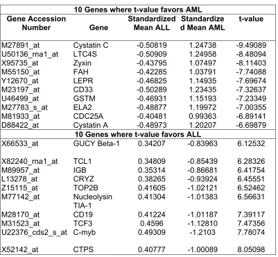
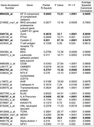
predictor genes based on the t-values and stepwise discriminant analysis, and evaluated

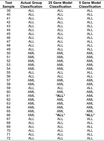
the resulting model’s performance in predicting 34 test samples by discriminant analysis.

Only two samples were not correctly predicted with 25 predictor genes we chose. We

(2)

minimum number of genes required to maintain a high level of accuracy in predicting

cancer types.

The accumulation of microarray data can help elucidate the gene regulation

mechanisms in cells. Here, we attempted to find an improved matrix description for

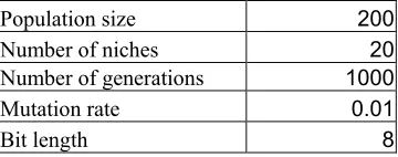
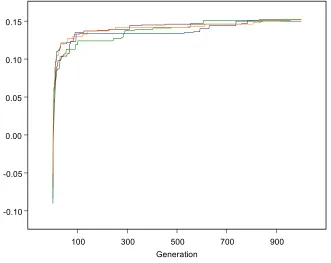
transcription factor binding site. We applied a genetic algorithm (GA) to derive matrices

that were trained from a set of true binding sequences and random sequences. Preliminary

results indicate that the matrix derived shows a higher specificity in binding site

prediction than the regular position weighted matrix (PWM) within a range of cutoff

scores. The binding site of the cell-cycle related transcription factors, E2Fs, was taken as

an example to illustrate our method. When both the GA-derived and regular matrices

were applied to scan the human gene upstream sequences, the matrix we derived gave

significant less predictions than the regular matrix, given the same false negative rate

(3)

ANALYSIS ON MICROARRAY DATA AND

DNA REGULARTORY ELEMENTS

PREDICTION

by

JUN LU

A dissertation submitted to the Graduate Faculty of

North Carolina State University

in partial fulfillment of the

requirements for the Degree of

Doctor of Philosophy

BIOINFORMATICS

Raleigh

2002

APPROVED BY:

_____________________________ _______________________________ Spencer V. Muse Sandra E. Dunn

Chair of Advisory Committee

_____________________________ _______________________________ Bruce S. Weir Gregory C. Gibson

(4)

(5)

BIOGRAPHY

LU, JUN was born on October 4, 1970 in Jiangpu, Jiangsu province, P. R. China. He

entered the Department of Biology at Nanjing University in 1988 and received his B.S. in

Biology in 1992. Following college, he worked as a research assistant in China National

Rice Research Institute (CNRRI) at Hangzhou, China. In August 1997 he came to the

United States for his graduate study at North Carolina State University (NCSU). He was

in Forest Biotechnology Group at NCSU, and later transferred to the newly established

Bioinformatics program to pursue his Ph.D. degree. During his graduate study, he also

worked as a research intern at DNA Science Laboratory, Morrisville, NC, and National

(6)

ACKNOWLEDGEMENTS

I would like to express my most sincere gratitude to Dr. Bruce Weir, and Dr.

Spencer Muse, for their support, encouragement and guidance I need to stay on track

during the graduate study. They have helped shape my research projects and provide

numerous suggestions to this dissertation.

I would like to say a special thanks to Susan Spruill, Dr. Sandra Dunn, and Dr.

Leping Li for their tremendous help on the projects, and for being mentors and friends.

Without them, this dissertation would not have happened.

Thanks also to the other committee members, Dr. Gregory Gibson, Dr.

Zhao-Bang Zeng, and my graduate representative, Dr. Brian Wiegmann for the reviewing of

this work and continuous support.

I am truly grateful to Dr. Ross Whetten and Dr. Ron Sederoff for the generous

support and mentoring when I was in their lab. Thanks are extended to many people in

the Forest Biotechnology Group for their friendship.

I would also like to express my appreciation to DNA Science Laboratory and

Biostatistics Branch at NIEHS for the generous financial support and many helpful

suggestions from Dr. Clare Eisenberg and others in the microarray discussion group at

NIEHS.

I would also like to say thanks to many good people at BRC, in particular, Debra

Hibbard, Amy Elkins, Lisa Barefoot, Dr. Sarah Hardy and fellow graduate students for

(7)

Finally, I would like to say thanks to my wife, Mingyan, for the encouragement,

endless support and love. I am grateful to her for always standing by with me during the

(8)

LIST OF TABLES

Chapter 2

1. The schematic representation of the origin of eight quadrants on a slide 59

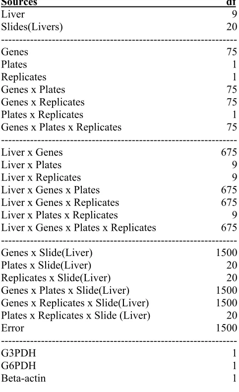
2. The full ANOVA model and the associated degree of freedoms (df) 59

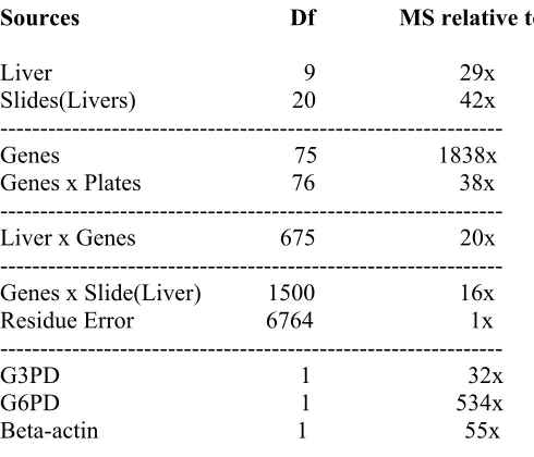
3. The ANOVA table based on the reduced model 60

4. Sources of variation from the ANOVA partition 60

Chapter 3

1. Results from T-Test 77

2. Genes obtained from Stepwise Discriminant Analysis 78

3. Classification results from discriminant analysis 80

Chapter 4

1. A set of GA parameters used 106

2. A list of experimentally confirmed E2F binding sites 108

3. Comparisons between the regular and the GA-derived matrix 110

4. A list of genes containing potential E2F binding sites with –300

(13)

LIST OF FIGURES

Chapter 2

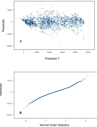
1. Observed residual plotted against predicted values and normal order

Statistics obtained from the ANOVA model fitting 61

2. Box plots of the three slides hybridized in each liver 62

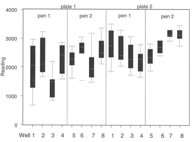
3. Box plots of the wells within each pin and plate arrangement 62

Chapter 3

1. Scatter plot means of AML and ALL for 25 genes and 5 genes used in

discriminant analysis 79

Chapter 4

1. A diagram showing the evolution based on genetic algorithm 106

2. An example of PWM based on dataset train_30 107

3. The increase of fitness scores based on 4 independent runs 107

(14)

Chapter 1 Literature Review of Microarray Technology and Data Analysis

Introduction

Understanding the mechanisms of gene regulation has been a main focus of molecular biologists for many years. The control mechanisms for gene expression in eukaryotes are complex and the regulation can occur at the chromatin DNA level, during mRNA synthesis (transcription), RNA processing, protein synthesis (translation) and after protein translation (Lewin 1997). Among these possibilities, control at the

transcription level is one of the key steps and has been studied intensively (Ptashne and Gann 1997, 1998). The amount of expressed RNA of a gene is traditionally measured by Northern blot or dot blot (Sambrook and Russell 2001). Briefly, the total RNA or mRNA samples are transferred and UV cross-linked to nylon membranes (with or without size separation). Then, a DNA fragment that represents the gene is radioactively or non-radioactively labeled and hybridized with the RNA samples on the membrane. After the hybridization and washing steps, the hybridization signal is often detected by

autoradiography. The difference on signal intensity between a control and a treatment sample indicates the differential expression of a gene. One thing should be pointed out is that the Northern blot or dot blot can only measure the expression level of one gene in each hybridization process.

(15)

driven by the advance of new technology, such as high-throughput sequencing (Venter et al 2001; Lander et al 2001), large-scale genotyping (Syvanen 2001; Cutler et al 2001) and transcription profiling (Brown and Botstein 1999; Lipshutz et al 1999). In particular, a number of techniques have been developed to measure the cellular mRNA levels on a global scale, including serial analysis of gene expression (SAGE) (Velculescu et al 1995), cDNA microarray (Schena et at 1995) and oligonucleotide chips (Lockhart et al 1996; Mcgall et al 1996). Such high-throughput methods significantly accelerate our

understanding of the complex biological process by allowing the identification of gene expression patterns from the broad assessment of gene transcription. Compared to traditional methods such as Northern or dot blots, the microarray and oligonucleotide technologies have been developed to measure the RNA transcript levels of hundreds or thousands of genes at a time. In principle, the way of measuring the RNA levels with microarrays or oligo-nucleotide chips is the same as that with Northern or dot blot. The major difference is that the positions of the probes (DNA fragments representing genes) and the targets (i.e. total RNA or mRNA samples) are reversed in microarray

(16)

In this chapter, I will first give a brief review on microarray techniques. The focus will then be on how the microarray data is analyzed, including data normalization,

identification of differentially expressed genes, and recognition of gene expression patterns

Part I: Review of microarray techniques

In general, there are two types of microarrays that are commonly used: cDNA microarrays (Schena et al 1995) and Affymetrix oligo-nucleotide chips (Lockhart et al 1996). Although the strategies of constructing the arrays (chips) are different, the basic idea is the same: the relative concentration of a target mRNAs in a given sample is measured through hybridizing a labeled RNA sample to tens of thousands probes on an array (chip). Since the cDNA arrays can be made in a lab, there is more flexibility in choosing genes for spotting on an array. In contrast, the oligo-nucleotide chips are only commercially available (from Affymetrix Inc.), the sets of genes on a chip have been pre-chosen and the DNA chips have been made for users, which is less flexible than cDNA arrays. On the other hand, preparing the cDNA arrays in labs can introduce unexpected variations and the comparison of experiments conducted in different labs can be difficult due to the different sets of genes and the protocols used.

cDNA microarrays

(17)

slides in which tens or thousands of genes (represented by DNA fragments) have been spotted with high density. After the slides are made, they can be stored for a period of time. The second stage starts from the extraction of total RNA (or mRNA) to the data collection, which is often conducted and finished within a week.

(1) Array preparation

The Source of DNA The first step is to prepare DNA for spotting. Although the synthesized oligo-nucleotides can be used, in eukaryotes, the source of DNA is often from a constructed cDNA library that contains tens and thousands of clones. Each clone includes one species of expressed DNA fragment representing one gene. The cDNA clones can be sequenced, and the single run, partial sequence of a cDNA is called an expressed sequence tag (EST). Since the amount of DNA in each clone is very small, the DNA fragment needs to be amplified, usually through polymerase chain reaction (PCR). The size of PCR amplified products generally ranges from 0.3 to 3 kilobases (Kb). Usually the PCR reactions are conducted in a high-throughput way. For example, a 96-well plate can hold 96 PCR reactions and each reaction amplifies one cDNA clone

(representing one gene). After the amplification, the quality and quantity of PCR products are checked by gel electrophoresis (Sambrook and Russell 2001). Any failure or

(18)

One important issue that needs to be addressed is gene redundancy. Ideally, the DNA fragments spotted on the glass slides should represent as many genes as possible. However, the highly expressed genes in a cell would appear more frequently than the low-abundance genes if the library clones were randomly chosen. In order to avoid such problems, the partial sequence information of the clones may be necessary to identify each clone. For instance, if a given cDNA clone has been partially sequenced, the EST sequence information in UniGene database (http://www.ncbi.nlm.nih.gov/UniGene/) can be helpful to determine whether the cDNA clone is unique on an array (Pruitt and

Maglott 2001). For human cDNAs, there is another database called Human Gene Index (http://www.tigr.org/tbd/hgi/hgi.html), in which all the human ESTs have been clustered with one cluster representing one gene (Quackenbush et al. 2000).

(19)

has strong binding on the slide surface. Also DMSO has lower evaporation rate than 3XSSC, which allows the spotting DNA to be stored for a longer period of time (Hegde et al 2000).

The DNA is spotted on coated glass slides by robots. Brown’s lab designed the original robot at Stanford University (Schena et al. 1995; Eisen and Brown 1999). Currently, a number of companies are selling such high-speed robotic systems, such as Intelligent Automation Systems (IAS) (http://www.ias.com), Genomic Solution

(http://www.genomicsolutions.com) and others. The robots array DNA samples

(dissolved in spotting solution) from 96- or 384-well microplates to slides using printing pins. One critical point for evaluating the quality of the robotic system is the consistency among these pins. The geometry of the pins greatly affects the size and the shape of spots on a slide, along with some other factors including humidity and temperature (Hegde et al. 2000; Eisen and Brown 1999). The printed DNA is bound to slide by ultraviolet (UV) cross-linking, and the slides can be stored in a dessicator at room temperature.

(2) RNA labeling, hybridization and data collection

RNA labelingThe total RNA is extracted from the treatment and control samples through standard methods (Sambrook and Rusell 2001) or using RNA extraction kits that are commercially available for instance, RNeasy kit from Qiagen

(http://www.qiagen.com), and TRIzol from Life Technology

(20)

first strand cDNA by reverse transcriptase with the oligo-dT as primers. The labeled nucleotides, such as Cy3 or Cy5 –dUTP, are added into the reaction mixtures and incorporated into the first-strand cDNA. After the labeling reactions are finished, the unincorporated Cy3 or Cy5 –dUTP needs to be removed by filter filtration or ethanol precipitation that is similar to the PCR product cleaning. Since the Cy3 and Cy5 –dUTP are light sensitive, the reactions and all the following steps should avoid light as much as possible. The final product is the first-stand cDNA labeled with Cy3 or Cy5. An equal amount of the Cy3 and Cy5 labeled products are mixed and denatured just before hybridization (Schena 1999; Eisen and Brown 1999; Hegde et al. 2000).

(21)

stringency condition refers to washing steps with solutions containing low concentration of salt (Eisen and Brown 1999; Hegde et al. 2000).

Data collection First, the confocal laser scanner is used to scan the hybridized arrays. The scanner uses a laser to excite Cy3 and Cy5 dyes and the emission signals are then recorded. Two separate TIFF images will be obtained with one from the Cy5 and the other from the Cy3 channel. Next, the two image files are further processed and the images are transferred to quantitative data through spot identification (gridding), signal, and background estimation from the pixel intensities (Schena 1999; Eisen and Brown 1999). Although a number of software packages for image processing are available, for instance ScanAlyze (http://rana.lbl.gov/EisenSoftware.htm; Eisen and Brown 1999), in many cases human intervention is necessary due to the irregularities of the spots. Both the distance of spots and the spot size need to be adjusted to cover the true spot area. Finally, the foreground and the background intensities of each spot are estimated by either the median or the mean of the pixel values within the spot ellipse (Hegdes et al 2000). Sometimes, the spot quality is evaluated based on the pixel values and listed as well (Yang et al 2000). It has been noticed that the image processing can vary

substantially from one lab to the other, which can introduce significant amount of variation into the data (Yang et al 2002; Eisen and Brown 1999; Hegde et al 2000). The final data for one hybridization experiment is often in the form of a table in which the rows list the names of genes and the columns represent the values of background

intensities, the signal intensities, and possibly the quality measurements for each spot.

(22)

The DNA chips produced from Affymetrix Inc. have been widely used as well (Lockhart et al 1996; Mcgall et al 1996). The major difference between DNA chips and cDNA arrays is that, instead of a long fragment of cDNA, 20 pairs of 25-mer

oligonucleotides represent one gene on each DNA chip. Among the 20 pairs of

oligonucleotides represented for each gene, 10 pairs are negative sets with only one base pair (in the middle) different from the corresponding positive sets that have the exact matches to the gene sequence. The DNA chip arrays are created by Affymetrix's light-directed chemical synthesis process, which combines solid-phase chemical synthesis with photolithographic fabrication techniques employed in the semiconductor industry

(http://www.affymetrix.com; Mcgall et al 1996). The detail of this process is rather technical and will not be described here. Basically, the known sequences of

(23)

Conclusion

Although microarray technology has been developed for nearly a decade, the laboratory techniques are still evolving. Many factors can affect the accurate

measurement and comparison of expression intensities in different samples, in particular, the comparisons between arrays or DNA chips. Reproducible and reliable data is

essential for further data analysis and for drawing scientific conclusions.

Part II. Review of gene expression data analysis

Currently, microarray (chip) technology has two primary types of application: (1) identifying the differently expressed genes among two or more experimental conditions and (2) finding gene expression patterns. In the first situation, the main interest is on finding genes that are up or down regulated between two or more samples (for example, between cancer and normal samples). Usually the question is answered through designed experiments, in which the sources of variation are generally under control. Identifying differentially expressed genes is simply a task of conducting hypothesis tests of whether the levels of mRNA transcripts are equal between two or more samples. Examples of this type of application include the identification of target genes of the c-Myc transcription factor (Coller et al 2000), stain and region-specific genes in mouse (Sandberg et al 2000), and genes responding to ionizing radiation (Tusher et al 2001).

(24)

variation in experiments (since they may have been conducted in different labs). The main interest is more on finding the relationships among a group of genes or samples rather than finding a specific gene. The typical examples of finding gene expression patterns include cancer sample classification (Golub et al 1999; Alon et al 1999) and identification of co-regulated gene clusters (Brazma et al 1998; Spellman et al 1998; Eisen et al 1998).

There are other types of applications on using microarray technology, such as SNP identification (Cutler et al 2001) and DNA-binding site identification (Iyer et al 2001). These areas are beyond the discussion here where the focus is on studying gene

transcription.

Data normalization

Current microarray technology is far from giving precise measures of mRNA transcript concentration, especially for those genes with low-level expression. As we discussed in Part I, a number of steps are involved in a microarray experiment, and each step could potentially introduce systematic variation into the final data. For example, variation can be introduced during the dye labeling reaction, slide preparation (for

instance, pin, slide) and slide hybridization (Kerr et al 2000; Schuchhardt et al 2000). The sources of variation can also arise from physiological and biological sampling, which have been nicely illustrated by Novak et al (2002) and Pritchard et al (2001).

(25)

Unfortunately, there is no consensus on how the data should be normalized, and the choice of the normalization methods is also depends on the experimental design of an experiment (Kerr et al 2000; Wolfinger et al 2001).

Normalization can be either conducted first as a preliminary step or integrated into the data analysis process (Yang et al 2002; Wolfinger et al 2001; Kerr et al 2000). In general, there are two types of normalization methods: global and intensity-dependent normalization. Global normalization means that the same scaling factor will be applied to every gene on a slide, regardless of the intensity values of genes. Examples of global normalization include ANOVA-based method (Kerr et al 2000), the normalization by linear regression (Golub et al 1999), and other mean or median based normalization methods (Spellman et al 1998; Quackenbush 2001). In contrast, intensity-dependent (or local) normalization takes the difference of individual genes into account, and assumes that the intensities are non-linear. Local normalization is usually carried out through local regression, such as LOWESS (Locally Weighted Scatterplot Smoothing) regression (Yang et al 2002).

(26)

labeled hybridization products (Schuchhardt et al 2000; Tseng et al 2001). Such systematic variation has to be accounted for in the following data analysis. Currently, three normalization methods are widely used for data generated from a single slide hybridization. The first method is based on the total intensity values of two samples. The method depends on the assumptions that the total intensities from each labeled samples should be equal, and genes that are up-regulated are balanced out by the down-regulated genes in the same array. A rescaling factor can be calculated by assuming either equal median or equal mean between two samples (Cy3 and Cy5 channels). This factor is then assigned to each gene on the array (a strategy of global normalization). The second normalization method commonly used is based on regression. Again, the assumption is also made that the slope of the regression line between two samples should be one if there is no systematic variation involved. The basic steps include finding the least-square regression line on the scatter-plot of Cy5 versus Cy3 channel, and the slope is used to rescale the intensity values. In some cases, non-linear intensity is assumed and a local regression is conducted, such as LOWESS (Yang et al 2002). Another way of

normalizing the data is described by Chen (1997). They derived a probability density function for the ratio of two channel intensities of the housekeeping genes on the array, and use that to iteratively adjust the mean expression ratio to one. The density of the ratio can also used to construct confidence intervals and to identify the differentially expressed genes (Chen et al 1997).

(27)

estimates for statistical inferences (Kerr et al 2000). After normalization steps, the data are either ratio values (log ratios) or intensity values, and further analysis such as classification is based on these normalized data matrices.

Identifying differentially expressed genes

A common application of microarrays is to identify genes that are differentially expressed between two samples. The ratio-based approaches have been widely used for two-dye cDNA microarrays (Chen et al 1997; Chu et al 1998). The expression ratio is the normalized value of a treatment sample divided by the normalized value of a control sample, and is calculated for every individual gene on a slide. The base 2 logarithm of the ratio is often used. Typically the genes that show log-ratio greater than 1 (two-fold

increase or decrease of the gene expression) are considered as differentially expressed. The advantage of calculating the log-ratio of expression value is easy to understand for biologists since 2-fold change has a log-ratio of 1. However, use of the ratio statistic has been drawn criticism since the ratio totally ignores the absolute values of the expression levels and the variation in the data (Wittes and Friedman 1999; Wolfinger et al 2001). The absolute value matters because it has been well known that low-intensity values often associate with high variation. Thus, the low intensity value can give high ratio values, however, those values are most likely unreliable (Tanaka et al 2000).

(28)

they found is that, even for the simple design, a large amount of variation within a gene was detected. They recommended a minimum of three replicates for this simple design. Another example is given by Pritchard et al (2001), in which they addressed the

biological variation problem. By using analysis of variance (ANOVA) techniques, they found that 0.8, 1.9, and 3.3 percent of genes were normally variable in the mouse liver, testis and kidney, respectively. Among the variable genes, the stress-related, immune-modulated, and hormone-controlled genes were highly represented. Their experiment demonstrates that the biological variation could be introduced easily by handling the mouse differently and some genes often show variability without any relation to the biological difference of interests. Without replication, there is no way to distinguish such variation from the true treatment differences. A recent study by Tanaka et al (2000) gave another example of the danger of strictly using the fold-change to evaluate the change of the gene expression.

There are at least two purposes for conducting the replicated experiments. One is to accurately estimate the systematic variation, which is necessary for normalization. Another reason of having replicates is to estimate the random error, which can then be used to conduct statistical inference on changes of gene expression (Kerr and Churchill 2001). For replicated microarray experiments, the task of identifying differentially

(29)

parameters are estimated based on all the data, rather than a piece of information. Instead of using log ratios, the model was derived from the logs of original intensity values, which avoided the drawback of using ratios and preserved the data properties necessary for an additive effect model. Since the ANOVA model is tightly linked to the issue of experimental design, the authors also illustrated how different designs affected the parameter estimation. Finally they applied a resampling-based method (bootstrap) to derive the confidence intervals for estimates of differential expression of each gene, as opposed to assuming normal distributions for the residual errors (Kerr et al 2000; Kerr and Churchill 2001). Wolfinger et al (2001) further extended the ANOVA model by assuming some effects to be random, such as the array effect. The mixed model can provide broader inference on the gene expression. Also, the normalization process was conducted separately from the gene identification step. Briefly, they constructed two interconnected ANOVA models, the ‘normalization model’ and the ‘gene model’. The normalization models are fit to the data first (to normalize the data) and the residuals derived were the input data for the gene models. Advantage is that separate gene models allow inference to be made with individual error estimates for each gene (heterogeneity), which is consistent with the observation that genes with low intensity values display high intra-gene variability.

(30)

A unique feature of microarray data is that usually there are very few replicates for each gene in a experimental sample but a large number of genes on the array, which makes the traditional t-test or rank-based nonparametric tests not effective. Efforts have been made to draw statistical inferences based on the distributions of quantities including the whole data on the array. For example, Pan et al (2001) proposed to estimate the distributions of two t-statistic-type scores using normal mixture models. The differentially- expressed genes were identified through the comparison of two

distributions (one from each channel) by likelihood ratio tests. Baldi et al (2001) applied a Bayesian approach to make statistical inference on gene expression changes. Other methods for identifying differentially expressed genes directly model the ratio values (log-ratios) (Chen et al 1997; Newton et al 2001).

Finding gene expression patterns

Given a normalized gene expression matrix, one broad area of the application of microarray data is to identify the gene expression patterns existing in a large amount of data (Eisen et al 1998; Alon et al 1999; Brazma and Vilo 2000). Here the patterns simply refer to a number of common features shared either by a group of genes or a group of samples. The methods used in finding patterns can be divided into two categories:

unsupervised learning and supervised learning. We call an unsupervised learning method if no expert knowledge is involved in the data learning process. Examples of

unsupervised methods include hierarchical clustering (Eisen et al 1998) and

(31)

training data set will be constructed, including one or more classes of known functionally related genes (positive set) and one or more groups of genes not belonging to those classes. Supervised methods then learn to discriminate between the known group members and non-group members of a given class based on the gene expression data (Brown et al 2000). We discuss some of the methods commonly used in each category.

Unsupervised learning

The typical example of unsupervised learning is sample (gene) classification. Most work has focused on grouping genes into clusters based on expression data. The motivation of conducting cluster analysis is that genes in a particular pathway or involved in a specific process may be co-regulated and show similar expression patterns.

Various methods have been applied in cluster construction based on gene

expression data. The most popular one is hierarchical clustering (Eisen et al 1998), which is described as follows. We define each gene by an expression vector, and the values in the vector are the expression measurements under different experiment conditions. The measurements can be the exact values or the relative ratios to a reference sample. The distance between two gene-expression vectors reflects how similar the two genes are. There are various methods for measuring distance, and the widely used one is Euclidean distance. Let D represents the distance between gene X and Y, the Euclidean distance is calculated by the following equation:

2 1

( )

n

i i

i

D x

=

∑

−y

where xi and yi are the expression values of gene X and Y at condition i respectively.

(32)

algorithms, including single-linkage algorithm, complete-linkage clustering, average-linkage clustering and others (Quackenbush 2001). For example, the average-average-linkage clustering algorithm finds the closest two genes first from a pairwise distance matrix of all n gene vectors. A node is created joining these two genes, and the node is then represented by a new expression vector calculated by the average of the expression vectors of two genes. The pair-wise distance matrix is then calculated again among n-1

gene (node) vectors included, and the vectors with lowest distance are joined and form a new node. This process is carried out iteratively until all gene-vectors are in one cluster.

Hierarchical clustering is simple to implement and the results can be easily visualized. The major problem with cluster analysis is that phylogenetic-type cluster structures do not reflect the actual relations among genes in biological systems. A difficulty would arise if one gene participates in more than one regulatory or metabolic pathways. Another problem with this method is that once an incorrect assignment is made at an early stage, there is no way to correct it later on. Other clustering algorithms include k-means clustering (Tavazoie et al 1999) and self-organizing maps (Tamayo et al 1999). Both methods rely on other sources of information to pre-determine the number of clusters in the available data, which may not be realistic in situations where we know nothing about the whole structures of the data.

(33)

added into the correlation in order to capture the negative relations between genes (features). 2 2 ˆ ( ) r r r abs r = 2

r is representing the Pearson correlation coefficient. High represents the hypothesis of a biological relation. Instead of grouping all genes into one cluster by hierarchical clustering, a relevance network only retains the significant relationships among features

by threshholding. The cutoff value is empirically determined by repeated random

permutation study. For each feature pair, the measurement is permuted 100 times, and is calculated for each permuted set. In Butte’s paper, a threshold value 0.8 is chosen

because no permutated data set can produce the absolute value greater than 0.8 (so the

p-value is less than 0.01 in this case). Groups of features with an value greater than the threshold will aggregate and form the relevance network. The threshold value can be adjusted to include biological meaningful relations in the relevance network. In a relevance network, a gene can be directly or indirectly connected to several genes or other phenotypic measurements, which is an obvious advantage over tree-type clustering methods. The cross-connected networks represent not only pair-wise but also aggregated associations, which are the most trustable relationships between features. The example given in the paper successfully clustered the base line expression measurements in cancer cell lines and measurements of anticancer agent susceptibility in the same set of cell lines. 2 ˆ r 2 2 ˆ r 2 ˆ r ˆ r 2 ˆ r

(34)

associations if we choose a high cutoff value, and we may produce many false-positive hypotheses if we relax that criterion.

Gene or sample classification has been the most popular method to search for possible expression patterns in the data. A great deal of effort was made on deriving the best classification method. However, little attention has been paid to the reliability of the clustering results, given the inherent noise associated with microarray data. Kerr and Churchill (2001) addressed this question by using bootstrapping techniques to evaluate stability of results from a cluster analysis. Basically, they assume that the “true” clustering C can only be obtained if the true expression differences r are known. In practice, the true expression differences can only be estimated from observed data, .

Thus, the true clustering C can only be estimated by . This means the results from any clustering methods have variation if the error of estimation is considered. In the paper, they applied the bootstrapping method to create a collection of bootstrapping clusters

{C*}, in addition to the original cluster C based on the estimates of relative gene expression . A gene was claimed “95% stable” in a cluster (profile) if it occurs in at least 95% of the bootstrap clusters. The final results they received were the number of genes in each profile having a pre-defined bootstrap stability (for instance 95% stability). Obviously, the number of genes in a cluster would be smaller with 95% stability than with 80% stability (Kerr and Churchill 2001).

ˆ

r

ˆ C

ˆ

r

(35)

the t-statistic. They found that the genes showing differential expression were grouped separately from the genes with no expression changes based on the assumed model. Another advantage of using model-based clustering is that it can calculate the posterior probability of an observation belonging to a cluster (Pan et al 2002).

Supervised learning

As has been mentioned, the supervised learning methods take prior knowledge on samples (genes) into account. Theyt attempt to derive models from a set of training samples, and then use the model to predict a new sample (or gene). Obviously, the main part is to derive a model that can discriminate between the known group and non-group members of a given class based on the gene expression data. Brown et al (2000)

introduced a supervised method, support vector machine (SVM), which has been widely used in pattern recognition in computer science (Vapnik 1998). SVM uses the biological information in the training data to determine the important characteristics in each class, and then use this knowledge to determine whether a new gene should be classified into a specific class (Brown et al 2000).

For a two-class classification problem, assume we have a set of gene expression vectors xi (i = 1, 2, …, n) measured at p experimental conditions. Also assume there

(36)

into a higher dimension feature space. Then, any training data set can be separable if we can choose an appropriate feature space with sufficient dimensionality. SVM takes this approach by mapping the input vectors into a high dimensional feature space and constructs an Optimal Separating Hyperplane (OSH). OSH maximizes the margin, the distance between the hyperplane and the nearest data points of each class in the feature space. The specification of a SVM requires two parameters: the kernel function which defines an inner product of two expression vectors in the feature space, and a

regularization parameter which controls the trade off between margin and

misclassification error. Letting xi and xj represent two expression vectors, two typical

kernel functions are:

( , ) ( 1)d

i j i j

K x x = x x• + ,

2

( , ) exp(_i _j _i _j )

K x x = −γ &x −x & .

The first one is the polynomial kernel function of degree d, and the second one is the radical basic function (RBF) kernel with parameter γ .

Brown et al (2000) construct the SVMs to recognize six functional classes:

(37)

RBF SVM and third-order SVM generally perform better than other methods. An interesting comparison is also conducted between higher-order SVM and hierarchical clustering methods. Among known 121 ribosome genes, SVM correctly identifies 118 genes with 7 false positives, and by hierarchical clustering method, the ribosome cluster found 112 genes with 14 false positives. The supervised learning is considered promising since it directly combines the known knowledge with the expression data. The limitation of SVM is that some biological classes may not be recognizable based on transcription data alone.

Besides the SVM, there are other classical supervised methods, including the k

nearest-neighbor (KNN) classifier, linear or quadratic discriminant analysis, and

classification and regression trees (CART) (Webb 1998). In addition, results have shown that combining predictors from perturbed versions of the leaning set could increase the prediction accuracy (Breiman 1998).

One of the most successful applications of pattern recognition approaches using expression data is on the classification and prediction of tumor types or subtypes. Alizadeh et al (2000) applied DNA microarray expression data to distinguish the subtypes of diffuse large B-cell lymphoma (DLBCL). Their results also show that the molecular classification of tumors on the basis of gene expression can identify previously undetected and clinically significant subtypes of cancer. The SVM has been applied to multiclass cancer classification problem (Ramaswamy et al 2001). A total of 218 tumor samples spanning 14 common tumor types are classified by SVM algorithm based on expression data, and the overall accuracy is 78%.

(38)

Prediction of gene regulatory elements

Gene (or sample) classification using either supervised or unsupervised methods is only the first step in expression data analysis. The final goal of conducting

transcription profiling is to elucidate the functional roles of the respective genes and to further understand the underlying biological processes. An immediate next step of microarray data analysis is to seek possible regulatory elements in the genomic

sequences. A number of studies on predicting gene regulatory elements have been carried out in yeast (Brazma et al 1998; Hughes et al 2000; Tavazoie et al 1999). An assumption is often made that genes with similar expression patterns may share a common regulatory mechanism, such as transcription factor-binding sites. Therefore, the main goal is to find motifs (DNA elements) that are over-represented in a group of genes.

One area of study is to identify the potential regulatory elements in a group of functionally related genes. Most studies on finding DNA motifs were conducted in yeast, since the yeast promoter region is relatively well defined and close to the coding regions. For instance, Vilo et al (2000) used a public data set to carry out cluster analysis of 6221 genes based on the measurements from 80 conditions. For each cluster, the 600 bp upstream sequences were extracted for each gene, and all substrings with variable length were searched and assigned a probability score according to binomial distribution if it appeared in more than ten sequences. A total of 1498 substrings were selected based on a significance threshold determined by a randomization test. The substrings were further grouped into 62 clusters of patterns, and were searched against the known transcription factor in the yeast database SCPD (The Promoter Database of Saccharomyces

(39)

transcription factor binding sites. The remaining patterns may be either the false positives or ones that have not been identified yet, which could be new targets for further

experimental study (Brazma 1998). A similar example was given by van Helden et al (1998) in which they also searched for over-represented oligonucleotides in a group of sequences. Both methods conducted an exhaustive search for sub-strings that meet the defined level of statistical significance.

Another strategy for discovering the DNA motifs is through the Gibbs sampling algorithm, which was previously used to find motifs in protein sequences (Lawrence 1993, Neuwald et 1995). Gibbs sampling is one of the Monte Carlo Markov Chain techniques for sampling from posterior distributions. For the case of searching DNA motifs in a group of sequences, the goal of Gibbs sampling is to find the starting location of a motif within each sequence and estimate the residue frequencies at each position of the motif. There are two versions of Gibbs sampler: site sampler and motif sampler. The Site sampler considers the simple case, where each motif is assumed to occur in every sequence and only once. The motif sampler is more general by allowing 0 or more motifs in each sequence. Given a group of sequences and the length of motif, three steps are involved in Gibbs sampling (An example of site sampler).

Notation:

S: a group of sequences (known)

W: the width of a motif (known). The motif is assumed to be ungapped.

ci,j: observed counts of residue j at position i of a motif. i ranges from 1 to W, and j

(40)

qi,j: the frequency of the residue j at position i of a motif. q0,j represents the

background frequencies of the four residues.

ak: Vector of starting positions of a motif in sequences S. k ranges from 1 to N, where

N is the number of sequences. (1) Initialization

The site sampler is initialized by randomly assigning a starting location of the motif within each sequence, and the location of starting points is recorded as a vector ak. The frequencies of residues at each position within a motif, along with

the background frequencies (sequences outside the motif), can be calculated. Usually pseudocounts for each residue are needed to avoid problems with zero probability.

(2) Predictive update step

The first step is to select one sequence (among N sequences) and place the motif sequence (with length of W) within the selected sequence in the background. The motif frequency matrix is updated based on the alignment (with N-1 sequences), along with the background residue frequencies.

(3) Sampling step

The sampling step is to find the starting position of the motif in the sequence that has been selected in step 2. All possible starting positions will be considered. One way of drawing samples is as follows. For a fragment X (with length W) from a given start point, a weight Ax is calculated based on the likelihood ratio, in which

(41)

sampling, the starting position will be chosen with the probability proportional to the weight. The positions with higher weights will be more likely to be selected than the positions with lower weights. Once the iterative predictive update and sampling steps have been conducted for all of the sequences, a probable

alignment will appear and an associated F score will be calculated as well, where

F is given by the formula

, ,

1 1 0,

log

W J

i j i j

i j j

q

F C

q

= =

=

∑∑

The predictive update and sampling steps will be conducted again on each sequence of S, given the data and the start points that have been chosen. The whole process will be run iteratively as a Markov chain. As the number of iteration is large

enough, the joint distribution of ( will converge to joint posterior

distribution

( ) ( ) ( ) 1 , 2 ,..., )

i i i

N

a a a

1, 2,

( ..., _N| )

f a a a S .

Gibbs sampling is a heuristic and not an exhaustive search, so the method will give an optimal result but may not be the best. The method is very sensitive to the subtle DNA patterns existing in a group of sequences, but requires the knowledge on the length of a motif. A program AlignACE was specifically written for scanning multiple motifs in a given set of DNA sequences by using a Gibbs sampling strategy with some

(42)

Conclusions

Appropriate analysis of microrray data is critical to draw scientific conclusions. The first data normalization step can have significant influence on downstream analysis. The identification of differentially expressed genes can provide clues on the function of genes in a particular biological process. The finding of gene expression patterns allows one to predict gene function, classify normal and disease samples for future diagnosis, and to help elucidate the mechanisms of gene transcription.

Outline of the present study

The remainder of this dissertation is organized into three chapters. The first chapter addresses the variation problem existing in a typical micorarray experiment. The objective is to identify sources of variation and provide knowledge for future experiment design. It is titled “Addressing the sources of variation in gene expression data”. In the second chapter, we demonstrate that molecular cancer classification could be approached by discriminant analysis combined with T-statistics, and the prediction result is better than that published by Golub et al (1999). In the fourth chapter, we present the

preliminary results on improving matrix representations of transcription factor binding sites, which is titled “Toward improved matrix description of E2F binding sites”.

References

(43)

D. D., Armitage J. O., Warnke R., Staudt L. M., et al. (2000) Distinct types of diffuse large B-cell lymphoma identified by gene expression profiling. Nature. 403(6769):503-11.

Alon U., Barkai N., Notterman D. A., Gish K., Ybarra S., Mack D., Levine A. J.. (1999) Broad patterns of gene expression revealed by clustering analysis of tumor and normal colon tissues probed by oligonucleotide arrays. Proc Natl Acad Sci U S A. 96(12):6745-50.

Baldi P., Long A. D.. (2001) A Bayesian framework for the analysis of microarray expression data: regularized t -test and statistical inferences of gene changes. Bioinformatics. 17(6):509-19.

Brazma A., Jonassen I., Vilo J., Ukkonen E.. (1998) Predicting gene regulatory elements in silico on a genomic scale. Genome Res. 8(11):1202-15.

Brazma A., Vilo J.. (2000) Gene expression data analysis. FEBS Lett. 480(1):17-24.

Breiman, L.. (1998) Arcing classifiers. The Annals of Statistics. 26:801-824.

(44)

Brown P. O., Botstein D.. (1999) Exploring the new world of the genome with DNA microarrays. Nat Genet. 21(1 Suppl):33-7.

Butte A. J., Tamayo P., Slonim D., Golub T. R., Kohane I. S.. (2000) Discovering functional relationships between RNA expression and chemotherapeutic susceptibility using relevance networks. Proc Natl Acad Sci U S A. 97(22):12182-6.

Chen Y., Dougherty E. R., and Bitter M. L.. (1997) Ratio-based decisions and the quantitative analysis of cDNA microarray images. J. Biomed. Optics 2, 364-374.

Chu S., DeRisi J., Eisen M., Mulholland J., Botstein D., Brown P. O., Herskowitz I.. (1998) The transcriptional program of sporulation in budding yeast. Science.

282(5389):699-705.

Coller H. A., Grandori C., Tamayo P., Colbert T., Lander E. S., Eisenman R. N., Golub T. R.. (2000) Expression analysis with oligonucleotide microarrays reveals that MYC regulates genes involved in growth, cell cycle, signaling, and adhesion. Proc Natl Acad Sci U S A. 97(7):3260-5.

(45)

High-throughput variation detection and genotyping using microarrays. Genome Res. 11(11):1913-25.

Eisen M. B., Spellman P. T., Brown P. O., Botstein D.. (1998) Cluster analysis and display of genome-wide expression patterns. Proc Natl Acad Sci U S A. 95(25):14863-8.

Eisen M. B., Brown P. O.. (1999) DNA arrays for analysis of gene expression. Methods Enzymol. 303:179-205.

Fraley C., Raftery A. E.. (1998) How many clusters? Which clustering methods? Answers via model-based cluster analysis. Computer J, 41:578-588.

Golub T. R., Slonim D. K., Tamayo P., Huard C., Gaasenbeek M., Mesirov J. P., Coller H., Loh M. L., Downing J. R., Caligiuri M. A., Bloomfield C. D., Lander E. S.. (1999) Molecular classification of cancer: class discovery and class prediction by gene

expression monitoring. Science. 286(5439):531-7.

GuhaThakurta D., Stormo G. D.. (2001) Identifying target sites for cooperatively binding factors. Bioinformatics. 17(7):608-21.

Hegde P., Qi R., Abernathy K., Gay C., Dharap S., Gaspard R., Hughes J. E., Snesrud E., Lee N., Quackenbush J.. (2000) A concise guide to cDNA microarray analysis.

(46)

Hughes J. D., Estep P. W., Tavazoie S., Church G. M.. (2000) Computational

identification of cis-regulatory elements associated with groups of functionally related genes in Saccharomyces cerevisiae. J Mol Biol. 296(5):1205-14.

Ideker T., Thorsson V., Siegel A. F., Hood L. E.. (2000) Testing for differentially-expressed genes by maximum-likelihood analysis of microarray data. J Comput Biol. 7(6):805-17.

Iyer V. R., Horak C. E., Scafe C. S., Botstein D., Snyder M., Brown P. O.. (2001)

Genomic binding sites of the yeast cell-cycle transcription factors SBF and MBF. Nature. 409(6819):533-8.

Kerr M. K., Martin M., Churchill G. A.. (2000) Analysis of variance for gene expression microarray data. J Comput Biol. 7(6):819-37.

Kerr M. K., Churchill G. A.. (2001) Bootstrapping cluster analysis: assessing the reliability of conclusions from microarray experiments. Proc Natl Acad Sci U S A. 98(16):8961-5.

(47)

Lander E. S. et al.. (2001) Initial sequencing and analysis of the human genome. Nature. 409(6822):860-921.

Lee M. T., Kuo F. C., Whitmore G. A., Sklar J.. (2000) Importance of replication in microarray gene expression studies: statistical methods and evidence from repetitive cDNA hybridizations. Proc Natl Acad Sci U S A. 97(18):9834-9.

Lewin B.. (1997) GENES VI. Oxford University Press, New York, NY.

Li C., Wong W. H.. (2001) Model-based analysis of oligonucleotide arrays: expression index computation and outlier detection. Proc Natl Acad Sci U S A. 98(1):31-6.

Lipshutz R. J., Fodor S. P., Gingeras T. R., Lockhart D. J.. (1999) High density synthetic oligonucleotide arrays. Nat Genet. 21(1 Suppl):20-4.

Lockhart D. J., Dong H., Byrne M. C., Follettie M. T., Gallo M. V., Chee M. S., Mittmann M., Wang C., Kobayashi M., Horton H., Brown E. L.. (1996) Expression monitoring by hybridization to high-density oligonucleotide arrays. Nat Biotechnol. 14(13):1675-80.

McGall G., Labadie J., Brock P., Wallraff G., Nguyen T., Hinsberg W.. (1996) Light-directed synthesis of high-density oligonucleotide arrays using semiconductor

(48)

Neuwald A. F., Liu J. S., Lawrence C. E.. (1995) Gibbs motif sampling: detection of bacterial outer membrane protein repeats. Protein Sci. 4(8):1618-32.

Newton M. A., Kendziorski C. M., Richmond C. S., Blattner F. R., Tsui K. W.. (2001) On differential variability of expression ratios: improving statistical inference about gene expression changes from microarray data. J Comput Biol. 8(1):37-52.

Novak J. P., Sladek R., Hudson T. J.. (2002) Characterization of variability in large-scale gene expression data: implications for study design. Genomics. 79(1):104-13.

Pan W., Lin J., Le C.. (2001) A mixture model approach to detecting differentially expressed genes with microarray data. Technical Report 2001-011, Division of Biostatistics, University of Minnesota, 2001. http://www.biostat.umn.edu/cgi-bin/rrs?print+2001.

Pan W., Lin J., Le C. T.. (2002) Model-based cluster analysis of microarray gene-expression data. Genome Biol. 3(2):RESEARCH0009.

(49)

Pruitt K. D., Maglott D. R.. (2001) RefSeq and LocusLink: NCBI gene-centered resources. Nucleic Acids Res. 29(1):137-40.

Ptashne M., Gann A.. (1997) Transcriptional activation by recruitment. Nature. 386(6625):569-77.

Ptashne M., Gann A.. (1998) Imposing specificity by localization: mechanism and evolvability. Curr Biol. 8(24):R897.

Quackenbush J., Liang F., Holt I., Pertea G., Upton J.. (2000) The TIGR gene indices: reconstruction and representation of expressed gene sequences. Nucleic Acids Res. 28(1):141-5.

Quackenbush J.. (2001) Computational analysis of microarray data. Nat Rev Genet. 2(6):418-27.

Ramaswamy S., Tamayo P., Rifkin R., Mukherjee S., Yeang C. H., Angelo M., Ladd C., Reich M., Latulippe E., Mesirov J. P., Poggio T., Gerald W., Loda M., Lander E. S., Golub T. R.. (2001) Multiclass cancer diagnosis using tumor gene expression signatures. Proc Natl Acad Sci U S A. 98(26):15149-54.

(50)

Sandberg R., Yasuda R., Pankratz D. G., Carter T. A., Del Rio J. A., Wodicka L., Mayford M., Lockhart D. J., Barlow C.. (2000) Regional and strain-specific gene expression mapping in the adult mouse brain. Proc Natl Acad Sci U S A. 97(20):11038-43.

Schadt E. E., Li C., Su C., Wong W. H.. (2000) Analyzing high-density oligonucleotide gene expression array data. J Cell Biochem. 80(2):192-202.

Schuchhardt J., Beule D., Malik A., Wolski E., Eickhoff H., Lehrach H., Herzel H.. (2000) Normalization strategies for cDNA microarrays. Nucleic Acids Res. 28(10):E47.

Shalon D., Smith S. J., Brown P. O.. (1996) A DNA microarray system for analyzing complex DNA samples using two-color fluorescent probe hybridization. Genome Res. 6(7):639-45.

Schena M., Shalon D., Davis R. W., Brown P. O.. (1995) Quantitative monitoring of gene expression patterns with a complementary DNA microarray. Science. 270(5235):467-70.

(51)

Spellman P. T., Sherlock G., Zhang M. Q., Iyer V. R., Anders K., Eisen M. B., Brown P. O., Botstein D., Futcher B.. (1998) Comprehensive identification of cell cycle-regulated genes of the yeast Saccharomyces cerevisiae by microarray hybridization. Mol Biol Cell. 9(12):3273-97.

Syvanen A. C.. (2001) Accessing genetic variation: genotyping single nucleotide polymorphisms. Nat Rev Genet. 2(12):930-42.

Tamayo P., Slonim D., Mesirov J., Zhu Q., Kitareewan S., Dmitrovsky E., Lander E. S., Golub T. R.. (1999) Interpreting patterns of gene expression with self-organizing maps: methods and application to hematopoietic differentiation. Proc Natl Acad Sci U S A. 96(6):2907-12.

Tanaka T. S., Jaradat S. A., Lim M. K., Kargul G. J., Wang X., Grahovac M. J., Pantano S., Sano Y., Piao Y., Nagaraja R., Doi H., Wood W. H.,3rd, Becker K. G., Ko M. S.. (2000) Genome-wide expression profiling of mid-gestation placenta and embryo using a 15,000 mouse developmental cDNA microarray. Proc Natl Acad Sci U S A. 97(16):9127-32.

(52)

Tseng G. C., Oh M. K., Rohlin L., Liao J. C., Wong W. H.. (2001) Issues in cDNA microarray analysis: quality filtering, channel normalization, models of variations and assessment of gene effects. Nucleic Acids Res. 29(12):2549-57.

Tusher V. G., Tibshirani R., Chu G.. (2001) Significance analysis of microarrays applied to the ionizing radiation response. Proc Natl Acad Sci U S A. 98(9):5116-21.

van Helden J., Andre B., Collado-Vides J.. (1998) Extracting regulatory sites from the upstream region of yeast genes by computational analysis of oligonucleotide frequencies. J Mol Biol. 281(5):827-42.

Vapnik, V. (1998) Statistical Learning Theory Wiley, New York, NY.

Velculescu V. E., Zhang L., Vogelstein B., Kinzler K. W.. (1995) Serial analysis of gene expression. Science. 270(5235):484-7.

Venter J. C. et al.. (2001) The sequence of the human genome. Science. 291(5507): 1304-51.

(53)

Webb A. R.. (1998) Statistical pattern recognition. Oxford University Press, New York, NY.

Wittes J., Friedman H. P.. (1999) Searching for evidence of altered gene expression: a comment on statistical analysis of microarray data. J Natl Cancer Inst. 91(5):400-1.

Wodicka L., Dong H., Mittmann M., Ho M. H., Lockhart D. J.. (1997) Genome-wide expression monitoring in Saccharomyces cerevisiae. Nat Biotechnol. 15(13):1359-67.

Wolfinger R. D., Gibson G., Wolfinger E. D., Bennett L., Hamadeh H., Bushel P., Afshari C., Paules R. S.. (2001) Assessing gene significance from cDNA microarray expression data via mixed models. J Comput Biol. 8(6):625-37.

Yang Y. H., Buckley M. J., Dudoit S., Speed T. P.. (2000) Comparison of methods for image analysis on cDNA microarray data.

http://stat-www.berkeley.edu/users/terry/zarray/Html/papersindex.html .

Yang Y. H., Dudoit S., Luu P., Lin D. M., Peng V., Ngai J., Speed T. P.. (2002)

(54)

(55)

Chapter 2 Assessing Sources of Variation in Gene Expression Data

Abstract

Analyzing the sources and quantities of variation is the basis for data normalization, for statistical inferences about changes of gene expression, and for

downstream pattern recognition. Although microarray technology has been routinely used in genomic research, Rigorous studies on variation that is intrinsic to microarray

experiments are still lacking. In this chapter, we address the variation problem by validating and evaluating the quality of data from an intensively replicated experiment. Analysis of variance (ANOVA) techniques have been applied to partition and quantify several sources of variation likely to be present in a typical cDNA microarray

experiment. The results show that significant amounts of variation can be attributed to slide, plate and pin differences. Replication of the experiment is absolutely necessary, especially at slide level. We discuss the origin of these sources of variation and provide suggestions for how to minimize or avoid them when designing a microarray experiment.

Introduction

The advent of microarray technology has significantly increased the

(56)

Although the technology has been rapidly developed and applied in answering many biological questions, the appropriate analysis of the microarray data is still evolving (Chen et al 1997; Efron and Tibshirani 2000; Baldi and Long 2001). The difficulties arise from the large dimension of the data (because of multiple genes and experimental

conditions measured) and the inherent variation existing in a microarray experiment. For example, the hundreds or thousands of genes on an array can lead to multiple testing problems if the differentially expressed genes need to be identified (Quackenbush 2001;Dudoit et al 2002). Also the variation in the data is directly connected to data normalization, which can have profound influence on the downstream analysis of array data, such as classification and DNA regulatory element identification (Wittes and Friedman 1999; Kerr and Churchill 2001).

(57)

Because of a series of steps involved in a microarray experiment, systematic variation can be easily introduced into the final data. The possible sources of variation can be due to probe, target and array preparation, hybridization, background and

overshining effects (Schuchhardt et al 2000). For example, dye effects have been shown to be significant in several studies (Kerr and Churchill 2000; Wolfinger et al 2001). Loos et al (2001) measured spot-to-spot variability within a slide and between slides with the cDNAs from the same labeling reactions. They found that their experiments were highly reproducible with spot-to-spot variability 3.8% within a slide and 5.0% between slides. Another example was given by Yang et al (2002), in which pin effects and slide effects have been addressed and integrated into the data normalization procedure. Other reported sources of variation include variability in RNA isolation, tissue-to-tissue variability, and within-tissue heterogeneity (Siedow 2001). For experiments where the sources of variation are known, several normalization methods can be taken to exclude such systematic variation from the raw data (see Chapter 1).

(58)

major sources of variation in a pre-designed experiment. ANOVA techniques were used to partition the total variation in the data and quantify the variation contributed by each factor. In an ANOVA framework, one uses the data to estimate both the relative gene expression and the magnitude of variation. Finally, based on the results obtained from ANOVA, we provide suggestions to better control for noise through changes in techniques or considerations in future experimental design.

Materials and Methods

Microarray experiments

Microarrays were prepared by spotting human genes on glass slides with a robot. A total of 79 genes were spotted in each slide, and the genes selected were often related to drug metabolism. Each gene was represented by a 50-mer oligo-nucleotide purchased from BD Biosciences Clontech (http://www.clotech.com). Also, two plates of DNA of the same set of genes were used for spotting, with 79 genes on each plate. Each gene occupied one well on each plate except for three genes, glucose-6 phosphate

(59)

was shown in the diagram (Table 1). It should be noticed that about half of the genes were spotted only by pin 1, and the other half spotted by pin 2.

Hybridization samples were prepared as follows: the total RNA was extracted separately from 10 cadaverous livers that were suitable for donor transplantation. Ten liver samples were from donors with a range of ages (15-53 years old) and ethnic background (5 Caucasians, 2 African Americans, 2 Hispanics and 1 Asian). The liver RNA samples were reverse-transcribed to cDNA and labeled with Cy-3 d-CTP, then hybridized with 3 slides for each liver sample. Only one dye was used in this experiment.

Data preparation and analysis

The final data were collected as raw readings as well as the background values. Some spots were treated as missing because of low quality signals. The raw intensities were corrected for background noise by subtraction. Subtracted values less than zero were set to zero. No efforts were made to remove outliers. All computations for the data analysis were carried using SAS software (SAS Institute, Cary, NC).

Results

The analysis of variance (ANOVA) models

(60)

Yijklm = Li + S(L)ij + Gk + Pl + Rm + G*Pkl + G*Rkm + P*Rlm + L*Gik + L*Pil + L*Rim +

L*G*Rikm + L*G*Pikl + L*P*Rilm + L*G*P*Riklm + G*S(L)ijk + P*S(L)ijl +

R*S(L)ijm + G*P*S(L)ijkl+ G*R*S(L)ijkm+ P*R*S(L)ijlm + G3PD + G6PD +

Beta_actin + Eijklm

where L represents liver (i=1, 2…10), S represents slide (j=1,2,3), G represents gene (k = 1, 2, …, 76), P represents plate (l=1, 2), R represents replicate (m = 1, 2), E represents residual error and Y represents background adjusted intensity reading. All model terms, except for E were treated as fixed effects. In addition, three housekeeping genes, G3PD, G6PD, and beta-actin, were added as covariates into the model. All effects with their degrees of freedom in the full model are listed in Table 2. In this study we were interested in identifying factors that had large contributions to the total variation of the data as opposed to making statistical inference on gene expression. All the effects were treated as fixed because of its simple interpretation, although it may be more reasonable to treat some terms as random effects (for instance slide effect) (Wolfinger et al 2001). The SAS proc GLM procedure was applied to partition the total variation in the data.

Unfortunately, we met difficulty on running GLM procedure when all the data was used to fit the full model. Many high-order interaction terms in the model and a fairly large amount of data significantly increased the memory requirement for SAS. In order to solve this problem, a reduced model was derived by the following strategy. First, seventy-six genes were assigned to 5 sets with 10 genes in each set (Some genes were not selected). The full model was run on each 10-gene set and ANOVA tables were