Correlation of Parameter Estimators for Models Admitting Multiple
Parametrizations
Kaska Adoteye, Robert Baraldi, Kevin Flores, John Nardini, and H.T. Banks
Center for Research in Scientific Computation
Department of Mathematics
North Carolina State University
Raleigh, NC 27695-8212
W. Clayton Thompson
Cardiovascular and Metabolic Diseases Research Unit
Pfizer Inc
Cambridge, MA 02139
June 20, 2015
Abstract
When estimating parameters using noisy data, uncertainty quantification methods provide a way to in-vestigate the confidence one has in the parameter estimates, as well as to obtain information on the possible dependence of parametric estimators on one another. In this note, we consider uncertainty quantification techniques that allow visualization of the distributions of these parameter estimators for evidence of possible correlation. We consider three mathematical models (the logistic curve, the Richards curve, and the spring equation), which permit multiple parametrizations, and compare the corresponding parameter estimators for possible dependence/independence. The uncertainty quantification techniques we employ include the correla-tion coefficients, asymptotic as well as exact confidence regions or ellipsoids, and Monte Carlo plots generated by the DRAM algorithm.
1
Introduction
In the scientific study of physical and biological systems, mathematical modeling provides a conceptual framework for the quantitative investigation of the processes being considered. The development of this conceptual framework is an iterative process in which an abstracted and mathematized representation of the system is used to make predictions which are then tested experimentally; these tests provide greater insight into the operation of the system and its mathematical representation [10]. The link between a mathematical model and experimental data is described by a statistical model that encodes any uncertainty as a result of model mispecification, measurement error, etc. This leads to the problem of uncertainty quantification [7, 23] to assess the extent to which model based conclusions are robust to modeling and data errors.
In this report, we consider one component of uncertainty quantification: the computation of confidence regions for parameters estimated from noisy data. When multiple model parameters are estimated, it is almost always the case that the estimation of all parameters must be computed simultaneously (e.g., by minimizing the sum of squared errors between the model and the data). As an estimator is formally a random variable [10, 22], uncertainy quantification can be viewed as the study of the properties of the joint distribution of these random variables. Ideally, for any two parameters of the mathematical model, their corresponding estimators will be independent (their joint distribution can be factored) so that uncertainty in the estimation of one parameter will have no effect on the uncertainty in the estimation of the other parameter. In practice, however, this is rarely the case. While various techniques and algorithms exist to identify a subset of parameters that can be estimated with the greatest degree of certainty [3, 11], an alternative problem of interest and utility is how the structure of the model itself has an impact on the joint distribution of the estimators.
In particular, we examine two aspects of this problem. First, we consider how alternative model parameter-izations (transformations of the parameter space such that the model solution is unchanged) have an impact on the precision with which the parameters can be estimated. Second, we consider how alternative computational approaches for parameter estimation and/or the construction of confidence regions can improve understanding of the estimator properties. To address these issues, we consider three simple example systems: a logistic growth model, a generalized logistic growth (Richards’ curve) model and a damped spring-mass model. In each case, it is shown that the model can be represented by at least two different but ultimately equivalent parameterizations, (e.g., the logistic equation can be equivalently written as ˙P =rP(1−P/K) or ˙P =AP−BP2 withA=r and B =r/K). For each model, synthetic data is generated by adding pseudo-random measurement error at fixed measurement times. These data are then used to estimate the model parameters, which are compared to the true values used to create the data. For comparison, we consider both frequentist (nonlinear least squares) and Bayesian (delayed rejection adaptive Metropolis – DRAM) methods for parameter estimation. The asymptotic properties of nonlinear least squares estimators are well-characterized [5, 13, 22] and approximate confidence regions are constructed using either an estimate of the covariance matrix or by level sets of the least squares cost function. Confidence regions for the DRAM algorithm are visualized by direct sampling from the estimated posterior distribution.
Even though only scalar examples (with simple forward-solve solutions) are used, these simulation studies provide some interesting insight into the interaction between the parameterization of a mathematical model, the statistical properties of estimators, and the approximation and visualization of confidence regions.
We begin in Section 2 with a brief outline of the mathematical and statistical framework and associated methodology we employ. This is followed in Section 3 by the formulation of the mathematical models we use in our investigations. Finally a summary of our findings is followed by brief concluding remarks.
2
Methodology
2.1
Statistical Analysis and Inverse Problem Methods
In order to estimate parameters using asymptotic theory, we consider mathematical models of the form
dz
dt = g(t, z(t), q) (1)
with observation process
f(t, θ) =Cz(t, θ)
whereθ= (q,z0˜ )∈Rp+ ˜mis the vector of unknown parameters,qis a vector of model parameters, ˜z0is the portion
of initial conditions that is unknown (if any), andC maps the model solutionz(t, θ) inRm to the observed states
f(t, θ). In this investigation, for simplicity, the initial condition is always assumed to be completely known, and thus θ =q. Also, in this investigation the observation operator will always produce a scalar, and thus C maps
Rmto R.
As experimental data are typically available at discrete times, we will assume that the observations occur at
ndiscrete timestj, and thus the observations will be
f(tj, θ) =Cz(tj, θ), j= 1, . . . , n.
To account for measurement error, we use a statistical model
Yj=f(tj, θ0) +Ej, j= 1, . . . , n (3)
for our observations, whereEj is a random variable that represents the random noise that causes our observed
data to deviate from our model solution, andθ0 is the hypothesized “true” parameter vector that generates the observations {Yj}n
j=1. The existence of this parameter vector is a standard assumption in frequentist statistical
formulations. We will also assume E(Ej) = 0 for each j, which results from our implicit assumption that our
model in Equations (1)-(2) correctly describes the underlying phenomenon. We assume thatEj, j= 1, . . . , n, are independent and identically distributed. In this study, we will assumeEj, j= 1, . . . , nare normally distributed
with varianceσ2
0 and thusYj ∼ N(f(tj, θ0), σ20).
SinceEj is a random variable,Yjis a random variable with corresponding realization (i.e., data)yj, which for
this investigation will be simulated in a manner described in Section 3.4. Our goal is to then estimateθ0 (which
will be known to us throughout this investigation) by creating a random variable estimator Θ whose realizations for a given data setyj will be estimates ˆθofθ0. Our estimates ˆθwill approximate our “true” parametersθ0, and are obtained by minimizing the least squares cost functional
J(θ) =
n
X
j=1
[yj−f(tj, θ)]2, (4)
and thus, withQbeing the space of admissible parameters,
θ0≈θˆ= arg min
θ∈Q J(θ).
This process of estimating parameters from data is known as an inverse problem, and we will compute all inverse problems usingfminsearch in MATLAB.
Once we have an estimate ˆθ, we wish to ascertain the statistical properties of the estimator Θ. Although we do not know the distribution of the estimator Θ, we can approximate it underasymptotic theory (as n→ ∞)by the multivariate Gaussian distribution [7, 10, 22]
Θ∼ N(θ0,Σn0)
where, based on the previous assumptions, the covariance matrix Σn
0 is approximated by
Σn0 ≈Σˆn= ˆσ02hχnT(ˆθ)χn(ˆθ)i
−1
. (5)
Here
ˆ
σ2= 1
n−p n
X
j=1
[yj−f(tj,θˆ)]2= J(ˆθ)
is an unbiased estimate for σ2
0, pis the number of parameters being estimated, andχn is the sensitivity matrix
χnjk(θ) = ∂f(tj, θ)
∂θk , j= 1, .., n, k= 1, .., p, (6)
where θk is the kthcomponent of the vectorθ. This sensitivity matrix can be computed using serveral different
methods including differencing techniques or exact sensitvity equations [7, 10]. Here, we use the “complex step method” [18].
In this manuscript we will look at ways to visualize and understand the estimated distribution Nθ,ˆ Σˆn.
The first such method we will employ is related to the approximate covariance matrix ˆΣn of the estimator. We will compute the correlation coefficients
ρij = ˆ Σn ij q ˆ Σn ii q ˆ Σn jj ,
whereρij ∈[−1,1] increases in absolute value as the correlation between the estimator components increases. In
order to determine the confidence we have in the parameter estimates, we also compute the asymptotic theory
based standard errorSE(ˆθk) =
q
ˆ Σn
kk for thek
thparameter (we are more confident in the parameter estimate as
the standard error decreases).
2.2
Confidence “Ellipsoids” or Regions
2.2.1 Asymptotic Ellipsoids
In order to further understand the distribution of our estimator Θ, we will construct ellipsoids based on the covariance matrix. We define the quantity
Q= (Θ−θ0)T(Σn0)
−1
(Θ−θ0).
and note that, if Σn
0 is positive definite (see below), thenQ ∼χ2p, a Chi-square distribution with pdegrees of
freedom [21, Thm. 2.9]. Recall that, given our statistical assumptions, our covariance matrix Σn
0 for our estimator
Θ can be approximated as in Equation (5). Therefore, here we have approximately
Q= (Θ−θ0)TχTχ(Θ−θ0)/σ2∼χ2p.
Also, since J(Θ)/(n−p) is an unbiased estimator for σ2, we haveJ(Θ)/σ2 ∼χ2
n−p, a Chi-square distribution
withn−pdegrees of freedom [13].
Lettings2=J(Θ)/(n−p), we can define the quantity
F(Θ) = (Θ−θ0)
TχTχ(Θ−θ 0) ps2
and see that
F(Θ) = (Θ−θ0)
TχTχ(Θ−θ0)
ps2
= (Θ−θ0)
TχTχ(Θ−θ 0)/p J(Θ)/(n−p)
=
(Θ−θ0)TχTχ(Θ−θ0)
J(Θ)
n−p p
=
(Θ−θ0)TχTχ(Θ−θ0)
J(Θ)
n−p p σ2 σ2 =
(Θ−θ0)TχTχ(Θ−θ0)/σ2
/p
In both the numerator and denominator we have a Chi-squared distribution scaled by its number of degrees of freedom, which is by definition the F-distribution [13]. Thus,
F(Θ) = (Θ−θ0)χ
Tχ(Θ−θ 0) ps2 =
(Θ−θ0)T(Σn0)
−1
(Θ−θ0)
p ∼Fp,n−p.
It follows that an approximate 100(1−α)% confidence ellipsoid [5, 13, 22] is given by
θ: (θ−θˆ)TΣˆn
−1
(θ−θˆ)≤pFp,nα −p
(7)
where Fp,nα −p is the upper-αcritical value of theFp,n−p distribution. This is the asymptotic confidence ellipsoid
for the OLS estimate ˆθ, where we see that this confidence ellipsoid is completely determined by the covariance matrix ˆΣnand the confidence levelα, and thus this provides another method of visualizing and understanding the
distribution for our estimator Θ. In this work we plotted the level curves of the ellipsoid from Equation (7) using the command contourin MATLAB for α=.01, .05, and .10 for the 99%, 95%, and 90% confidence ellipsoids, respectively.
An important note is that we began this section with the assumption that our covariance matrix Σn
0is positive
definite. It is known that, in general, a covariance matrix is positive semi-definite, and thus it is positive definite if it is also full rank. Here, we are numerically estimating the covariance matrix, and thus we also require the matrix to have a reasonable condition number in order to allow for numerical inversion of the matrix. In this presentation, since we work with basic systems with a low number of parameters, this was not an issue, but in general this matrix may be nearly singular (i.e., ill-conditioned) and this may lead to numerical issues.
2.2.2 Exact Confidence Regions or “Exact Ellipsoids”
The asymptotic ellipsoids in the previous section are based on the covariance matrix, which by its very definition considers linear relationships. In order to obtain a more general representation of the distribution of our estimator Θ, we calculated the exact confidence regions or “exact ellipsoids” as detailed in [22]. Summarizing [22], we will base these “ellipsoids” on the cost functional in Equation (4), and thus they will take the form of the exact confidence region
{θ:J(θ)≤cJ(ˆθ)} (8)
wherec >1. We only need to find a suitable value forc. According to [22], we have
J(θ)−J(ˆθ)≈(θ−θˆ)TχTχ(θ−θˆ).
Therefore by substitutings2=J(ˆθ)/(n−p) into equation (7), we can establish
J(θ)−J(ˆθ)≤J(ˆθ) p
n−pF α p,n−p.
Rearranging this, we obtain the exact confidence region
θ:J(θ)≤J(ˆθ)
1 + p
n−pF α p,n−p
, (9)
which is the region described in Equation (8) with c = 1 + n−ppFα
p,n−p. This will approximately have the
required asymptotic confidence level of 100(1−α)%, but the computation itself avoids the linearization seen in the asymptotic ellipsoids.
2.3
DRAM (Bayesian Analysis)
Definition 1. (Bayes’ theorem for inverse problems) We assume that the parameter vectorθis a random variable which has a known prior densityπ0(θ)(possibly non-informative), and corresponding realizationsy of the random variableY associated with the measurement process. The posterior density ofθ, given measurementsy, is then
π(θ|y) = π(y|θ)π0(θ)
π(y) =
π(y|θ)π0(θ)
R
Rpπ(y|θ)π0(θ)dθ
(10)
where we have assumed that the marginal density π(y) = R
Rpπ(θ, y)dθ=
R
Rpπ(y|θ)π0(θ)dθ 6= 0(a normalizing
factor) is the integral over all possible joint densitiesπ(θ, y). Note here thatπ(y|θ)is a likelihood function which describes how likely a data set y is when given a model solution at the parameter valueθ.
There have been many techniques developed to compute the integral in Definition 1. For a small number of parameters, cubature or Monte Carlo techniques can be used. When the number of parameters increases, a popular method is to construct a Markov chain whose stationary distribution is the posterior densityπ(θ|y) of Equation (10). With this method we sample the parameter space, accepting the parameters based on closeness of the model solution to the data. It is known that a Markov chain defined by the random walk Metropolis algorithm will converge (e.g., in probability or measure) if the algorithm is allowed to sample the parameter space a large number of times [24]. Here we used the delayed rejection adaptive Metropolis (DRAM) algorithm, which is described in detail in [2, 14, 15, 24] and available as a package for MATLAB at http://helios.fmi.fi/~lainema/mcmc/. Our simulations assumed a non-informative prior given by a uniform distribution over a space that served as large bounds on our parameters. We simulated M=50,000 chain iterations to assure mixing. We also assumed the measurement errors were normally distributed.
One benefit to this approach is that the adaptive DRAM algorithm samples directly from the posterior distribution, and one can visualize this posterior distribution by plotting such samples. One downside to using DRAM is the long computational times, which have been explored in comparison to the asymptotic approach in [17]. It is important to note that while there has been a successful parallel implementation of DRAM [25], here we used a serial implementation in order to simplify implementation since computational times or function evaluations, etc., were not a focus of our efforts.
3
Mathematical Models
Here we consider three models (the logistic growth model, the Richards curve and a damped spring-mass system model) and equivalent parametrizations of each model. We wish to explore the effect of different parametrizations on the distributions for the estimators Θ using the methods described above (asymptotic and exact ellipsoids, correlation coefficients, and DRAM Monte Carlo plots).
3.1
Logistic
The first model we consider is the widely used Verhulst-Pearl or logistic model for a bounded, dynamically changing populationP(t), given by the differential equation
dP
dt(t) =rP(t)
1−P(t)
K
, (11)
where ris the intrinsic growth rate, andK is the carrying capacity for the population under consideration. We call this the (r, K) parametrization for the logistic curve. Alternatively, we may modify Equation (11) to obtain the (A, B) parametrization for the logistic curve given by
dP
dt (t) =AP(t)−BP(t)
2. (12)
Note that if we setA=rand B=Kr we see that the models are equivalent. Similarly, we can modify Equation (11) to obtain the equivalent (C, D) parametrization for the logistic curve as
dP
which contains the parameters C = Kr andD =K. Throughout this presentation we will examine the system using the parameter set (r, K) = (50,10) and initial conditionP(0) = 1. Table 1 contains plots of the logistic equation with these parameter values.
3.2
Richards
The second model that we consider is the Richards Curve, which also describes the growth of a bounded, dynam-ically changing population, here denoted by f(t). Letting κ be the population growth rate, α be the carrying capacity, andδa free parameter, the (κ, δ) parametrization of the Richards curve is given by
df dt =
κ
1−δf
"
f α
δ−1
−1
#
, δ6= 1. (14)
We note that forδ= 2 this equation is exactly the logistic equation withr=κandK=α, and that the Richards curve is also a generalization of other population models, such as the Gompertz equation. We also note that
κ=η(1−δ)αδ−1 whereη is a growth parameter.
Now, if we letA= 1−κδ andB=δ, then we can rewrite Equation (14) as
df dt =Af
"
f α
B−1
−1
#
, B6= 1. (15)
We call this the (A, B) parametrization for the Richards curve.
Throughout this work, we letf(0) = 1, fixα= 8, and only try to estimate (κ, δ) for Equation (14) or (A, B) for Equation (15). We will examine the system using the parameter set (κ, δ) = (2,2), and thus the true dynamics are similar to those of the logistic equation with K = 2 and r = 2, but now instead of trying to estimate the carrying capacity we’re trying to estimate the inflection of the growth. Table 1 contains plots of the Richards curve with these parameter values.
3.3
Spring Equation
The third model we consider is the spring-mass-dashpot system with massm, damping coefficientc, and spring constant k. If C = c/m and K = k/m, then the oscillating spring (in a standard engineering and mathematical formulation) may be modeled as
d2x(t) dt2 +C
dx(t)
dt +Kx(t) = 0, (16)
x(t0) =x0, x˙(t0) =v0,
which we will call the (C, K) parametrization for the spring equation. In this project, we take x(t0) = 1 and
˙
x(t0) = 0, witht0= 0.
Because Equation (16) is a homogeneous second order differential equation, we can solve it analytically. This analytic solution will have the form
x(t) =e−C2t(Acos(ωt) +Bsin(ωt)), (17)
which can be further modified [19] to obtain
x(t) =e−C2t(Rsin(ωt+δ)), (18)
ω=
√
4K−C2
2 , (19)
or that, equivalently,
K=ω2+C
2
4 . (20)
And thus we can reformulate Equation (16) to
d2x(t) dt2 +C
dx(t)
dt +
ω2+C
2
4
x(t) = 0, (21)
which we will call the (C, ω) parametrization for the spring equation. Throughout this presentation, we will examine this system using the parameter set (C, K) = (1/4,1). Table 1 contains plots of the spring equation with these parameter values.
3.4
Adding Noise
For each model above, we simulated the model with the chosen parameter values and solved for the model solution at evenly spaced times as data points in a given chosen interval [0, T] for each model (13 data points for the logistic curve, 21 for the Richards and spring, respectively, as depicted in Table 1). These data points are equivalent to
f(tj, θ0) in Equation (3). In order to obtain our “observed” data pointsyj, we then took the pointsf(tj, θ0) and perturbed them by realizations of the noise Ej from a normal distribution with mean 0 and variance σ02 =nl2
wherenl= 0.01,0.05,and 0.2. The initial condition was not perturbed by noise, and thusy0=f(0, θ0). Table 1 depicts the forward solutionf(tj, θ0) for each of the models expressed in Section 3, as well as the data pointsyj
nl Logistic Richards Spring
0.01 0 0.02 0.04 0.06 0.08 0.1 0.12
1 2 3 4 5 6 7 8 9 10 t P(t)
0 0.5 1 1.5 2 2.5 3 3.5 4
1 2 3 4 5 6 7 8 t f(t)
0 2 4 6 8 10
−0.8 −0.6 −0.4 −0.2 0 0.2 0.4 0.6 0.8 1 t x(t)
0.05 0 0.02 0.04 0.06 0.08 0.1 0.12
1 2 3 4 5 6 7 8 9 10 t P(t)
0 0.5 1 1.5 2 2.5 3 3.5 4
1 2 3 4 5 6 7 8 9 t f(t)
0 2 4 6 8 10
−0.8 −0.6 −0.4 −0.2 0 0.2 0.4 0.6 0.8 1 t x(t)
0.2 0 0.02 0.04 0.06 0.08 0.1 0.12
1 2 3 4 5 6 7 8 9 10 t P(t)
0 0.5 1 1.5 2 2.5 3 3.5 4
1 2 3 4 5 6 7 8 9 t f(t)
0 2 4 6 8 10
−0.8 −0.6 −0.4 −0.2 0 0.2 0.4 0.6 0.8 1 t x(t)
Table 1: The forward solutionsf(t, θ0) of the models using the parameters specified in Section 3, along with data
yj collected at evenly spaced time pointstj, and perturbed by noiseEj from a normal distribution with standard
deviation nl. Each forward solution is plotted as a solid line, while the data (with noise added) are plotted as open circles. Each column corresponds to a different model, while each row corresponds to a different noise level.
4
Results
4.1
Covariance Results
Table 2 contains the estimated covariance matrices (Equation (5)) for each of the models considered for each noise level. We first inspect these matrices to understand what information might be available in them. Recalling the parameter values used to generate the data (for the logistic curve r = 50, K = 10, for the Richards curve
Logistic (r, K) Logistic (A, B) Logistic (C, D)
nl = 0.01
0.0023 −0.0002
−0.0002 0.4230·10−4
0.0023 0.0003 0.0003 0.0001
0.5606 −0.4351
−0.4351 0.4230
·10−4
nl = 0.05
0.0362 −0.0035
−0.0035 0.0007
0.0362 0.0054 0.0054 0.0009
0.8769 −0.6752
−0.6752 0.6522
·10−3
nl = 0.2
1.1892 −0.1004
−0.1004 0.0176
1.1892 0.1736 0.1736 0.0279
0.0279 −0.0195
−0.0195 0.0176
Richards (κ, δ) Richards (A, B)
nl = 0.01
0.0859 0.0979 0.0979 0.1161
·10−3
0.1490 0.1301 0.1301 0.1161
·10−3
nl = 0.05
0.0020 0.0023 0.0023 0.0027
0.0041 0.0033 0.0033 0.0027
nl = 0.2
0.0389 0.0443 0.0443 0.0525
0.0565 0.0538 0.0538 0.0525
Spring (C, K) Spring (C, ω)
nl = 0.01
0.4700 0.1623 0.1623 0.5401
·10−5
0.4700 0.0524 0.0524 0.1287
·10−5
nl = 0.05
0.1039 0.0358 0.0358 0.1187
·10−3
0.1039 0.0119 0.0119 0.0287
·10−3
nl = 0.2
0.0027 0.0009 0.0009 0.0032
0.0027 0.0003 0.0003 0.0007
Table 2: These are the covariance matrices for each parametrization for each model, and for each noise level. The first parameter corresponds to the first diagonal, and the second parameter to the second diagonal element. So, for example, the logistic (r, K) covariance matrix has the variance in therestimate as the top left entry, and the variance in theK estimate in the bottom right entry.
We next turn to the correlation coefficients given in Table 4, and study these for the degree, if any, of correlation in the estimators. For some of the model parametrizations it is clear that there is correlation in the estimators as represented by the magnitude of the correlation coefficient (close to ±1). These are the (A, B) parametrizations for the logistic and Richards curves, as well as the (κ, δ) parametrization for the Richards curve. There are also some parametrizations (e.g., both parametrizations of the spring equation) where it is clear that there is very little, if any, correlation in the estimators as represented by the magnitude of the correlation coefficient (close to 0). At the extremes (near±1) correlation coefficients are easy to read, but for intermediate values it is more difficult. Therefore, for the (r, K) and (C, D) parametrizations for the logistic curve, it is difficult to ascertain whether or not the values represent strong correlation in the estimators. Typically, accepted values of the correlation coefficient that determine significant correlation differ from discipline to discipline, and we will avoid a discussion on that here. To further interpret our correlation coefficient results, we will compare these to parameter correlation results from alternative methods in the next section.
4.2
Ellipsoidal and DRAM Results
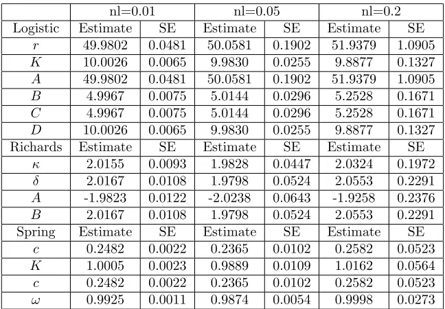
We compared the results for the asymptotic ellipsoids, exact ellipsoids, and DRAM Monte Carlo simulations side by side in Tables 5 - 11. This is done for each model (each parametrization of the logistic, Richards, and spring curves) and for each noise level (nl = 0.01,0.05,and 0.2). In order to better compare results, the plots for each model have the same axes across noise levels. Thus, for example, the logistic equation using the parameters (r, K) for noise level nl = 0.01 plots all have the same axes, but those axes will be different than those seen for the noise level nl= 0.05, or for the (A, B) parametrization. The axes used are always ˆθ±4·maxSE(ˆθk), where the standard errorsSE(ˆθk) can be found in Table 3.
nl=0.01 nl=0.05 nl=0.2 Logistic Estimate SE Estimate SE Estimate SE
r 49.9802 0.0481 50.0581 0.1902 51.9379 1.0905
K 10.0026 0.0065 9.9830 0.0255 9.8877 0.1327
A 49.9802 0.0481 50.0581 0.1902 51.9379 1.0905
B 4.9967 0.0075 5.0144 0.0296 5.2528 0.1671
C 4.9967 0.0075 5.0144 0.0296 5.2528 0.1671
D 10.0026 0.0065 9.9830 0.0255 9.8877 0.1327 Richards Estimate SE Estimate SE Estimate SE
κ 2.0155 0.0093 1.9828 0.0447 2.0324 0.1972
δ 2.0167 0.0108 1.9798 0.0524 2.0553 0.2291
A -1.9823 0.0122 -2.0238 0.0643 -1.9258 0.2376
B 2.0167 0.0108 1.9798 0.0524 2.0553 0.2291 Spring Estimate SE Estimate SE Estimate SE
c 0.2482 0.0022 0.2365 0.0102 0.2582 0.0523
K 1.0005 0.0023 0.9889 0.0109 1.0162 0.0564
c 0.2482 0.0022 0.2365 0.0102 0.2582 0.0523
ω 0.9925 0.0011 0.9874 0.0054 0.9998 0.0273
Table 3: Here we show the parameter estimates ˆθk and standard errors SE(ˆθk) for each parameterization for
each model at each noise level considered in this manuscript. Each row corresponds to a different parameter. For example, the second to last row corresponds to the parameter cin the (c, ω) parametrization for the spring equation, with the first two columns corresponding to the noise levelnl= 0.01, the next two columns corresponding to the noise levelnl= 0.05, and the last two columns corresponding to the noise levelnl= 0.2.
nl=0.01 nl=0.05 nl=0.2 Logistic (r, K) -0.7152 -0.7143 -0.6939 Logistic (A, B) 0.9529 0.9529 0.9527 Logistic (C, D) -0.8935 -0.8928 -0.8798 Richards (κ, δ) 0.9803 0.9798 0.9808 Richards (A, B) 0.9891 0.9899 0.9882 Spring (c, K) 0.3222 0.3222 0.3182 Spring (c, ω) 0.2131 0.2181 0.2047
Table 4: Here we show the correlation coefficientsρij for each parametrization of each model at each noise level
relationships. As expected from the definitions, the sign of the slope of the major axis in the asymptotic ellipsoids is given by the sign of the correlation coefficients in Table 4.
We compared results from the asymptotic ellipsoids to the correlation coefficient results. The asymptotic ellipsoids confirm what was seen with the correlation coefficients for the Richards curve and the spring equation. That is, the asymptotic ellipsoids for the Richards curve are diagonal, which suggests correlation in the estimators, while the asymptotic ellipsoids for the spring curve are not, which suggests no or little correlation in the estimators. For the logistic curve (r, K) parametrization, the asymptotic ellipsoid is vertical with an incredibly mild tilt, which would suggest little or no correlation in the estimators. When looking at the correlation coefficients we weren’t able to accurately determine whether there was strong correlation or not. For the logistic curve (C, D) parametrization, we see that the asymptotic ellipsoid has a pronounced diagonal tilt, which strongly suggests correlation in the estimators. The (A, B) parametrization of the logistic curve has a slightly sloped diagonal in the asymptotic ellipsoids, which suggests a slight correlation, while the correlation coefficients showed clear correlation. This confirms that the asymptotic ellipsoids provide a quick visualization of the information contained in the covariance matrices.
While the asymptotic ellipsoids and covariance matrices give information on the linear relationship of the estimators, the exact ellipsoids and DRAM Monte Carlo plots visually reveal any non-linear relationship of the estimators. In the results depicted here, a non-linear relationship only appears in the results for the (A, B) parametrization of the Richards curve, and it shows up very clearly in the exact ellipsoids and DRAM Monte Carlo plots as a banana shape (Table 9). It can be very difficult to determine a priori any non-linear relationship in the estimators, but the exact ellipsoids and DRAM methods are able to accurately reveal when there is.
nl Asymptotic Exact Dram
0.01
9.85 9.9 9.95 10 10.05 10.1 10.15
49.8 49.85 49.9 49.95 50 50.05 50.1 50.15
r
K
0.05
9.4 9.6 9.8 10 10.2 10.4 10.6
49.4 49.6 49.8 50 50.2 50.4 50.6 50.8
r
K
0.2 6 7 8 9 10 11 12 13 14
48 49 50 51 52 53 54 55 56
r
K
nl Asymptotic Exact Dram
0.01 49.8 49.85 49.9 49.95 50 50.05 50.1 50.15
4.85 4.9 4.95 5 5.05 5.1 5.15
B
A
0.05 49.4 49.6 49.8 50 50.2 50.4 50.6 50.8
4.4 4.6 4.8 5 5.2 5.4 5.6
B
A
0.2
48 49 50 51 52 53 54 55 56
1 2 3 4 5 6 7 8 9
B
A
nl Asymptotic Exact Dram
0.01
4.97 4.98 4.99 5 5.01 5.02
9.98 9.99 10 10.01 10.02 10.03
D
C
0.05 4.9 4.95 5 5.05 5.1
9.9 9.95 10 10.05 10.1
D
C
0.2
4.6 4.8 5 5.2 5.4 5.6 5.8
9.4 9.6 9.8 10 10.2 10.4
D
C
nl Asymptotic Exact Dram
0.01 1.98 1.99 2 2.01 2.02 2.03 2.04 2.05
1.98 1.99 2 2.01 2.02 2.03 2.04 2.05
κ
δ
0.05 1.8 1.85 1.9 1.95 2 2.05 2.1 2.15
1.8 1.85 1.9 1.95 2 2.05 2.1 2.15
κ
δ
0.2 1.2 1.4 1.6 1.8 2 2.2 2.4 2.6 2.8
1.2 1.4 1.6 1.8 2 2.2 2.4 2.6 2.8
κ
δ
nl Asymptotic Exact Dram
0.01 −2.02 −2 −1.98 −1.96 −1.94
1.97 1.98 1.99 2 2.01 2.02 2.03 2.04 2.05 2.06
B
A
0.05 −2.2 −2.1 −2 −1.9 −1.8
1.75 1.8 1.85 1.9 1.95 2 2.05 2.1 2.15 2.2
B
A
0.2 −2.5 −2 −1.5 −1
1.2 1.4 1.6 1.8 2 2.2 2.4 2.6 2.8 3
B
A
nl Asymptotic Exact Dram
0.01 0.240.242 0.244 0.246 0.248 0.25 0.252 0.254 0.256
0.992 0.994 0.996 0.998 1 1.002 1.004 1.006 1.008
K
C
0.05 0.2 0.21 0.22 0.23 0.24 0.25 0.26 0.27 0.28
0.95 0.96 0.97 0.98 0.99 1 1.01 1.02 1.03
K
C
0.2
0.05 0.1 0.15 0.2 0.25 0.3 0.35 0.4 0.45
0.8 0.85 0.9 0.95 1 1.05 1.1 1.15 1.2
K
C
nl Asymptotic Exact Dram
0.01
0.24 0.242 0.244 0.246 0.248 0.25 0.252 0.254 0.256
0.984 0.986 0.988 0.99 0.992 0.994 0.996 0.998 1
ω
C
0.05
0.2 0.21 0.22 0.23 0.24 0.25 0.26 0.27
0.95 0.96 0.97 0.98 0.99 1 1.01 1.02
ω
C
0.2
0.05 0.1 0.15 0.2 0.25 0.3 0.35 0.4 0.45
0.8 0.85 0.9 0.95 1 1.05 1.1 1.15 1.2
ω
C
Table 11: We plot the results for the spring equation with the (C, ω) parametrization. The left column of plots are the asymptotic ellipsoids, the middle column of plots are the exact ellipsoids, and the right column of plots are the DRAM Monte Carlo plots. The top row of plots correspond to noise levelnl = 0.01, the middle row to noise levelnl= 0.05, and the bottom row to noise levelnl= 0.2.
5
Discussion and Concluding Remarks
The considerations presented here arose from the simple question of what, if anything, we can say about de-pendence/independence of parameter estimators arising in inverse problems using simple computational methods related to estimator covariances. Initial findings with several simple one dimensional systems help to clarify the issues involved.
From the asymptotic theory-based covariances alone (see Table 2) which employ the linearized sensitivities in their construction, little definitive information can be obtained. If one computes the corresponding correlation coefficients, then in the extreme cases of ρnear zero (suggesting independence) or near ±1 (dependence) some useful information can be obtained about linear dependence. If one uses this along with the asymptotic based ellipsoids, information content can be enhanced in the non-extreme cases. If one turns to the exact ellipsoids (which are not computed using the linearized sensitivities), one can see not only linear dependence but a nonlinear dependence can be detected if present.
downside is this takes by far the longest to compute (at least for the examples considered here). Therefore, if all one needs is information about the correlation (or lack thereof) in parameter estimators (with an eye toward reparametrization), then we would not recommend using the DRAM algorithm in a first effort.
One should recognize that effort required in obtaining correlation information can be important factors in larger problems and that run times, and more meaningful measures such as function evaluations, ease in imple-mentation, etc., might be of interest. In that regard, it is important to note that there is a parallel implementation of DRAM [25], and also that the computation of the exact ellipsoids can be easily made parallel (in this note we only used serial implementations). If one considers more elaborate and computationally challenging mathematical models (e.g., such as the nonlinear models for HIV progression [4, 10], models for cell proliferation [7], climate models [23], nonlinear viscoelasticity [17], immune response in transplant patients [6]), then computational costs for the Bayesian approach [17, 23] could be an important consideration.
There are many limitations in our preliminary investigations: while the present study concerns itself ex-clusively with longitudal/repeated measurements [12] data, these preliminary insights are not limited to that situation; one only needs a system in which the assumptions of the asymptotic theory and Bayesian based DRAM apply. Moreover, we have not tried to apply optimal design techniques [1, 7, 8, 9] to obtain really efficient compu-tational schemes for the associated inverse problems in our comparisons. Finally we have not addressed at all the motivating issues [22, Chapter 3] of identifiability, ill-conditioning, and reparameterization for systems in which the parametertric estimators are found to exhibit dependence.
Acknowledgements
This research was supported in part by the Air Force Office of Scientific Research under grant number AFOSR FA9550-12-1-0188, in part by the National Science Foundation under Research Training Grant (RTG) DMS-1246991, NSF Undergraduate Biomathematics grant number DBI-1129214, and NSF grant number DMS-0946431.
References
[1] Kaska Adoteye, H.T. Banks and Kevin B. Flores, Optimal design of non-equilibrium experiments for genetic network interrogation, CRSC-TR14-12, N. C. State University, Raleigh, NC, September, 2014;Applied Math Letters,40(2015), 84–89.
[2] C. Andrieu and J. Thomas, A tutorial on adaptive MCMC,Statistics and Computing,18 (2008), 343–373. [3] A. Cintron-Arias, H.T. Banks, A. Capaldi and A. Lloyd, A sensitivity matrix based methodology for inverse
problem formulation,J. Inverse Ill-Posed Problems,17(2009), 545–564.
[4] H.T. Banks, R. Baraldi, K. Cross, C. McChesney, L. Poag, E. Thorpe, and K.B. Flores, Uncertainty quan-tification in modeling HIV viral mechanics, CRSC-TR13-16, N. C. State University, Raleigh, NC, December, 2013;Mathematical Biosciences and Engineering, 12(2015), to appear.
[5] H.T. Banks and B.G. Fitzpatrick, Statistical methods for model comparison in parameter estimation problems for distributed systems,J. Math. Biol.,28(1990), 501–527.
[6] H.T. Banks, S. Hu, K. Link, E.S. Rosenberg, S. Mitsuma and L. Rosario, Modeling immune response to BK virus infection and donor kidney in renal transplant recipients, CRSC-TR14-09, N. C. State University, Raleigh, NC, June, 2014;J. Inverse Problems in Science and Engineering, to appear.
[7] H.T. Banks, Shuhua Hu, and W. Clayton Thompson, Modeling and Inverse Problems in the Presence of Uncertainty,CRC Press, Boca Raton, FL, 2014.
[9] H.T. Banks and K.L. Rehm, Parameter estimation in distributed systems: Optimal design, CRSC TR14-06, N. C. State University, Raleigh, NC, May, 2014;Eurasian Journal of Mathematical and Computer Applica-tions,2(2014), 70-79.
[10] H.T. Banks and H.T. Tran, Mathematical and Experimental Modeling of Physical and Biological Processes, CRC Press, Boca Raton, FL, 2009.
[11] Y. Chu and J. Hahn, Parameter set selection for estimation of nonlinear dynamic systems,AIChE Journal, 53(2007), 2858–2870.
[12] M. Davidian and D.M. Giltinan, Nonlinear Models for Repeated Measurement Data, Chapman Hall/CRC Monographs on Statistics and Applied Probability, (1995).
[13] A.R. Gallant,Nonlinear Statistical Models, Wiley, New York, 1987.
[14] H. Haario, M. Laine, A. Mira, and E. Saksman, DRAM: Efficient adaptive MCMC,Statistics and Computing, 16.4(2006), 339–354.
[15] H. Haario, E. Saksman, and J. Tamminen, An adaptive Metropolis algorithm,Bernoulli,7.2(2001), 223–242. [16] J. Kaipio and E. Somersalo,Statistical and Computational Inverse Problems, Springer, New York, 2005.
[17] Zackary R. Kenz, H. T. Banks, and Ralph C. Smith. Comparison of frequentist and Bayesian confidence analysis methods on a viscoelastic stenosis model.SIAM/ASA Journal on Uncertainty Quantification, 1(1) (2013) 348–369.
[18] Joaquim R. R. A. Martins, Ilan M. Kroo, and Juan J. Alonso, An automated method for sensitivity anal-ysis using complex variables, Proc. 38th Aerospace Sciences Meeting, paper AIAA-2000-0689, Amer. Inst. Aeronautics and Astronautics (2000), pp. 1–12.
[19] R. Kent Nagle, Edward Saff, and Arthur Snider,Fundamentals of Differential Equations and Boundary Value Problems, Fourth edition, Pearson Education, Boston San Francisco New York, 2004.
[20] T.J. Rothenberg, Identification in parametric models, Econometrica,39(1971), 577-591. [21] G.A.F. Seber and A.J. Lee,Linear Regression Analysis, Wiley, Hoboken, 2003.
[22] G.A. Seber and C.J. Wild,Nonlinear Regression, Wiley, Hoboken, 2003.
[23] R.C. Smith, Uncertainty Quantification: Theory, Implementation, and Applications, SIAM, Philadelphia, 2014.
[24] A. Solonen,Monte Carlo Methods in Parameter Estimation of Nonlinear Models, MS Thesis, Lappeenranta University of Technology, Lappeenranta, Finland, 2006.
[25] A. Solonen, P. Ollinaho, M. Laine, H. Haario, J. Tamminen and H. J¨arvinen, Efficient MCMC for climate model parameter estimation: parallel adaptive chains and early rejection,Bayesian Analysis,7(2012), 715– 736.