ABSTRACT
LI, YIFANG. Bayesian Nonparametric Methods for Testing Shape Constraints. (Under the direction of Sujit K. Ghosh.)
In many applications, the relation between the covariates and the response variable is as-sumed to satisfy various shape constraints, such as monotonicity, convexity or combinations of both. For instance, demand and supply curves, cost and profit functions in econometrics, dose response curves in clinical trials and growth curves in biology are assumed to satisfy monotonicity. In such studies, it is natural to assume that the unknown regression function has pre-specified restrictions. It is also well known that by incorporating such constraints with appropriate justification, the estimation efficiency and power to detect the association can be improved.
Much literature has focused on the estimation of shape constrained regression functions. Sampling from a truncated multivariate distribution subject to multiple linear inequality con-straints is usually encountered in such problems in Bayesian framework, and also in many other areas in statistics and econometrics, such as the order restricted regressions, and censored data models. However, the sampling problem remains non-trivial due to the analytically intractable normalizing constant of the truncated multivariate distribution. In Chapter 1, we first develop an efficient rejection sampling method for the truncated univariate normal distribution, and an-alytically establish its superiority in terms of acceptance rates compared to some of the popular existing methods. We then extend our methodology to obtain samples from a truncated multi-variate normal distribution subject to convex polytope restriction regions. Finally, we generalize the sampling method to truncated scale mixtures multivariate normal distributions. Empirical results are presented to illustrate the superior performance of our proposed Gibbs sampler in terms of various criteria (e.g., accuracy, computing time, mixing and convergence rate).
In various cases, although a certain shape of the response is expected, due to the variability of the measurements or lack of scientific evidence, it may not be obvious to detect a specific shape of the trend using a scatter plot. This necessitates a formal statistical test to distinguish between a given class of possible shapes of a regression function (e.g., concave increasing vs. convex increasing etc.). Various tests have been explored within frequentist framework, however, the testing procedures are not so easy to implement in practice. In Chapter 2, we develop a nonparametric Bayesian method based on a sequence of penalized splines to test a general class of shapes of regression functions. The posterior consistency of the test is established rigorously and empirical results are presented to illustrate the simplicity and efficiency of the proposed method using simulated and real data sets.
data, we often have subject matter knowledge about the population that may suggest a specific shape of the unknown mean curve over a given time period of interest. However, due to the variability across subjects or sites, or lack of experimental scientific evidence, it may not be obvious to detect a specific shape of the population level trend based on sparsely observed data. A test of hypothesis of on such unknown shape constraints is hence of interest. A natural way to expand the Bayesian nonparametric test for unknown regression function presented in Chapter 2 is to use the aggregated data. However, this data aggregating approach does not work if the response variables are not sampled at the same time points across all subjects, which is commonly the case for longitudinal data sets. Mixed-effect model is a commonly used tool to account for variations across different subjects or sites. In Chapter 3, we develop a nonparametric Bayesian method to test various shape constraint of the population level mean trend based on approximating a Gaussian process using a sequence of penalized splines whose coefficients are allowed to vary with subjects or sites. Posterior consistency of the test procedure is established under a set of regularity conditions and numerical illustrations are presented based on simulated and real data sets.
Bayesian Nonparametric Methods for Testing Shape Constraints
by Yifang Li
A dissertation submitted to the Graduate Faculty of North Carolina State University
in partial fulfillment of the requirements for the Degree of
Doctor of Philosophy
Statistics
Raleigh, North Carolina
2015
APPROVED BY:
Subhashis Ghoshal Brian Reich
Yichao Wu Elon Ison
Sujit K. Ghosh
DEDICATION
BIOGRAPHY
Yifang Li was born on November 10th, 1985 in Jinan, Shandong, China, as the only daughter to parents Yinju Li and Wenke Ma.
With a software engineering father and an accountant mother, she developed deep interest in mathematics in her early age. Following her dream to become a mathematician, she attended Shandong University in her hometown majoring in Mathematics, with concentration in Statis-tics. Upon graduating from college, she decided to pursue her dream further and to take a chance to see the world. She went to Clemson University in Clemson, SC in 2008, and received an MS in Applied Mathematics. During her graduate study at Clemson University, she took more advanced courses in statistics, and completed a thesis on shrinkage estimation in partially linear models with measurement error, under the supervision of Drs. KB Kulasekera and Colin Gallagher, and found her passion in statistics. In 2010, she joined the Department of Statistics at North Carolina State University to pursue a PhD in statistics. Under the direction of Dr. Sujit K. Ghosh, she will graduate in August, 2015.
ACKNOWLEDGEMENTS
I would like to first express my deepest gratitude to my advisor, Dr. Sujit K. Ghosh, for it would have been impossible for this dissertation to be completed without his persistent patience, encouragement, and excellent guidance. I am extremely thankful to him for always being generous with his time to provide me help and direction for my research work out of his constant busy schedule, and for being flexible with the meeting time to accommodate my schedule of working part time at Quintiles. His profound and broad knowledge in statistics, and enthusiasm about finding ideas and solutions have been great inspiration throughout my PhD study.
I would like to thank Drs. Subhashis Ghoshal, Brian Reich, Yichao Wu, and Elon Ison for serving on my committee. They have raised interesting problems and provided valuable and insightful comments to my dissertation work, which greatly encourage me to pursue more achievement.
I would like to thank my boss at Quintiles, Russell Reeve, for being always supportive with my dissertation work, and being flexible with my working hours to accommodate my research progress. I am also grateful for his generosity of sharing with me his knowledge and experience in the pharmaceutical industry. The research of Chapter 4 in this dissertation is inspired by one of his many research ideas.
I would like to thank various faculty and staff members in Department of Statistics. Many thanks go to previous and current DGPs of our department, Drs. Pam Arroway, Jacqueline Hughes-Oliver, Sujit K. Ghosh, John Monahan, Howard Bondell and Kim Weems for generously providing direction and help at every step of my PhD study. I would also like to thank Lanakila Alexander, Adrian Blue and Alison McCoy for helping with all the paperwork and making the department feel like family.
I would like to thank my co-advisors at Clemson University, Drs. KB Kulasekera and Colin Gallagher for providing guidance and encouragement during my graduate study at Clemson University, and helped me discover my deep interest in statistics, which lead me to pursue a PhD in statistics at NC State.
TABLE OF CONTENTS
LIST OF TABLES . . . vii
LIST OF FIGURES . . . ix
Chapter 1 Efficient Sampling Methods for Truncated Multivariate Normal and Student-t Distributions Subject to Linear Inequality Constraints 1 1.1 Introduction . . . 1
1.2 Efficient Truncated Normal Sampling Method . . . 2
1.2.1 Algorithms for Truncated Univariate Normal Distributions . . . 4
1.2.2 Algorithm for Truncated Multivariate Normal Distributions . . . 11
1.3 Efficient Truncated Student-T Sampling Method . . . 13
1.4 Empirical performnaces . . . 14
1.4.1 Sampling from TUVN . . . 15
1.4.2 Sampling from TMVN and TMVT . . . 16
1.5 Conclusions and Discussions . . . 20
Chapter 2 Bayesian Nonparametric Methods to Test Shapes of Regression Functions . . . 23
2.1 Introduction . . . 23
2.2 Shape Constraints in Regression using P-splines . . . 25
2.2.1 Modeling with Bayesian P-splines . . . 26
2.2.2 Shape Constraints . . . 28
2.3 Testing Procedure and Posterior Consistency . . . 31
2.4 Simulation Studies . . . 38
2.5 Real Data Applications . . . 41
2.5.1 Dugong Growth Curve . . . 43
2.5.2 Global Temperature Anomalies Data . . . 44
2.6 Disscussion and Future Directions . . . 45
Chapter 3 Bayesian Nonparametric Methods to Test Shapes of Mixed Effect Models for Longitudinal Data . . . 49
3.1 Introduction . . . 49
3.2 A Gaussian Process Based Model for Longitudinal Data . . . 51
3.3 Approximation of GP Using P-splines . . . 54
3.4 Estimation with Bayesian P-splines . . . 59
3.5 Testing for Shape Constraints . . . 61
3.6 Simulation Studies . . . 66
3.7 Data Application . . . 67
3.8 Discussion and Future Directions . . . 70
Chapter 4 Model Based Approach to Test Biosimilars . . . 72
4.1 Introduction . . . 72
4.3 Test of Biosimilars . . . 85
4.4 Discussion and Future Directions . . . 88
References. . . 90
Appendices . . . 97
Appendix A Proofs of Lemmas in Chapter 1 . . . 98
A.1 Proof of Lemma 2 . . . 98
A.2 Proof of Lemma 3 . . . 99
A.3 Proof of Lemma 4 . . . 99
A.4 Proof of Lemma 5 . . . 100
A.5 Proof of Lemma 6 . . . 100
Appendix B Lemmas and Proofs in Chapter 2 . . . 101
B.1 Proof of Lemma 7 . . . 101
B.2 Lemmas Needed for Proof of Theorem 1 . . . 103
B.3 Proof of Lemma 9: . . . 105
B.4 Proof of Lemma 10: . . . 106
LIST OF TABLES
Table 1.1 Comparing empirical acceptance rates for Case 1 . . . 15 Table 1.2 Comparing empirical acceptance rates for Case 2 . . . 15 Table 1.3 Comparing empirical acceptance rates for Case 3 . . . 15
Table 2.1 Simulation results for σ2 = 0.01 based on 1000 Monte Carlo replications. BIC Freq. reports the frequency of eachk being selected in 1000 replications. Average posterior probability (Avg. Post. Prob.) is computed as the average of 1000 posterior probabilities defined in (2.33), with n = Mkn−2/7, where
Mnis calculated as in (2.32). Power is computed as the average of 1000 values
of δ defined in (2.34). . . 42 Table 2.2 Dugong growth curve data application. Post. Prob. of rejection reports the
posterior probability of rejectingH0with the proposed testing procedure given
in Theorem 1 computed as (2.33). The constant Mnfor testing for increasing
function is computed by (2.32).The constant for testing for concave increasing function is computed by (2.36). For comparison, posterior probabilities defined in (2.37) are also reported. Results are based on 10000 posterior draws with 1000 burn-in. BIC is computed using (2.35). . . 44 Table 2.3 Global temperature anomalies (1850-2012) data application. Post. Prob. of
rejection reports the posterior probability of rejecting H0 with the proposed
testing procedure given in Theorem 1 computed as (2.33). The constant Mn
for testing for increasing function is computed by (2.32).The constant for testing for concave increasing function is computed by (2.38). For comparison, posterior probabilities defined in (2.37) are also reported. Results are based on 10000 posterior draws with 1000 burn-in. BIC is computed using (2.35). . . 45 Table 2.4 Simulation results for σ2 = 0.01 based on 1000 Monte Carlo replications.
BIC Freq. reports the frequency of eachk being selected in 1000 replications. Average posterior probability (Avg. Post. Prob.) is computed as the average of 1000 posterior probabilities defined in (2.33), with n = Mnn−2/7, with
Mn is calculated as in (2.32), and n = Mn∗n−2/7, with Mn∗ is calculated as
in (2.39), respectively. Power is computed as the average of 1000 values of δ defined in (2.34) for two calibration methods. . . 48
Table 3.1 Simulation results based on 100 Monte Carlo replications. AIC and BIC Freq. reports the frequency of each k being selected in 100 replications. Average posterior probability of non-creasing (Avg. Post. Prob. of Non-increasing) computed as the average of 100 posterior probabilities defined in (2.33), with the cut-off value N defined in (3.29). . . 68
Table 3.2 Hearing loss data application. Post. Prob. of Non-increasing reports the pos-terior probability of rejecting H0 with the proposed testing procedure given
in Theorem 1 computed as (2.33). The cut-off value N for testing for
Table 4.1 Estimated asymptotes of each treatment, compared to Reeve et al. (2013). . . 80 Table 4.2 Time at which 50% of the largest asymptote (Etanercept high dose) is achieved
for a certain treatment, compared to Reeve et al. (2013). . . 80 Table 4.3 Margins for different time intervals based on the disease-progression models
of tocilizumab and MTX fitted in Section 4.2. . . 86 Table 4.4 Combinations of the asymptote ηb and the slope parameter γb of the test
biosimilar drug considered in the simulation study. . . 87 Table 4.5 Power the model-based approach on different time intervals compared to the
classic FDA approach, with sample size n0 =n1 = 100, based on 1000
simu-lated trials. . . 89 Table 4.6 Power the model-based approach on different time intervals compared to the
classic FDA approach, with sample size n0 =n1 = 280, based on 1000
LIST OF FIGURES
Figure 1.1 Comparing analytical acceptance rates for Case 1 . . . 9
Figure 1.2 Comparing analytical acceptance rates for Case 2 . . . 10
Figure 1.3 Comparing analytical acceptance rates for Case 3 . . . 11
Figure 1.4 Histograms of samples obtained for Case 1, 2 and 3 (µ= 2, σ= 1) in Section 1.4.1 . . . 16
Figure 1.5 Selected Contour plots when ρ= 0.5 in Example 1 . . . 18
Figure 1.6 Selected Contour plots when ρ= 0.98 in Example 1 . . . 18
Figure 1.7 Trace and ACF plots whenρ= 0.98 in Example 1 . . . 19
Figure 1.8 Trace and ACF plots whenρ= 0.98 by Geweke (1991)’s in Example 1 . . . . 20
Figure 1.9 Selected Trace and ACF plots whenρ= 0.5 by Geweke (1991)’s in Example 1 20 Figure 1.10 Histograms of generated samples with analytical marginal densities for the bounded region in Example 2 . . . 21
Figure 1.11 Histograms of generated samples with analytical marginal densities for the unbounded region in Example 2 . . . 21
Figure 1.12 Selected Trace and ACF plots for TMVT whenρ= 0.5, ν= 5 in Example 3 . 21 Figure 1.13 Selected Contour plots for TMVT when ρ= 0.5,ν = 5 in Example 3 . . . 22
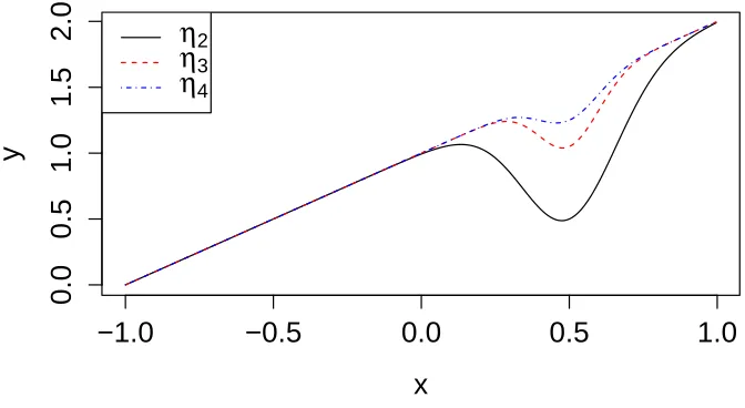
Figure 2.1 Shape comparisons of functions η2,η3 andη4 (see Equation (2.31)). . . 40
Figure 2.2 Dugong growth curve data and fitted curve, with 95% credible bands, based on 10000 posterior draws with 1000 burn-in. . . 44
Figure 2.3 Global temperature anomalies (1850-2012) data and fitted curve, with 95% credible bands, based on 10000 posterior draws with 1000 burn-in. . . 46
Figure 3.1 Berkeley growth data (Ramsay et al. (2014)). . . 50
Figure 3.2 Hearing thresholds for the right ear at 1 kHz (Davidov and Rosen (2011)). . 51
Figure 3.3 Verification of Assumption (A3.2) for the squared exponential kernel defined in (3.18). . . 59
Figure 3.4 Log-transformed hearing thresholds for the right ear at 1 kHz and the fitted mean function, with 95% credible bands, based on 10000 posterior draws with 1000 burn-in. . . 70
Figure 4.1 Examples of the innovator drug and test drugs using exponential models developed in Reeve et al. (2013). . . 74
Figure 4.2 ACR20 dose-response curves with model (4.7), with the data collected by Reeve et al. (2013). . . 79
Figure 4.3 ACR20 dose-response curves: Tocilizumab vs MTX . . . 81
Figure 4.4 ACR20 dose-response curves: Etanercept vs MTX . . . 81
Figure 4.5 ACR20 dose-response curves: Adalimumab vs MTX . . . 82
Figure 4.6 ACR20 dose-response curves: Golimumab vs MTX . . . 82
Figure 4.7 ACR20 dose-response curves: Infliximab vs MTX . . . 83
Figure 4.8 ACR20 dose-response curves: Certolizumab vs MTX . . . 83
Chapter 1
Efficient Sampling Methods for
Truncated Multivariate Normal and
Student-t Distributions Subject to
Linear Inequality Constraints
1.1
Introduction
The necessity of sampling from a truncated multivariate normal (TMVN) distribution subject to multiple linear inequality constraints arises in many research areas in statistics and econo-metrics. Robert (1995) gives several examples in the context of order restricted (or isotonic) regressions and censored data models. Several other applications are discussed by Gelfand et al. (1992), Liechty and Lu (2010) and Yu and Tian (2011), including the truncated multivariate probit models in market research, and modeling co-skewness of the skew-normal distributions, shape-restricted nonparametric regressions, and so on. The Bayesian normal linear regression model subject to linear inequality restrictions is also a common application of the TMVN dis-tributions, which is investigated in great details by Geweke (1996) and Rodrigues-Yam et al. (2004).
the fact that its marginal distributions are not TMVN and have very complicated pdf’s. Much research is done in seeking efficient sampling methods avoiding the evaluation of the normalizing constant.
The Gibbs sampler (Geman and Geman (1984) and Gelfand and Smith (1990)) has been a popular technique for sampling from TMVN distributions as all full conditional distributions of a TMVN are truncated univariate normal (TUVN) distributions. An early survey is provided by Hajivassiliou and Mcfadden (1990). Thus an efficient sampling method for TUVN is key in developing a sampling method for TMVN. Methods such as the classical inversion technique (Gelfand et al. (1992)) and naive rejection sampling using normal or uniform envelope functions (Breslaw (1994)) are recognized as not accurate or efficient in many cases. Geweke (1991) and Robert (1995) develop methods based on various combinations of standard rejection sampling methods for TUVN within the Gibbs sampler for TMVN. Both of these methods have low acceptance rates for certain types of restrictions. Geweke (1991)’s Gibbs sampler for TMVN suffers from slow convergence, and our empirical studies illustrate that this is especially the case for unbounded regions. Rodrigues-Yam et al. (2004) propose a type of transformation focusing on simplifying the covariance by uncorrelating the random vectors, which somewhat fix the poor mixing property of Geweke (1991)’s method. However, most of these previous work does not provide theoretical properties (e.g., acceptance rates of rejection sampling etc.).
In this chapter, we develop an efficient mixed rejection sampling method for TUVN distri-butions and a Gibbs sampler for TMVN distridistri-butions. The layout of the chapter is as follows. In Section 1.2, we describe our sampling methods for both of the TUVN and TMVN distributions. The analytical acceptance rates of the proposed mixed rejection sampling method for TUVN distributions are derived analytically and compared to Geweke (1991)’s and Robert (1995)’s methods. The results demonstrate that our method has uniformly larger analytical acceptance rates than both of the existing methods. This sampling method is generalized to truncated multivariate Student-t distribution (TMVT) in Section 1.3. In Section 1.4, we present the em-pirical acceptance rates for TUVN distributions. Further numerical examples with our Gibbs sampler for TMVN and TMVT distributions with various restriction regions are presented, to demonstrate the accuracy and the fast convergence of the proposed method. In Section 1.5, we provide conclusions and further discussions in this area. Proofs of the lemmas and additional tables and figures are provided in Appendix A.
1.2
Efficient Truncated Normal Sampling Method
normal distribution subject to linear inequality constraints, if its pdf is
fW(w) =
exp−1
2(w−µ)
TΣ−1(w−µ)
R
c≤Rw≤de exp
−1
2(w−µ)TΣ
−1(w−µ) dw I(c≤Rwe ≤d), (1.1)
whereΣis a non-negative definite matrix,I is the indicator function, andRe is am×pmatrix
with rank m ≤ p. The inequality notation of c ≤ Rwe ≤ d means that the inequality holds
element-wisely, i.e., ci ≤ [Rwe ]i ≤ di for each i = 1,2, . . . , m, withci’s and di’s allowed to be
−∞ and +∞, respectively. We denote this TMVN distribution asW ∼T Np(µ,Σ;Re,c,d).A
good collection of statistical properties of TMVN distributions can be found in Horrace (2005). We state two key properties of TMVN distributions, which enable the development of the proposed sampling methods.
Proposition 1. Let Y =AW, where A is a q×p matrix with rank q≤p. Then,
Y ∼T Nq(Aµ,AΣAT;T), (1.2)
where T ={Aw:c≤Rwe ≤d}.
Proposition 2. Partition X, µ andΣ as
X = X1
X2
!
, µ= µ1
µ2
!
, andΣ= Σ11 Σ12
Σ21 Σ22 !
.,
where X1 is a p1-dimensional random vector andX2 is a p2-dimensional random vector, and
p1+p2=p. Then the conditional distribution ofX1 given X2 =x2 is
X1|X2 =x2 ∼T Np1(µ1+Σ12Σ−122(x2−µ2),Σ11−Σ12Σ22−1Σ21;R1(x2)), (1.3)
where
R1(x2) =
(
x1∈Rp1 :a≤R x1
x2
!
≤b
)
.
A similar result holds for the conditional distribution of X2 given X1=x1.
It is worth mentioning that in both (1.2) and (1.3), the restriction regions may not be explicitly written in the form of c∗ ≤ Re
∗
x∗ ≤ d∗ for some Re ∗
, c∗ and d∗, however, the constraints are still linear inequalities.
1.2.1 Algorithms for Truncated Univariate Normal Distributions
In this section, we introduce our method for generating samples from a TUVN distribution. A random variableW is said to follow a TUVN distribution, if its pdf is
fW(w) =
1 σ φ
w−µ σ
Φ
d−µ σ
−Φ
c−µ σ
I(c≤w≤d) ∝ φ
w−µ σ
I(c≤w≤d), (1.4)
where φ denotes the pdf of N(0,1), and Φ denotes its cumulative distribution function (cdf). In the restriction, the boundsc and dare allowed to be −∞and +∞, respectively. We denote the distribution as W ∼T N(µ, σ2;c, d). It easily follows that
X= W −µ
σ ∼T N(0,1;a, b), (1.5)
wherea= (c−µ)/σ, andb= (d−µ)/σ, and the transformed random variableXhas the pdf given byfX(x) = Φ(bφ)−Φ((x) a)I(a≤x≤b).Notice that a sampled valuexgenerated from T N(0,1;a, b)
can be used to obtain a sample fromT N(µ, σ2;c, d) by the transformationw=σx+µ. Therefore,
without loss of generality, we establish an efficient sampling method for the standard TUVN random variableX.
Mixed Rejection Algorithm
In this section, we develop a new mixed accept-reject algorithm, by combining four standard rejection sampling methods with the goal of optimizing the acceptance rate uniformly.
Following the work of Geweke (1991) and Robert (1995), the proposed sampling algorithm is based on basic accept-reject algorithm, which is a common method for generating samples from a distribution. More details can be seen in Chapter 2 of Robert and Casella (2004). This algorithm is stated as a lemma below.
Lemma 1. To draw a sample fromX∼f(x), if for allx, there exists a constantM ≥1, and a known density functiong(x)defined on a common support with f(x), such thatf(x)≤M g(x), then it is sufficient to generate x∼g and u∼U nif[0,1], and until u ≤f(x)/(M g(x)), take x
as a sample fromf(x), . The resulting acceptance rate is then1/M, and this acceptance rate is maximized at Mopt= sup. x:g(x)>0
f(x)
g(x).
rejection sampling (ER). With the goal of maximizing the acceptance rate globally, we propose the following algorithm:
Proposed Algorithm for TUVN:
Case 1 For the truncated interval[a,∞); if
(i) a≤0: use the normal rejection sampling,
(ii) 0< a < a0: use the half-normal rejection sampling,
(iii) a≥a0: use the one-sided translated-exponential.
Case 2 For the truncated interval0∈[a, b]; if
(i) b≤a+√2π: use the uniform rejection sampling,
(ii) b > a+√2π: use the normal rejection sampling.
Case 3 For the truncated interval[a, b], a≥0; if
(i) 0≤a < a0, and if
(a) b≤b1(a): use the uniform rejection sampling,
(b) b > b1(a): use the half-normal rejection sampling;
(ii) a≥a0, and if
(a) b≤b2(a): use the uniform rejection sampling,
(b) b > b2(a): use the two-sided translated-exponential rejection sampling.
Case 4 For the truncated interval (−∞, b]: use the symmetric algorithm to Case 1.
Case 5 For the truncated interval[a, b], b≤0: use the symmetric algorithm to Case 3.
In the above algorithm, the constants are given bya0 = 0.2570,b1(a) =a+ pπ
2 exp n
a2
2 o
, and b2(a) = a+ a+√2a2+4exp
n
a2−a√a2+4
4 +
1 2
o
. We then show that this mixed accept-reject algorithm has globally optimal acceptance rates and is thus more efficient than those proposed by Geweke (1991) and Robert (1995).
Normal rejection sampling. Normal rejection sampling is a natural yet naive sampling method for TUVN, in which we set the envelope function g(x) = φ(x). Hence we draw a candidate x fromN(0,1), accept x as a sample of the TUVN if it is in the range of [a, b]. The resulting acceptance rate is
pN =. pN(a, b) = Φ(b)−Φ(a).
Here aand bare allowed to take the values as ±∞ respectively.
Half-normal rejection sampling. When a≥0, we can consider the half-normal rejection sampling. In this method, a candidatexis drawn fromN(0,1), retainxif|x| ∈[a, b]. It is easy to show that the acceptance rate is
pH =. pH(a, b) = 2(Φ(b)−Φ(a)).
Here b is allowed to be +∞. Notice that this is more efficient than normal rejection sampling when a≥0.
Uniform rejection sampling. When the interval is bounded, uniform distribution can be considered as the envelope distribution for sampling from TUVN distribution. We set g(x) = 1/(b−a) as the pdf of U nif[a, b]. Since φ(x) is maximized at x = 0 if x is unrestricted, the constant that maximizes the acceptance rate is given by Mopt= (b−a)φ{bIΦ((bb)−Φ(≤0)+aaI) (a≥0)}. Hence,
the corresponding acceptance rate is
pU,1 =. pU,1(a, b) =
√
2π
b−a(Φ(b)−Φ(a)), ifa≤0≤b;
pU,2 =. pU,2(a, b) =
√
2π b−ae
a2
2 (Φ(b)−Φ(a)), ifa≥0;
pU,3 =. pU,3(a, b) =
√
2π b−ae
b2
2 (Φ(b)−Φ(a)), ifb≤0.
Translated-exponential rejection sampling. The translated-exponential rejection sam-pling method is initially considered for the type of the one-side restriction intervals with the form of [a,∞] for a ≥ 0. The envelope density of this method is a a translated-exponential distribution with pdf
g(x) =λexp{−λ(x−a)}I(x≥a), (1.6)
Lemma 2. The maximized acceptance rate of the one-sided translated-exponential rejection sampling is
pE,1 =. pE,1(a, b) =
√
2πλ∗exp
−λ
∗2
2 +λ
∗a
Φ(−a),
where
λ∗=. λ∗(a) = a+
√
a2+ 4
2 . (1.7)
It is worth pointing out that, asaapproaches∞, the acceptance ratepE,1 goes to 1, which
illustrates that asa→ ∞, the translated-exponential distribution starts to resemble the TUVN distribution. Using λ∗ does not increase the computation time as for any given value of a, if the translated-exponential rejection sampling is chosen for that region, λ∗ only needs to be evaluated once.
The translated-exponential rejection sampling method can also be used for two-sided re-striction intervals as [a, b], provided that the upper boundbis relatively large. In the two-sided translated-exponential rejection sampling, the candidate x is generated from the translated-exponential distribution with pdf defined in (1.6), until x ≤ b. Following a similar procedure of maximizing the acceptance rate of the one-sided translated-exponential distribution (as in Lemma 2), we get the maximized acceptance rate for the two-sided case as
pE,2 =. pE,2(a, b) =
√
2π λ∗exp
λ∗a−1
2λ
∗2
(Φ(b)−Φ(a)).
Now we compare the four basic rejection sampling methods using a case-by-case approach by maximizing the acceptance probability for all restriction intervals. Based on the different natures and suitabilities of the basic rejection sampling methods, the restriction intervals are divided into five categories as listed in the algorithm. Note that the sampling method of TUVN with restriction region [−b,−a] can be directly derived from the method for the restriction region [a, b]. To sample x ∼ T N(0,1;−b,−a), one can generate y ∼ T N(0,1;a, b), and take x = −y. In this sense, we call the regions [a, b] and [−b,−a] symmetric to each other. The above argument also holds whena=−∞, orb=∞. Hence, Case 4 is symmetric to Case 1, and Case 5 to Case 3. Therefore, we focus on optimizing the sampling methods for the first three cases.
It is well known that naively using only NR is impractical for TUVN sampling method. NR may work well when the mean 0 is contained in the region [a, b]. When a is several standard deviations away to the right of 0, NR is very inefficient. For the one-sided region, NR is only valid when a ≤ 0. Note that pH is uniformly larger than pN, hence HR is favored over NR
preferred, as the shape mimics the TUVN distribution better. We now explore the four basic rejection sampling methods and obtain the best acceptance rates.
Case 1. When a≤ 0, NR is the only available method for the one-sided restriction regions. Whena >0, both HR and ER are also candidates, but with higher acceptance rates than NR. Therefore, we only consider these two methods whena >0. The comparison between them is stated in the following lemma, and it results the choice of envelope functions stated in the algorithm.
Lemma 3 (HR vs. ER). For the one-sided region with the form [a,∞) with a≥0, there exists a0 >0, such that when 0< a < a0, pH > pE. When a≥a0, pE ≥pH. In above, a0 is the solution of the equation
λ∗eλ
∗2
2 −1 =
r
2 π,
which is approximately0.2570 (up to 4 decimal places), and λ∗ is given as in (1.7).
Case 2. For this type of two-sided finite restriction regions, only NR and UR are suitable. The results of comparing the acceptance rates of the two methods are given in the lemma below and the choice of envelope functions for this case follows.
Lemma 4 (NR vs. UR). For the two-sided region with the form [a, b], where a <0< b, when b−a≤√2π, pU,1 ≥pN; when b−a >
√
2π, pN > pU,1.
Case 3. This type of two-sided regions require the most detailed comparative analysis since all four rejection sampling methods are available. However, aspH is uniformly larger thanpN
for anya and b, we do not consider NR for this case. We then focus on the comparisons among the other three methods and the results are stated as follows.
Lemma 5(HR vs. UR). For the two-sided regions with the form[a, b], wherea≥0, when
b < a+
r
π 2 exp
a2 2
. =b1(a),
pU,2 > pH. Otherwise, pH ≥pU,2.
Lemma 6 (UR vs. ER). For the two-sided regions with the form [a, b], where a≥0, if
b≤a+ 2
a+√a2+ 4exp (
a2−a√a2+ 4
4 +
1 2
)
.
=b2(a), (1.8)
Combining Lemma 3, Lemma 5, and Lemma 6, for Case 3, we first discriminate the situations according to the comparison between HR and ER, as this comparison only involves the value of a, and then consider the comparison between UR and ER. As we always favor the method with larger acceptance rate, the choice stated in the algorithm results.
Comparisons of Analytical Acceptance Rates
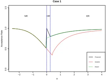
Our studies show that generally, Robert (1995)’s method outperforms Geweke (1991)’s for Case 1 and Case 3, while the dominance reverses for Case 2, in terms of acceptance rates. To compare the acceptance rates of the proposed method with the two existing ones, we plot them for Case 1 to 3, shown in Figures 1.1 to 1.3. As the switching criteria for Cases 2 and 3 involves both aand b, we present some representative values of a for illustration. These figures clearly show the sub-optimal performance in acceptance rates of the two widely used existing methods.
−2 −1 0 1 2 3 4
0.0
0.5
1.0
1.5
Case 1
a
Acceptance Rate
NR HR ER
Proposed Geweke Robert
Figure 1.1: Comparing analytical acceptance rates for Case 1
Generally speaking, in Geweke (1991)’s algorithm, there are four ad-hoc constants serving as critical values of deciding which of the four basic rejection sampling methods to be used. However, theoretical analysis shows that this ad-hoc choice may cause very low acceptance rates in some cases. Moreover, in Case 2 and 3, Geweke (1991)’s switching criteria involve evaluations of φ(a) and φ(b), which may also cause low efficiency when using in a Gibbs sampler. As for Robert (1995)’s method, HR is not considered, hence the algorithm does not take advantage of the similar nature of the half-normal distributions to the TUVN when the lower bound is close to 0 for one-sided regions, or for relatively wide bounded regions.
0 1 2 3 4 5
0.0
0.5
1.0
1.5
Case 2, a= −2
b
Acceptance Rate
UR NR
Proposed Geweke Robert
0 1 2 3 4 5
0.0
0.5
1.0
1.5
Case 2, a= −1
b
Acceptance Rate
UR NR
Proposed Geweke Robert
0 1 2 3 4 5
0.0
0.5
1.0
1.5
Case 2, a= −0.5
b
Acceptance Rate
UR NR
Proposed Geweke Robert
0 1 2 3 4 5
0.0
0.5
1.0
1.5
Case 2, a= −0.1
b
Acceptance Rate
UR NR
Proposed Geweke Robert
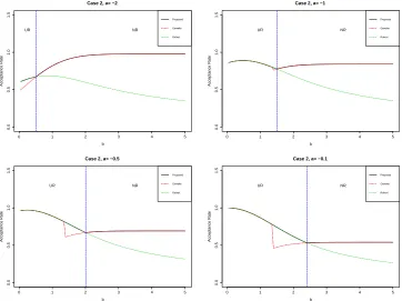
Figure 1.2: Comparing analytical acceptance rates for Case 2
of the other two methods. Note that when a = 0, our acceptance rate is exactly 1, because T N(0,1; 0,∞) is exactly the half-normal distribution. For this case, Robert (1995) uses ER with acceptance rate 0.760, and Geweke (1991) uses the naive NR with acceptance rate 0.500. In Geweke (1991)’s method, the value separating NR and ER (non-optimal) is 0.45, and the resulted acceptance rate is as low as 0.326, compared to ours at 0.822, which illustrates that Geweke (1991)’s choice of the four constants is not optimal.
In Figure 1.2 for Case 2, acceptance rates are plotted for four values of a. The blue lines indicate the switching valuea+√2π, depending ona. This figure gives a clear illustration that UR only performs well for narrow restriction intervals. However, it is the only sampling method used by Robert (1995) for this case. Although Geweke (1991) uses the similar idea as ours, since the switching criteria are not optimized, it has smaller acceptance rates for relatively narrow regions.
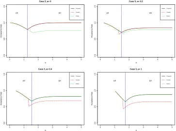
In Figure 1.3 for Case 3, acceptance rates of four values of aare plotted, two of which are less than a0 = 0.2570, two of which are larger. The switching value indicated by the blue line
is b1(a) fora less than a0, and b2(a) otherwise. When 0≤a < a0, Robert (1995)’s acceptance
0 1 2 3 4 5
0.0
0.5
1.0
1.5
Case 3, a= 0
b
Acceptance Rate
UR HR
Proposed Geweke Robert
0 1 2 3 4 5
0.0
0.5
1.0
1.5
Case 3, a= 0.2
b
Acceptance Rate
UR HR
Proposed Geweke Robert
0 1 2 3 4 5
0.0
0.5
1.0
1.5
Case 3, a= 0.4
b
Acceptance Rate
UR ER
Proposed Geweke Robert
0 1 2 3 4 5
0.0
0.5
1.0
1.5
Case 3, a= 1
b
Acceptance Rate
UR ER
Proposed Geweke Robert
Figure 1.3: Comparing analytical acceptance rates for Case 3
uses either HR or ER (non-optimal) for wide regions. Due to the choice of envelope functions, the acceptance rates are low for certain regions.
These comparisons demonstrate how the proposed method outperforms the two existing ones. Moreover, as the proposed method does not involve much complicated computations, the running time is similar to that of the other existing methods when sampling TUVN alone.
1.2.2 Algorithm for Truncated Multivariate Normal Distributions
Now that we have an efficient sampling method for TUVN distributions, we focus on the sampling method for the TMVN distribution, which is the central interest of this chapter.
To simplify the procedure of the Gibbs sampler, usually some transformations are done before the Gibbs sampler is implemented. For any general TMVN distributed random vector
W ∼T Np(µ,Σ;Re,c,d), Geweke (1991) proposes to use the transformation asZ=Re(W−µ).
The motivation behind this is that the resulting restrictions of the random vector Z becomes
α≤Z≤β, where α=a−Rµe and β=b−Rµe , hence the restrictions are explicitly defined
for every component without any linear summation involved. Although this transformation simplifies the restrictions, the distribution ofZisT Np(0,ReΣRe
T
matrix is complicated. The resulting full conditional distributions required within the Gibbs sampler are not truncated standard univariate normal. As the sampling method is defined for T N(0,1;a, b) only, in each of the Gibbs updating step, two transformations are required, one of which is to transform the nonstandard TUVN to the standard TUVN, and another one is to transform the generated sample back to the original full conditional distribution for later updating steps, and in each of the step, one matrix inversion is needed. This causes inefficiency in Geweke (1991)’s sampling method for TMVN especially when a large number of samples are of interest from a high dimensional TMVN distribution. The non-diagonal covariance matrix is also a source for the poor mixing in the Gibbs sampler. Moreover, since the backward transformation is needed, the matrix Re is required to be squared and invertible, which limits the application
of the method.
To improve the mixing, we introduce the transformation as
X =Σ−1/2(W −µ), (1.9)
whereΣ−1/2 denotes the inverse ofΣ1/2, which is the lower triangular Cholesky decomposition of the covariance matrix Σ. According to Proposition 1, X ∼ T Np(0,I;R,a,b), with R =
e
RΣ1/2,a=c−Rµe , andb=d−Reµ. This transformation greatly simplifies the pdf given in
(1.1), instead of only the constraints of the TMVN distribution. As a result, we do not require
e
R to be an invertible matrix, and hence allow that m≤p with linearly independent rows. By Proposition 2, the resulted full univariate conditional distribution is
xi|x−i ∼T N(0,1;a∗i(x−i), b∗i(x−i)), i= 1, . . . , p, (1.10)
wherex−i = (x1, . . . , xi−1, xi+1, . . . , xp), anda∗i(x−i) andb∗i(x−i) are determined suitably such
that a ≤ Rx ≤ b. The full conditional distribution described in (1.10) shows the advantage of making such a transformation, that in each updating step of the Gibbs sampler, we deal with a truncated standard univariate normal distribution. This procedure improves the poor mixing of the Gibbs sampler proposed by Geweke (1991), especially for wider restriction regions. Without loss of generality, we develop the sampling method for the random vectorX. To obtain the samples for the original TMVN vector W, we simply use the following transformation
w = Σ1/2x+µ, where x is obtained by the Gibbs sampling. Our method only requires two linear matrix transformations, and one matrix inversion in the Cholesky decomposition of the covariance matrix.
We next explain how to evaluate the lower and the upper boundsa∗i andb∗i in every updating step. LetRi denote the ith column of R,R−i denote the m×(p−1) matrix by removing the
b−R−ix−i, which is equivalent to the following coordinate-wise inequalities
aj−rj,−ix−i≤rjixi ≤bj −rj,−ix−i, j = 1, . . . , m, (1.11)
whererj,−i denotes thejth row of the matrix R−i, and rji denotes the jth entry of the vector Ri. Depending on the sign ofrji, we have three different scenarios:
When rji>0. For all j’s such that rji > 0, (1.11) is equivalent to
aj−rj,−ix−i
rji ≤ xi ≤
bj−rj,−ix−i
rji . Hence we definel
+
i = max{j:rji>0}
aj−rj,−ix−i
rji andu
+
i = min{j:rji>0}
bj−rj,−ix−i
rji .
When rji<0. For all j’s such that rji < 0, (1.11) is equivalent to bj−rj,rji−ix−i ≤ xi ≤
aj−rj,−ix−i
rji .Hence we definel
−
i = maxj:rji<0
bj−rj,−ix−i
rji and u
−
i = minj:rji<0
aj−rj,−ix−i
rji .
When rji= 0. There is no restriction on xi for this j.
Combining all three scenarios discussed above, we have
a∗i = max{l+i , l−i } and b∗i = max{u+i , u−i }.
Ifa∗i ≤b∗i, these bounds can be used for sampling from the full conditional distribution in each step of the Gibbs sampler. In fact, the region defined by{x:a≤Rx≤b}is a convex polytope. Hence as long as the starting value is within the region, our method remains feasible in every updating step. Therefore, in the ith step of the tth pass in the Gibbs sampler, we sample
xi(t)|x1(t), . . . , x(it−1) , xi(+1t−1), . . . , x(pt−1) ∼T N(0,1;a∗(i t), b∗(i t)), (1.12)
wherea∗(i t)=a∗i(x1(t), . . . , x(i−1t) , x(i+1t−1), . . . , x(pt−1)), andb∗(i t)=bi∗(x(1t), . . . , x(it−1) , x (t−1)
i+1 , . . . , x (t−1)
p ),
fori= 1, . . . , p.
Empirical results in Section 1.4 demonstrate that the proposed Gibbs sampler has very good mixing property and converges fast to the true truncated multivariate normal distribution.
1.3
Efficient Truncated Student-T Sampling Method
A random vector Y following a truncated multivariate (p-variate) Student-t distribution with degree of freedomν subject to linear inequality constraintsc≤Rye ≤d is denoted as
Y ∼T Tp(µ,Σ, ν;Re,c,d).
Following the property of a multivariate Student-t distribution, a similar transformation as in (1.9) can be done such thatT =Σ−1/2(Y −µ)∼T Tp(0,I, ν;R,a,b),whereΣ−1/2,R,a, and bare defined as before. Therefore, without loss of generality, we develop the sampling algorithm forT. To obtain a sample y of the distribution of Y from a sample t of T, we only require a simple transformation as y=Σ1/2t+µ.
Let T∗ ∼Tp(0,I, ν) denote an untrucated p-variate Student-t distributed random variable
with degree of freedomν, then by definition,T∗= √X∗
U/ν, whereX
∗∼N
p(0,I) is a standard
p-variate normal distributed random variable, andU ∼χ2(ν) is a chi-squared distributed random variable with degree of freedom ν, independent of X∗. Hence, for a given sample u from the distribution of U, the linear constraints of T can be expressed by a≤RT = √RX
u/ν ≤b, which
implies thatapu/ν ≤RX ≤bpu/ν. These facts indicate that a Gibbs sampler can be used to sample from TMVT distributions based on the existing TMVN sampling method.
The algorithm of the Gibbs sampler to obtain a sample t from T Tp(µ,Σ, ν;Re,c,d) is
de-scribed as follows:
1. Sample u∼χ2(ν).
2. Sample x∼T Np(0,I;R,a
p
u/ν,bpu/ν).
3. Set t= √x
u/ν.
In the second step, our proposed Gibbs sampler for TMVN sampling will be implemented. As the efficiency and accuracy of the TMVT distributions are highly influenced by that of the TMVN distributions, empirical studies given in Section 1.4 illustrate that this Gibbs sampler inherits the good mixing property and fast convergence from the sampling method for TMVN distributions.
1.4
Empirical performnaces
Table 1.1: Comparing empirical acceptance rates for Case 1
a New Geweke Robert a New Geweke Robert -2 0.977 0.977 0.977 0.2 0.840 0.421 0.790 -1 0.840 0.840 0.840 0.45 0.823 0.324 0.823 -0.5 0.695 0.695 0.695 1 0.880 0.656 0.880 0 1.000 0.495 0.763 5 0.984 0.969 0.984
Table 1.2: Comparing empirical acceptance rates for Case 2
New Geweke Robert New Geweke Robert
b a=−2 a=−1
.5 0.672 0.660 0.672 0.897 0.897 0.897 1 0.819 0.819 0.687 0.860 0.860 0.860 2 0.954 0.954 0.606 0.819 0.819 0.690
b a=−0.5 a=−0.1
2 0.680 0.673 0.680 0.624 0.515 0.624
1.4.1 Sampling from TUVN
We first present the empirical results for the proposed mixed rejection sampling algorithm for TUVN distributions.
As mentioned previously, in terms of acceptance rates, Robert (1995)’s algorithm outper-forms Geweke (1991)’s for Case 1 and Case 3, and vice versa for Case 2. As a result, it is of interest to compare our proposed algorithm with Robert (1995)’s for Cases 1 and 3, and with Geweke (1991)’s for Case 2. The empirical acceptance rates for some representative regions are listed in Tables 1.1 through 1.3. For each of the restriction intervals, 10,000 samples are gener-ated using three methods: the newly proposed method, Geweke (1991)’s, and Robert (1995)’s. For each method, the empirical acceptance rates are computed as 10,000/Ntry, where Ntry
denotes the total number of trials until 10,000 samples are accepted.
Figure 1.4 is the histograms of the samples obtained by the proposed algorithm with the exact density curves overlayed forT N(2,1;c, d). The bounds are provided in the captions of the figures. It clearly indicates that sampling distribution captures the true shape of the density of the TUVN. In addition to depicting histograms, we also carried out a few standard goodness of fit tests (Anderson-Darling, Kolmogorov-Smirnov, etc), all of which further confirms the correct generating mechanism of the proposed method.
Table 1.3: Comparing empirical acceptance rates for Case 3
New Geweke Robert New Geweke Robert New Geweke Robert
b a= 0 b a= 1 b a= 2
lower= 2 upper= Inf
x
Density
2 3 4 5 6
0.0
0.2
0.4
0.6
0.8
lower= 0 upper= Inf
x
Density
0 1 2 3 4 5 6
0.0
0.1
0.2
0.3
0.4
lower= 3 upper= Inf
x
Density
3.0 4.0 5.0 6.0
0.0
0.4
0.8
1.2
lower= 7 upper= Inf
x
Density
7.0 7.5 8.0 8.5
0
1
2
3
4
(a) Case 1
lower= 0 upper= 2.5
x
Density
0.0 0.5 1.0 1.5 2.0 2.5
0.0
0.2
0.4
0.6
lower= 1 upper= 3
x
Density
1.0 1.5 2.0 2.5 3.0
0.0
0.2
0.4
0.6
lower= 1 upper= 4
x
Density
1.0 1.5 2.0 2.5 3.0 3.5 4.0
0.0
0.2
0.4
lower= 1.5 upper= 4
x
Density
1.5 2.0 2.5 3.0 3.5 4.0
0.0
0.2
0.4
0.6
(b) Case 2
lower= 2 upper= 4
x
Density
2.0 2.5 3.0 3.5 4.0
0.0
0.2
0.4
0.6
0.8
lower= 2 upper= 2.5
x
Density
2.0 2.1 2.2 2.3 2.4 2.5
0.0
0.5
1.0
1.5
2.0
lower= 3 upper= 4
x
Density
3.0 3.2 3.4 3.6 3.8 4.0
0.0
0.5
1.0
1.5
lower= 2.5 upper= 6
x
Density
2.5 3.5 4.5 5.5
0.0
0.4
0.8
(c) Case 3
Figure 1.4: Histograms of samples obtained for Case 1, 2 and 3 (µ= 2, σ= 1) in Section 1.4.1
1.4.2 Sampling from TMVN and TMVT
We illustrate our sampling method for several examples to explore how well our method works for different types of TMVN and TMVT distributions.
Example 1. In this example, we apply our method to truncated bivariate normal (TBVN) distributions. For TBVN, we are able to display the accuracy of the sampling method on a contour plot of the distribution. This is difficult for higher dimensional TMVN distributions due to the property that the marginal distributions are not TMVN and have very complex pdf’s.
Consider a random vectorX = (X1, X2)T withµ= (0,0)T,V ar(X1) = 10,V ar(X2) = 0.1,
and correlationρbetween two components. We investigate 6 different restriction regions. Define σ1 =
p
V ar(X1+X2), σ2 = p
V ar(X1−X2), and sd = (σ1, σ2)T. In the first 3 cases, the
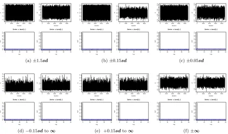
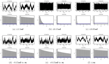
restriction regions are bounded in which X is truncated by ±1.5sd, ±0.15sd, and ±0.05sd, respectively. The fourth and the fifth restriction regions are one-sided open regions, with the lower bounds set to be−0.15sdand 0.15sd, respectively, and the upper bounds both set to be +∞. The sixth is an extreme case where the lower and the upper bounds are set to be ±∞, hence it is in fact an ordinary bivariate normal distribution. For each of the restriction regions, we test a moderate correlation ρ= 0.5, and a very high correlationρ= 0.98. The initial values for the fifth case is (1,0)T, while those of all the others are (0,0)T. Results are based on 10,000 generated samples and 1,000 burn-ins.
generated samples stay within the restricted regions, and sample points distribute according to the steps of the contour lines, which illustrates that the Gibbs sampler converges to target distribution.
Trace plots and auto-correlation function(ACF) plots are good visual indicators of the mix-ing property, which indicates how fast the MCMC chain converges to the stationary distribu-tion. High correlations between two components may cause poor mixing. Note that even when ρ= 0.98, Figure 1.7 illustrates that our Gibbs sampler has very good mixing property and the chains converge fast to the true densities. This is the case for all scenarios using the proposed Gibbs sampler. We also apply the Gibbs sampler proposed by Geweke (1991) using theR
func-tionrtmvnormin packagetmvtnorm. For most of the scenarios, especially unbounded restriction
regions and wider bounded restriction regions, even when the truncation is very moderate such as±1.5sd, this Gibbs sampler has poor mixing property and the chains converge very slowly, as seen in Figure 1.8. Changing to a lower correlation ρ = 0.5 improves the mixing property and accelerate the convergence for Geweke (1991)’s method. But the mixing is still not very satisfactory even for moderate truncated restriction regions as the trace plots are sticky and the ACF’s decay to 0 fairly slowly, as seen in Figure 1.9. These results strongly illustrate that our Gibbs sampler fixes the poor mixing property and slow convergence caused by Geweke (1991)’s method.
−4 −2 0 2 4
−1.0
−0.5
0.0
0.5
1.0
(a)±1.5sd
0 5 10
−1.0
−0.5
0.0
0.5
1.0
(b)−0.15sdto∞
Figure 1.5: Selected Contour plots whenρ= 0.5 in Example 1
−4 −2 0 2 4
−1.0
−0.5
0.0
0.5
1.0
(a)±1.5sd
0 5 10
0.0
0.5
1.0
1.5
(b)−0.15sdto∞
Figure 1.6: Selected Contour plots whenρ= 0.98 in Example 1
Example 2. In this example, we consider a 3-dimentional TMVN with the linear constraint matrixRe having smaller rank than the dimension, which is given as
µ=
0 0 0
, Σ=
1 0.5 0.25
0.5 1 0.5
0.25 0.5 1
, and ˜R=
1 −2 0
−1 0 0
!
.
0 2000 4000 6000 8000 −4 −2 0 2 4 Iteration x1
0 2000 4000 6000 8000
−0.6 −0.2 0.2 0.4 0.6 Iteration x2
0 10 20 30 40
0.0 0.2 0.4 0.6 0.8 1.0 Lag A CF
Series x_burn[1, ]
0 10 20 30 40
0.0 0.2 0.4 0.6 0.8 1.0 Lag A CF
Series x_burn[2, ]
(a)±1.5sd
0 2000 4000 6000 8000
−0.4 −0.2 0.0 0.2 0.4 Iteration x1
0 2000 4000 6000 8000
−0.2 −0.1 0.0 0.1 0.2 Iteration x2
0 10 20 30 40
0.0 0.2 0.4 0.6 0.8 1.0 Lag A CF
Series x_burn[1, ]
0 10 20 30 40
0.0 0.2 0.4 0.6 0.8 1.0 Lag A CF
Series x_burn[2, ]
(b)±0.15sd
0 2000 4000 6000 8000
−0.15 −0.05 0.05 0.15 Iteration x1
0 2000 4000 6000 8000
−0.15 −0.05 0.05 0.15 Iteration x2
0 10 20 30 40
0.0 0.2 0.4 0.6 0.8 1.0 Lag A CF
Series x_burn[1, ]
0 10 20 30 40
0.0 0.2 0.4 0.6 0.8 1.0 Lag A CF
Series x_burn[2, ]
(c)±0.05sd
0 2000 4000 6000 8000
0 2 4 6 8 10 12 14 Iteration x1
0 2000 4000 6000 8000
0.0
0.5
1.0
Iteration
x2
0 10 20 30 40
0.0 0.2 0.4 0.6 0.8 1.0 Lag A CF
Series x_burn[1, ]
0 10 20 30 40
0.0 0.2 0.4 0.6 0.8 1.0 Lag A CF
Series x_burn[2, ]
(d) −0.15sdto∞
0 2000 4000 6000 8000
2 4 6 8 10 12 Iteration x1
0 2000 4000 6000 8000
0.0 0.4 0.8 1.2 Iteration x2
0 10 20 30 40
0.0 0.2 0.4 0.6 0.8 1.0 Lag A CF
Series x_burn[1, ]
0 10 20 30 40
0.0 0.2 0.4 0.6 0.8 1.0 Lag A CF
Series x_burn[2, ]
(e) +0.15sdto∞
0 2000 4000 6000 8000
−10 −5 0 5 10 Iteration x1
0 2000 4000 6000 8000
−1.0 0.0 0.5 1.0 Iteration x2
0 10 20 30 40
0.0 0.2 0.4 0.6 0.8 1.0 Lag A CF
Series x_burn[1, ]
0 10 20 30 40
0.0 0.2 0.4 0.6 0.8 1.0 Lag A CF
Series x_burn[2, ]
(f)±∞
Figure 1.7: Trace and ACF plots whenρ= 0.98 in Example 1
histograms of the generated samples with the marginal densities are given by Figures 1.10 and 1.11. These figures not only show that our Gibbs sampler gives a correct and accurate sampling method, but also reveals the interesting effects resulted by truncation. In both of the cases, the marginal distributions of X1 and X2 are clearly skewed, while those ofX3 are symmetric and
appear to be normally distributed, which is expected because no constraints are imposed on X3.
0 2000 4000 6000 8000 −4 −2 0 2 4
X1 Trace Plot
Iteration
x1
0 2000 4000 6000 8000
−0.6
−0.2
0.2
0.4
X2 Trace Plot
Iteration
x2
0 10 20 30 40
0.0 0.2 0.4 0.6 0.8 1.0 Lag A CF
X1 ACF Plot
0 10 20 30 40
0.0 0.2 0.4 0.6 0.8 1.0 Lag A CF
X2 ACF Plot
(a)±1.5sd
0 2000 4000 6000 8000
−0.4
−0.2
0.0
0.2
0.4
X1 Trace Plot
Iteration
x1
0 2000 4000 6000 8000
−0.2
−0.1
0.0
0.1
0.2
X2 Trace Plot
Iteration
x2
0 10 20 30 40
0.0 0.2 0.4 0.6 0.8 1.0 Lag A CF
X1 ACF Plot
0 10 20 30 40
0.0 0.2 0.4 0.6 0.8 1.0 Lag A CF
X2 ACF Plot
(b)±0.15sd
0 2000 4000 6000 8000
−0.15
−0.05
0.05
0.15
X1 Trace Plot
Iteration
x1
0 2000 4000 6000 8000
−0.15
−0.05
0.05
0.15
X2 Trace Plot
Iteration
x2
0 10 20 30 40
0.0 0.2 0.4 0.6 0.8 1.0 Lag A CF
X1 ACF Plot
0 10 20 30 40
0.0 0.2 0.4 0.6 0.8 1.0 Lag A CF
X2 ACF Plot
(c)±0.05sd
0 2000 4000 6000 8000
0 1 2 3 4 5
X1 Trace Plot
Iteration
x1
0 2000 4000 6000 8000
−0.2
0.0
0.2
0.4
0.6
X2 Trace Plot
Iteration
x2
0 10 20 30 40
0.0 0.2 0.4 0.6 0.8 1.0 Lag A CF
X1 ACF Plot
0 10 20 30 40
0.0 0.2 0.4 0.6 0.8 1.0 Lag A CF
X2 ACF Plot
(d) −0.15sdto∞
0 2000 4000 6000 8000
1 2 3 4 5 6
X1 Trace Plot
Iteration
x1
0 2000 4000 6000 8000
0.0
0.2
0.4
0.6
X2 Trace Plot
Iteration
x2
0 10 20 30 40
0.0 0.2 0.4 0.6 0.8 1.0 Lag A CF
X1 ACF Plot
0 10 20 30 40
0.0 0.2 0.4 0.6 0.8 1.0 Lag A CF
X2 ACF Plot
(e) +0.15sdto∞
0 2000 4000 6000 8000
−8 −6 −4 −2 0 2 4
X1 Trace Plot
Iteration
x1
0 2000 4000 6000 8000
−0.8
−0.4
0.0
0.4
X2 Trace Plot
Iteration
x2
0 10 20 30 40
0.0 0.2 0.4 0.6 0.8 1.0 Lag A CF
X1 ACF Plot
0 10 20 30 40
0.0 0.2 0.4 0.6 0.8 1.0 Lag A CF
X2 ACF Plot
(f)±∞
Figure 1.8: Trace and ACF plots whenρ= 0.98 by Geweke (1991)’s in Example 1
0 2000 4000 6000 8000
−4
−2
0
2
4
X1 Trace Plot
Iteration
x1
0 2000 4000 6000 8000
−1.0
−0.5
0.0
0.5
1.0
X2 Trace Plot
Iteration
x2
0 10 20 30 40
0.0 0.2 0.4 0.6 0.8 1.0 Lag A CF
X1 ACF Plot
0 10 20 30 40
0.0 0.2 0.4 0.6 0.8 1.0 Lag A CF
X2 ACF Plot
(a)±1.5sd
0 2000 4000 6000 8000
0 2 4 6 8 10
X1 Trace Plot
Iteration
x1
0 2000 4000 6000 8000
−1.0
−0.5
0.0
0.5
1.0
X2 Trace Plot
Iteration
x2
0 10 20 30 40
0.0 0.2 0.4 0.6 0.8 1.0 Lag A CF
X1 ACF Plot
0 10 20 30 40
0.0 0.2 0.4 0.6 0.8 1.0 Lag A CF
X2 ACF Plot
(b)−0.15sdto∞
Figure 1.9: Selected Trace and ACF plots whenρ= 0.5 by Geweke (1991)’s in Example 1
1.5
Conclusions and Discussions
Histogram of x1
x1
Density
−2.0 −1.5 −1.0 −0.5 0.0
0.0
0.5
1.0
1.5
(a)x1
Histogram of x2
x2
Density
−1.5 −1.0 −0.5 0.0
0.0
0.5
1.0
1.5
(b)x2
Histogram of x3
x3
Density
−4 −3 −2 −1 0 1 2 3
0.0
0.5
1.0
1.5
(c)x3
Figure 1.10: Histograms of generated samples with analytical marginal densities for the bounded region in Example 2
Histogram of x1
x1
Density
−4 −3 −2 −1 0
0.0
0.2
0.4
0.6
0.8
(a)x1
Histogram of x2
x2
Density
−4 −3 −2 −1 0
0.0
0.2
0.4
0.6
0.8
(b)x2
Histogram of x3
x3
Density
−4 −3 −2 −1 0 1 2 3
0.0
0.2
0.4
0.6
0.8
(c)x3
Figure 1.11: Histograms of generated samples with analytical marginal densities for the unbounded region in Example 2
0 2000 4000 6000 8000
−4 −2 0 2 4 Iteration x1
0 2000 4000 6000 8000
−2 −1 0 1 2 Iteration x2
0 10 20 30 40
0.0 0.2 0.4 0.6 0.8 1.0 Lag A CF
Series x_burn[1, ]
0 10 20 30 40
0.0 0.2 0.4 0.6 0.8 1.0 Lag A CF
Series x_burn[2, ]
(a)±1.5sd
0 2000 4000 6000 8000
−4 −2 0 2 4 Iteration x1
0 2000 4000 6000 8000
−2 −1 0 1 2 Iteration x2
0 10 20 30 40
0.0 0.2 0.4 0.6 0.8 1.0 Lag A CF
Series x_burn[1, ]
0 10 20 30 40
0.0 0.2 0.4 0.6 0.8 1.0 Lag A CF
Series x_burn[2, ]
(b)−0.15sdto +∞
Figure 1.12: Selected Trace and ACF plots for TMVT whenρ= 0.5,ν= 5 in Example 3
−4 −2 0 2 4
−2
−1
0
1
2
3
4
(a)±1.5sd
0 5 10 15 20 25 30 35
−2
−1
0
1
2
3
4
(b)−0.15sdto +∞
Figure 1.13: Selected Contour plots for TMVT whenρ= 0.5,ν= 5 in Example 3
We generalize the method to sampling from TMVT distributions as a multivariate Student-t distribution is a scale mixture density of a multivariate normal density. In fact, the sampling method for any scale mixture of the multivariate normal distributions can be derived based on this efficient method. Empirical study shows that the Gibbs sampler for TMVT inherits the good mixing property and fast convergence from the that for TMVN.
Chapter 2
Bayesian Nonparametric Methods to
Test Shapes of Regression Functions
2.1
Introduction
In many applications, the relation between the covariates and the response variable is assumed to satisfy various shape constraints, such as monotonicity, convexity or combinations of both. For instance, demand and supply curves, cost and profit functions in econometrics, dose re-sponse curves in clinical trials and growth curves in biology are assumed to satisfy some form of monotonicity. In such studies, it is natural to assume that the unknown regression function has pre-specified restrictions. It is also well known that by incorporating such constraints with appropriate justification, the estimation efficiency and power to detect the association can be im-proved (Cai and Dunson (2007)). Much of the literature has focused on the estimation of shape constrained regression functions. Rather than imposing a parametric model, nonparametric and semiparametric methods depend largely on observed data and are more flexible models that can adapt to the unknown shape of the regression function. Many researchers have done work in developing nonparametric monotone regression estimation, including Ramsay (1988, 1998), Mammen (1991), Meyer (1999, 2012), and Wang and Ghosh (2012) in frequentist framework. Some recent papers using Bayesian approaches include work by Neelon and Dunson (2004), Brezger and Steiner (2008), Shively et al. (2011), and Hazelton and Turlach (2011), Curtis and Ghosh (2011) among others.
satisfied before using one of the monotone regression approaches. Meyer (2012) compares the generalized cross-validation values of constrained and unconstrained splines and accepts the one resulting the minimum as the correct shape. However, this is not a formal hypothesis test. To formally address this issue, some recent approaches involve establishing a hypothesis test-ing procedure in frequentist framework. Bowman et al. (1998) propose a bootstrap procedure that rejects monotonicity for large “critical” bandwidth, which is the smallest bandwidth of a local linear regression estimator that forces the regression function to be monotone. However, Hall and Heckman (2000) point out that this test procedure can result in low power when the regression function is (nearly) flat, or has a non-monotone dip. They propose a test based on“running gradients” of linear regression over short intervals that determine the function to be non-decreasing if at least on one such interval the positivity of the slope is rejected. Ghosal et al. (2000) propose a test based on a locally weighted Kendall’s tau to test the positivity of the derivative and prove that the test procedure is consistent against general alternatives. Baraud et al. (2005) test qualitative hypotheses including positivity, monotonicity, and convexity using test statistics constructed based on the differences of local means or local gradients. They show that the test achieves the correct nominal level and study the uniform separation rate. Akakpo et al. (2014) develop a test that the monotonicity is rejected if at least on one subinterval in a partition of the domain, the estimated cumulative function is “too far from being concave”. They show that the test has the desired level and achieves the optimal uniform separation rate for certain H¨olderian alternatives.
Most of the aforementioned frequentist tests are essentially multiple testing procedures. As noted in Scott et al. (2013), these procedures lead to a large multiple-comparison problem if testing for specific local features of a data set is of the interest. On the other hand, Bayesian approaches allow great flexibility in dealing with such problems. Scott et al. (2013) develop a test based on Bayes factor using two methods with priors to control the monotonicity of the regression function using smoothing splines and quadratic regression splines. They also inves-tigate the asymptotic properties of the Bayes factor. Salomond (2013) points out that testing procedures based on Bayes factor for testing monotonicity may suffer from poor performance when there are flat parts in the underlying function. To tackle this problem, Salomond (2013) proposes an adaptive Bayes tests for monotonicity, in which the regression function is approxi-mated by a peicewise constant function. The discrepancy measure is based on the difference of the function values of the adjacent intervals. With proper calibration of the critical value, the author proves that the testing procedures achieves the optimal separation rate.
difference penalties on the estimated spline coefficients and propose P-splines, to avoid the dif-ficulty of choosing the number and locations of knots needed for B-splines. Lang and Brezger (2004) extend P-splines to fully Bayesian framework by imposing random walk priors with Gaus-sian errors on spline coefficients. The advantage of this BayeGaus-sian approach is that the amount of smoothing is automatically and simultaneously estimated with the coefficients. Kauermann et al. (2009) justify the asymptotic results for P-splines when the dimension is increasing at a certain order of the sample size.
Building on these works, our Bayesian testing procedure is different from the previous tests in the following aspects. Unlike piecewise constant functions, using P-splines yields a smooth estimation for the unknown regression function. Due to nice properties of B-spline basis functions, the shape constraints can be easily imposed by linear constraints on the spline coefficients. Hence we are able to test for a general class of restrictions, including monotonicity, convexity, and combinations of both. The posterior consistency of our procedure is proved under general cases. Moreover, we propose a simple and efficient way to calibrate the cut-off value of the test depending on the observed data, making the procedure adaptive to data variability. Simulation studies also show that this method works satisfactorily in many practical scenarios. This chapter is organized as follows. Section 2.2 presents the model setting and the shape constraints expressed as linear combinations of coefficients. In Section 2.3, we describe the testing procedure and the main results, and establish the posterior consistency. We also provide a neat way to calibrate the test for practical application. In Section 2.4, we explore the finite sample performance of the proposed procedure using simulation studies. Real data applications are presented in Section 2.5. We conclude the chapter with a brief discussion of our findings and future research in Section 2.6. Some technical details are given in Appendix B.
2.2
Shape Constraints in Regression using P-splines
Suppose the true underlying relationship for data (Yi, xi), with fixed design points xi ∈ [a, b]
(i= 1, . . . , n), is the unknown regression function η(x). The model can then be written as
Yi =η(xi) +ei,
whereei is the mean zero random error. The central interest of this chapter is to test the shape
of the unknown function η(x), i.e.,
For example, if the shape constraint of interest is monotonicity, the hypothesis is
H0: η(x) is increasing vs H1 : η(x) is not increasing. (2.1)
2.2.1 Modeling with Bayesian P-splines
The unknown regression functionη(x) can be approximated by a sequence of B-spline functions, which are linear combinations of a set of spline basis functions. Further details about B-splines can be found in de Boor (2001). To construct B-spline basis functions of degree q, we divide the domain interval fromxmin = min{xi} toxmax = max{xi} into kintervals by k−1
equidistant interior knots. To cover each of the small interval byq+ 1 B-spline basis functions, we need q more knots outside each bound, which results in 2q+k+ 1 knots in total, denoted
as t1 ≤ · · · ≤tq ≤ tq+1(=xmin)< · · ·< tq+k+1(= xmax) ≤tq+k+2 ≤ · · · ≤t2q+k+1.The total
number of B-spline basis functions is q +k. The classic definition of B-spline basis functions is recursive (de Boor (2001) Ch.9). Denote the l-th B-spline basis function of degreeq atx as Blq(x), then for l= 1, . . . , q+k,
Bl0(x) = (
1, x∈[tl, tl+1)
0, o.w. when q= 0,
Blq(x) =
x−tl
tl+q−tl
Bl,q−1(x) +
tl+q+1−x
tl+q+1−tl+1
Bl+1,q−1(x), when q ≥1.
Using B-spline approximation, function η(x) can be decomposed to
η(x) =P(x) +ζ(x),
where
P(x) =
q+k
X
l=1
βlBlq(x) (2.2)
is the approximated spline function, and ζ(x) is the approximation bias. We define β = (β1, . . . , βq+k)T, and let B be a n×(q+k) matrix with entries {B}il =Blq(xi) (i= 1, . . . , n
andl= 1, . . . , q+k). Assuming Gaussian random errors, the approximation model is rewritten as
Y ∼N(Bβ, σ2I),
whereY = (Y1, . . . , Yn)T, and I denotes the identity matrix.
The estimated ˆβcan be obtained by maximizing the penalized log-likelihood
lp(β, σ2, λ) =l(β, σ2)−
λk2q
2 β