Cross-Section Adjustment Techniques for BWR Adaptive Simulation

ABSTRACT

JESSEE, MATTHEW ANDERSON. Cross-Section Adjustment Techniques for BWR Adaptive Simulation. (Under the direction of Paul J. Turinsky and Hany S. Abdel-Khalik).

Computational capability has been developed to adjust multi-group neutron cross-sections to improve the fidelity of boiling water reactor (BWR) modeling and simulation. The method involves propagating multi-group neutron cross-section uncertainties through BWR computational models to evaluate uncertainties in key core attributes such as core k-effective, nodal power distributions, thermal margins, and in-core detector readings. Uncertainty-based inverse theory methods are then employed to adjust multi-group cross-sections to minimize the disagreement between BWR modeling predictions and measured plant data. For this work, measured plant data were virtually simulated in the form of perturbed 3-D nodal power distributions with discrepancies with predictions of the same order of magnitude as expected from plant data. Using the simulated plant data, multi-group cross-section adjustment reduces the error in core k-effective to less than 0.2% and the RMS error in nodal power to 4% (i.e. – the noise level of the in-core instrumentation). To ensure that the adapted BWR model predictions are robust, Tikhonov regularization is utilized to control the magnitude of the cross-section adjustment. In contrast to few-group cross-section adjustment, which was the focus of previous research on BWR adaptive simulation, multi-group cross-section adjustment allows for future fuel cycle design optimization to include the determination of optimal fresh fuel assembly designs using the adjusted multi-group cross-sections.

uncertainties are provided in the form of multi-group cross-section covariance matrices. For energy groups in the resolved resonance energy range, the cross-section uncertainties are computed using an infinitely-dilute approximation of the neutron flux. In order to accurately account for spatial and energy resonance self-shielding effects, the multi-group cross-section covariance matrix has been reformulated to include the uncertainty in resonance correction factors, or self-shielding factors, which are used to calculate the self-shielded multi-group cross-sections used in the lattice physics neutron transport model. This is shown to change the U-238 capture cross-section uncertainty contribution to Beginning-of-Life (BOL) lattice k-infinity by 14% (i.e. - 0.291% relative standard deviation in k-infinity (self-shielded) compared to 0.255% (infinitely-dilute)).

Cross-Section Adjustment Techniques for BWR Adaptive Simulation

by

Matthew Anderson Jessee

A dissertation submitted to the Graduate Faculty of North Carolina State University

in partial fulfillment of the requirements of the Degree of

Doctor of Philosophy

Nuclear Engineering Raleigh, North Carolina

2008 APPROVED BY:

____________________________ ____________________________

Dr. Moody T. Chu Dr. Dmitriy Y. Anistratov

____________________________ ____________________________ Dr. Hany S. Abdel-Khalik Dr. Paul J. Turinsky

DEDICATION

BIOGRAPHY

Matthew Anderson Jessee was born in Kingsport, Tennessee on May 30, 1981 to Michael and Charlene Jessee. He received his elementary and secondary education in Kingsport, graduating from Sullivan South High School in 1999.

ACKNOWLEDGEMENTS

In this short space, I have many people to thank for their technical and personal support. First, I would like to thank Dr. Paul Turinsky and Dr. Hany Abdel-Khalik for being my advisors. To Dr. Turinsky, your educational and technical guidance for the last five years has been invaluable. To Dr. Abdel-Khalik, it has been a pleasure to work with you and to continue your Ph.D research.

I would like to thank the Naval Nuclear Propulsion Fellowship Program for funding my research and providing me with invaluable work experience and the opportunities to present my research at national conferences.

I would also like to thank my mentors, Dr. Carl Yehnert of Bettis Laboratories and Dr. David J. Kropaczek of Studsvik Scandpower, for their significant role in my professional and educational development. To my friends at NC State—Ross, Matt, Loren, Will, Jon Clark, and all other members of Dr. Turinsky’s Think Tank—thank you for your help and encouragement.

Last but not least, this project could not have been completed without the guiding hand of my Lord Jesus Christ who has continuously sustained me throughout this stage of my life. I’ve dedicated this dissertation to my wife Hannah for her love and unwavering support, and to Mom and Dad for their continuous prayers and for always believing in me.

TABLE OF CONTENTS

List of Tables ... vii 

List of Figures ... viii 

1.  Introduction ...1 

1.1.  Importance of BWR Modeling and Simulation ...1 

1.2.  Motivation for Research ...2 

1.3.  Overview of BWR Design Calculations ...3 

1.4.  Previous Work on Adaptive Core Simulation ...5 

1.5.  Scope of Research ...7 

1.6.  Literature Review ...11 

2.  Mathematical Methods for BWR Adaptive Simulation ...17 

2.1.  Mathematical Notation ...17 

2.2.  Uncertainty Propagation ...18 

2.2.1.  Theory ...18 

2.2.2.  Implementation ...23 

2.2.3.  ESM Implementation ...24 

2.3.  Data Adjustment ...28 

2.3.1.  Theory ...28 

2.3.2.  ESM Implementation ...30 

3.  Cross-Section Uncertainty Propagation ...37 

3.1.  Multi-Group Cross-Section Covariance Matrix ...38 

3.1.1.  PUFF-IV Methodology ...38 

3.1.2.  Nordheim Integral Treatment ...42 

3.1.3.  Modified Resonance Self-Shielding Model ...47 

3.1.4.  Uncertainty Propagation ...51 

4.  Results and Interpretations ...77 

4.1.  Uncertainty Propagation ...77 

4.2.  BWR Adaptive Simulation ...82 

5.  Conclusions and Recommendations for Future Work ...106 

5.1.  Conclusions ...106 

5.2.  Recommendations for Future Work ...109 

References ...113 

Appendix ...118 

LIST OF TABLES

Table 3.1 Interpolation mesh for modified resonance self-shielding model. ... 66 

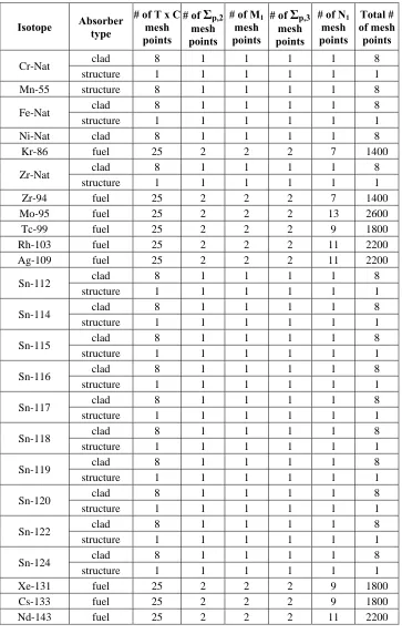
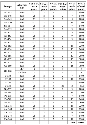
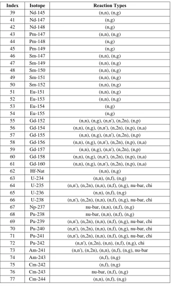
Table 3.2 Cross-sections with quantified covariance data. ... 68 

Table 3.3 Rank and dimension of the self-shielded multi-group cross-section

LIST OF FIGURES

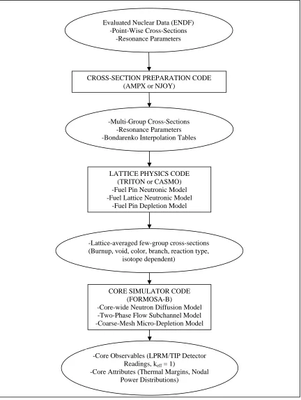
Figure 1-1 Computational sequence for BWR reactor physics design

calculations. ... 15 

Figure 1-2 Detectors Layout (courtesy of Abdel-Khalik). ... 16 

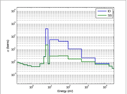
Figure 3-1 U-238 capture cross-section in the resolved resonance energy

range. ... 71 

Figure 3-2 Absolute standard deviation in U-238 multi-group capture

cross-section. ... 72 

Figure 3-3 Relative standard deviation in U-238 multi-group capture

cross-section. ... 73 

Figure 3-4 Lattice k-infinity relative sensitivity coefficient for U-238 capture

multi-group cross-section. ... 74 

Figure 3-5 Singular values for self-shielded multi-group cross-section

covariance matrix. ... 75 

Figure 3-6 Singular values for all covariance matrices. ... 76 

Figure 4-1 Relative standard deviation in lattice k-infinity for a vanished

lattice at 80% void fraction. ... 87 

Figure 4-2 Relative standard deviation in lattice k-infinity for a dominant

lattice at 40% void fraction. ... 88 

Figure 4-3 Relative standard deviation in core k-effective as a function of

Figure 4-4 Absolute standard deviation in relative nodal power profile for a

fresh fuel assembly at BOC. ... 90 

Figure 4-5 Absolute standard deviation in relative nodal power profile for a fresh fuel assembly at MOC. ... 91 

Figure 4-6 Absolute standard deviation in relative nodal power profile for a fresh fuel assembly at EOC. ... 92 

Figure 4-7 Absolute standard deviation in APRAT for a fresh fuel assembly. ... 93 

Figure 4-8 Absolute standard deviation in FLPD margin for a fresh fuel assembly. ... 94 

Figure 4-9 Absolute standard deviation in MFLCPR for limiting CPR fuel assembly as a function of burnup... 95 

Figure 4-10 Prior and posterior error in core k-effective (Case A). ... 96 

Figure 4-11 Prior and posterior core nodal power RMS error (Case A). ... 97 

Figure 4-12 Prior and posterior error in core k-effective (Case B). ... 98 

Figure 4-13 Prior and posterior core nodal power RMS error (Case B). ... 99 

Figure 4-14 Prior and posterior absolute standard deviations in core k-effective (Case B). ... 100 

Figure 4-15 Prior and posterior absolute standard deviations in nodal power (Case B). ... 101 

Figure 4-17 Prior and posterior absolute standard deviations in FLPD margin

(Case B). ... 103 

Figure 4-18 Prior and posterior absolute standard deviations in MFLCPR

margin (Case B). ... 104 

NOMENCLATURE

ACS Adaptive Core Simulation APRM Average Power Range Monitor BOC Beginning-of-Cycle BOL Beginning-of-Life

BP Burnable Poison

BWR Boiling Water Reactor CRP Control Rod Program EOC End-of-Cycle EOL End-of-Life ESM Efficient Subspace Methods

EVD Eigenvalue Decomposition

GPT Generalized Perturbation Theory GWD/MTU Gigawatt-day per metric-tonne-U

LOCA Loss-of-Cooling accident

LP Loading Pattern

LPRM Local Power Range Monitor MOL Middle-of-Life MOC Middle-of-Cycle RM Reich-Moore

1.

Introduction

1.1. Importance of BWR Modeling and Simulation

High-fidelity computational modeling and simulation plays a critical role in the design, licensing, and operation of a nuclear power plant. For Boiling Water Reactors (BWRs), core simulators aid in determining the fuel assembly loading pattern (LP) and control rod program (CRP) over the planned operating horizon of the plant. Likewise, lattice physics codes are used to determine fuel rod loading and the mechanical design of BWR fuel assemblies. In addition to these design-based models, safety analysis codes simulate accident scenarios, such as Loss-of-Cooling-Accidents (LOCA), to set key design limits as part of the plant licensing procedure. Finally, on-line core simulators monitor reactor operation and provide support for the successful control and protection of the power plant. The fidelity of these four computational models impacts the reactor economy through the introduction of design margins (i.e. – distance to design limits) for the fuel assembly and core design. Large model prediction uncertainties increase design margins, which in turn, increases fuel cycle costs and limits the plant’s power rating. On the other hand, decreasing model prediction uncertainties acts to decrease design margins, which beneficially impacts the reactor economy through reducing fuel cycle and/or operating cost or the initial capital investment for a new nuclear power plant.

modeling, and computational uncertainty. Input data uncertainties include uncertainties in basic input data (e.g. - nuclear data) and uncertainties in semi-empirical model parameters (e.g. – drift flux parameters in two-phase flow models). For both basic input data and model parameters, uncertainties are typically due to experimental measurement inaccuracies. In addition to input data uncertainties, modeling uncertainties exist due to either limiting computing resources to model the problem at the fundamental level, or the lack of knowledge of certain physical phenomena (e.g. – semi-empirical modeling). For example, 3-D few-group nodal diffusion methods are used in design-based core simulators as compared to a detailed 3-D multi-group transport model. Finally, computational uncertainties arise from the use of numerical methods to solve the governing system of equations of the computational model. These uncertainties include the effects from floating-point arithmetic error, truncation error, and residual errors associated with matrix-iterative methods employed by BWR computational models.

1.2. Motivation for Research

the adjusted neutron cross-sections in subsequent simulation improves the prediction of core attributes (i.e. – computed metrics such as thermal limits that are not directly measured, but inferred from the values of the core observables). Increasing the fidelity in core attributes predictions is used to a) change the current operating strategy to increase fuel utilization, operating flexibility, or plant power rating, b) increase design freedom for future fuel cycle strategies, c) enhance future BWR plant design, and d) indicate where future experimental efforts should be focused to decrease core attributes uncertainties. This concept of Adaptive Core Simulation (ACS) is the continued focus of this work.

ACS is classified as a discrete inverse problem commonly referred to as a parameter estimation problem or data adjustment problem. These types of problems are closely related to the field of sensitivity and uncertainty analysis. Before the objectives of this work are presented, a summary of previous work on ACS is given. Following the outline of research objectives, previous applications of data adjustment in reactor physics are reviewed along with relevant inverse theory methods and methods of sensitivity and uncertainty analysis. First, an outline of BWR reactor physics design calculations is provided to facilitate the discussion of previous work.

1.3. Overview of BWR Design Calculations

in the resolved resonance energy range and unresolved resonance energy range. This data is processed by a cross-section preparation code (e.g. – AMPX [5] or NJOY [6]) into multi-group cross-section libraries suitable for lattice physics calculations. The energy detail of the multi-group cross-section library depends on the resonance treatment of the lattice physics code, but is typically ~102 energy groups. The lattice physics code uses the multi-group cross-section library to model the time-dependent neutron transport over a 2-D radial slice of a BWR fuel assembly (i.e. - lattice). In the lattice physics calculation, self-shielded multi-group cross-sections are generated for each fuel pin in the fuel assembly based on the fuel pin geometry, the moderator density, and number densities of key resonance-absorbing isotopes. Using the self-shielded multi-group cross-sections, the 2-D multi-group neutron flux distribution is calculated over the fuel lattice. The neutron flux distribution is then used to calculate fission and absorption rates in each fuel pin which are in turn used in a fuel pin depletion model. This series of calculations is repeated over a series of time steps (i.e. - burnup steps) to model the time-dependent neutron transport and nuclide transmutation in a BWR lattice. At each time step, the 2-D multi-group neutron flux is used to generate lattice-averaged few-group cross-sections and in-core detector responses for the core simulator. For BWRs, the few-group cross-section library is functionalized in terms of burnup, moderator void fraction history, fuel color, and branch condition.

transfer model, 3) nuclide depletion model, and possibly 4) semi-empirical fuel performance model. At each time step, the 3-D few-group neutron flux distribution is determined over the entire BWR core. This neutron flux distribution is then used to calculate 3-D power distributions, thermal margins, and other core metrics used by core designers and plant operators to describe reactor performance.

Over the last thirty years, the BWR calculation sequence has reached a stage of maturity in sophistication and applicability with advancements in computing power and resources. This sequence of calculations is not expected to change in the near-term future for advanced BWR reactor designs. Although modeling improvements and refinements are continuous, the fidelity of these models should benefit by using adaptive techniques to reduce input data uncertainty.

1.4. Previous Work on Adaptive Core Simulation

observed that small changes in core observables lead to large changes in the adjusted few-group cross-sections. This ill-posed nature is common among data adjustment problems and generally leads to the use of regularization techniques for robust data adjustment. In [2], Abdel-Khalik introduces the use of Tikhonov regularization [7] to recast the problem into a well-posed one. The Tikhonov regularization parameter is determined experimentally by “trial and error” based on the characteristic L-curve for discrete inverse problems [8]. The few-group cross-section covariance matrix used to constrain the few-group cross-section adjustment was quantified by propagating the multi-group cross-section covariance matrix through the lattice physics calculation.

In the paper by the author, Turinsky, and Abdel-Khalik [9], the few-group cross-section covariance matrix was reevaluated using a refined lattice physics model and a new multi-group cross-section covariance matrix that contained uncertainties to key isotopes such as gadolinium and zirconium that were not provided in the original work. ESM was used to quantify uncertainty in core attributes while minimizing the number of lattice physics calculations and core simulations to 103 and 102, respectively. Few-group cross-section uncertainties were calculated for only one lattice case—that is, a set of burnup dependent group cross-sections for a given fuel color and thermal hydraulic condition. The few-group cross-sections uncertainties for other lattice cases were assumed to be fully correlated to the evaluated lattice case.

burnt-fuel isotope concentrations due to the few-group cross-section adjustment. The sensitivities of core observables with respect to few-group cross-sections from previous fuel cycles were utilized in the plant adaption rather than just a single reload cycle.

1.5. Scope of Research

For this work, it is the author’s goal to develop the capability to adjust multi-group cross-sections used in the lattice physics calculation for BWR ACS rather than few-group cross-sections used in the core simulator calculation. In the ideal case, the cross-section adjustment is performed at the ENDF level so that a wide range of “experiments” are included (e.g. – criticality experimental benchmarks, and plant data from other reactor types). However, this approach is impractical due to the vast amount of evaluated nuclear data and varying degree of cross-section representations. Multi-group cross-section libraries are generally prepared with the end-application in mind, such as light water reactor multi-group section libraries or fast reactor section libraries. Therefore, multi-group cross-section adjustment still allows for plant data from numerous BWR plants to be utilized to increase the robustness of the adaption.

few-group cross-sections were adjusted. This restricted the scope of future fuel cycle optimization to the core level rather than the fuel assembly level, or more specifically the lattice level. In other words, the few-group cross-sections adjusted during plant adaption must be reused in future fuel cycle design. Future fuel cycles must then utilize the same fuel assembly designs as used in previous fuel cycles. Although desirable with regards to equilibrium fuel cycle, this restriction in design freedom opposes recent gains in fuel cycle optimization that introduces multiple fresh fuel assembly designs to the reload cycle [11], and potentially offsets the improvement in model fidelity.

Multi-group cross-section adjustment also influences the mechanical design of the fuel assembly (e.g. - fuel pin radius or fuel pin pitch). However, geometric changes in the fuel assembly influence the unit cell calculations in the lattice physics model. As explained later, the unit cell calculation is modified to propagate resonance parameter uncertainties through the lattice physics calculation. For this work, the use of adjusted multi-group cross-sections for future fuel cycle optimization is only applicable for lattices with the same geometry (e.g. - GE14 10 x 10 lattice designs [12]). Extension of the adjusted multi-group cross-sections to mechanical fuel design optimization is discussed in Section 3.2.

depends on the number of degrees of freedom associated with the multi-group cross-section covariance matrix. In previous work by the author, Abdel-Khalik, and Turinsky [9], N was assumed equal to 1, but is realistically ~103 for current core designs. Since 106 lattice physics calculations are computationally intractable, one of the objectives of this work is to determine the number of active degrees of freedom (i.e. – multi-group cross-sections with high uncertainty and high sensitivity) that are passed through the lattice physics calculation and core simulation. This is performed using both the ESM approach and sensitivity and uncertainty analysis of the lattice physics calculation using generalized perturbation theory (GPT). This approach reduces the number of lattice physics calculations per lattice case by nearly an order of magnitude. For this work, 10 lattice cases are chosen to provide a better understanding of the few-group cross-section uncertainty for the large range of lattice cases required by the core simulator.

Second, core attributes uncertainties due to important resonance parameters’ uncertainties are more accurately quantified. In the previous work on ACS, the multi-group cross-section covariance libraries (44GROUPV5COV and 44GROUPANLCOV [13]) were calculated using the multi-group cross-section preparation code PUFF-III [14].1 PUFF-III calculates multi-group cross-section covariance matrices for resonance-absorbing isotopes using an infinitely-dilute approximation. Therefore, these covariance matrices apply only to infinitely-dilute multi-group cross-sections, and were not previously treated as such. For this work, resonance parameter uncertainties are provided for key resonance-absorbing isotopes

1

(e.g. U-238, Pu-239, Pu-240, Pu-242, Am-241, and Gd isotopes), and their uncertainty contribution is quantified accounting for spatial and energy resonance self-shielding.

Similar to previous work, it is assumed that BWR model prediction uncertainties are dominated by neutron cross-section uncertainties. The uncertainty in key core attributes due to neutron cross-section uncertainty is comparable in magnitude to the observed discrepancies between experimental measurements and plant predictions. Furthermore, the uncertainty quantification calculations using a simplified fuel pin model are comparable in magnitude to the same calculations using the lattice physics model and core simulator. These consistent comparisons validate the claim that neutron cross-section uncertainties dominate the uncertainties due to modeling errors.

1.6. Literature Review

The purpose of this work is to increase the fidelity of BWR computational models through the use measured plant data to adjust multi-group cross-sections. Measured BWR plant data is provided in the form of LPRM and TIP detector readings. For a typical GE BWR/6 reactor core, a string of four LPRM detectors is positioned in the center of four fuel assemblies, in the opposite corner of the control rod blade (see Figure 1-2). The four detectors are positioned at different elevations to monitor the axial power profile. The average of the LPRM signals (i.e. – Average Power Range Monitor (APRM) readings) are displayed in the control room panels and a subset of these readings are input to the reactor protection system. LPRMs are recalibrated every 5 to 6 weeks using TIP measurements [17]. TIP measurements are recorded at 100-150 different axial elevations to recalibrate both the LPRM measurements and the on-line core simulator predictions. A BWR typically uses 4 to 5 TIP machines to service one quarter of the detector channels along with a common channel for calibration. The TIP measurement channels coexist along the LPRM detector strings.

Although current BWR adaption methods are highly proprietary with few published papers, they generally employ similar semi-empirical adjustment techniques verified through operating experience [20]. These approaches differ from the proposed adaptive method of uncertainty-based cross-section adjustment. The proposed approach, formally presented in Section 2.3, requires 1) the sensitivity matrix mapping changes in predicted LPRM readings with respect to changes in multi-group cross-sections, 2) the prior covariance matrices of the multi-group cross-sections and measured LPRM readings2, and 3) the Generalized Linear Least Squares (GLLS) algorithm for cross-section adjustment. Therefore, the proposed adaptive method is rooted in a rigorous mathematical formulation that has been previously applied in other fields of nuclear engineering.

Data adjustment methods have been used extensively for fast reactor design, criticality safety, and reactor shielding. In the 1970s, Weisbin and Marable et al. ([21]-[22]) developed cross-section adjustment methods for fast reactor design in conjunction with the development of the FORSS code system for sensitivity and uncertainty analysis [23]. In [22], measured integral parameters from fast reactor critical benchmark experiments are used to adjust multi-group cross-section libraries used for liquid metal fast breeder reactor design. Covariance data for both the multi-group cross-sections and the integral experiments are used in the data adjustment. Similar to other work on fast reactor analysis [24]-[27] and recent parametric studies for Generation IV reactor concepts by Aliberti et al [28], only a few number of “observables” or integral parameters (e.g. multiplication factor and breeding ratio)

2

are used to consistently adjust a large number of multi-group cross-sections. Because of the small number of observables and that the benchmark experimental system has negligible burnup effects, cross-section sensitivities are calculated using first-order eigenvalue perturbation theory (FOEPT) [29] and generalized perturbation theory (GPT) [30]-[34]. For this work, these methods have limited applicability for three reasons. First, the number of observables (~105 LPRM detector readings) is too large to employ a conventional GPT-based approach. Second, BWR design calculations, as shown in Figure 1-1, are loosely-coupled multi-level nonlinear computational models. Although the theory of adjoint-based sensitivity analysis for nonlinear models is well-developed [35]-[36], it requires considerable effort to “back-fit” existing forward models with linearized first-order adjoint capability. Finally, the computational run-time to determine the first-order adjoint is of the same order as to solve the forward model. In other words, 105 adjoint calculations are just as infeasible as 106 forward calculations in a conventional forward sensitivity study.

and uncertainty analysis as in the best-estimate analysis rather than employ BF and BO approaches.

Figure 1-1 Computational sequence for BWR reactor physics design calculations.

Evaluated Nuclear Data (ENDF) -Point-Wise Cross-Sections

-Resonance Parameters

CROSS-SECTION PREPARATION CODE (AMPX or NJOY)

-Multi-Group Cross-Sections -Resonance Parameters -Bondarenko Interpolation Tables

LATTICE PHYSICS CODE (TRITON or CASMO) -Fuel Pin Neutronic Model -Fuel Lattice Neutronic Model

-Fuel Pin Depletion Model

-Lattice-averaged few-group cross-sections (Burnup, void, color, branch, reaction type,

isotope dependent)

-Core Observables (LPRM/TIP Detector Readings, keff = 1)

-Core Attributes (Thermal Margins, Nodal Power Distributions)

CORE SIMULATOR CODE (FORMOSA-B)

2.

Mathematical Methods for BWR Adaptive Simulation

This chapter outlines the mathematical theory and methods for BWR ACS. The two main methods employed are uncertainty analysis based on first-order sensitivity analysis (i.e. – the “sandwich rule”), and the generalized linear least-squares approach to inverse problems. For this work, these methods are referred to as the uncertainty propagation method and data adjustment method, respectively. A review of the uncertainty propagation method is given in Section 2.2, and the data adjustment method is presented in Section 2.3 based on Tarantola [42]. In each section, the theory of each method is outlined followed by the implementation for BWR ACS.

2.1. Mathematical Notation

The following notation is used consistently throughout this work. Any modified or auxiliary notation is provided in subsequent chapters if needed.

C Matrix. Subscripts are used for descriptiveness (e.g. - CFG - “few-group

cross-section covariance matrix”). Superscripts are used for matrix operations (e.g. -

T FG C or

1

FG

−

C ).

,

i j

C the i-th row and j-th column element of matrix C. Descriptive subscripts are listed before element indices (e.g. CFG i j, , ).

,

i∗

C the i-th row vector of matrix C.

,j

∗

x Vector. Subscripts are used for descriptiveness and superscripts are used for vector operations (e.g. - x_FGT ).

k

x the k-th element of vector x. Descriptive subscripts are listed before the element index (e.g. x_{FG k,} ).

2 , ,b x

α Scalars. Greek letters are reserved for cross-sections unless noted otherwise.

( )

y =Θ x Nonlinear operator. Subscripts are used for descriptiveness. Parentheses are used to list the independent variables that are “mapped” by the operator (e.g. - z =Θ(x y, ) - “operator Θ maps x and y to z”). Nonlinear operators are frequently referred to simply as Θ, where the notation for the domain and range of the operator is suppressed.

,

〈⋅ ⋅〉 Inner product. (e.g. - 〈x y, 〉 =x yT and 〈x y, 〉 =xT y

C C for symmetric, positive definite C).

⋅ Norm. Matrix norms are induced vector norms unless noted otherwise. Subscripts are used in traditional manner (e.g. - ⋅ _p- p-norm and

2

,

x _A = 〈x x〉

A for symmetric, positive definite A). 2-norm is implied unless noted otherwise.

2.2. Uncertainty Propagation

2.2.1.

Theory

parameters uncertainties described by possibly non-Gaussian probability density functions (PDFs). The mathematical expectation of an arbitrary function ( )g x of a vector of continuous input parameters x is given as [44]:

1 2

[ ( )] ( ) ( )

( ) ( )

n

E g x dx dx dx g x f x

dx g x f x

∞ ∞ ∞

−∞ −∞ −∞

∞

−∞ = =

∫

∫

∫

∫

where E g x[ ( )] is the expected value of g x( ) and f x( ) is the multivariate PDF that characterizes the input parameter uncertainty. Introducing the computational model as a nonlinear operator:

( )

y =Θ x (2.2)

where x is an n-th dimensional vector of input parameters, and y is an m-th dimensional vector of observables, then the expected mean and expected covariance of the observables is given as:

[ ] ( ) ( )

1, 2, ,

i i

E y dx x f x

for i m

∞

−∞

= =

∫

, [( [ ])( [ ])]

( ( ) [ ])( ( ) [ ]) ( )

, 1, 2,

i j _{i i j j}

i i j j

E y E y y E y

dx x E y x E y f x

for i j m

∞

−∞

= − −

= − −

=

∫

C

Θ Θ

…

(2.4)

In Eq. (2.3) and Eq. (2.4), Θ( )x _i denotes the i-th observable of the nonlinear operator Θ( )x . The first-order approximation of the computational model is now introduced as:

0 0

( ) ( )

y ≅Θ x +Θ x x− (2.5)

where x₀ stores the mean values of the input parameters and Θ is the model sensitivity matrix, defined as:

0

,

1, 2, ,

1, 2, , i

i j

j x

i m

y for

j n

x

= ∂

=

= ∂

Θ (2.6)

,

0, 0 0,

1 ,

0 0,

1 ,

0 0, 0, 0

1 [ ( ) ( )] ( ) ( ) ( ) ( ) ( ) ( ) ( ) ( ) n i j

i i j j

j n

i j

i j j j j

j n

i j

i j j i

j

y dx x x x f x

x dx f x dx x x f x

x x x x

∞ −∞ ₌ ∞ ∞ −∞ −∞ = = = + − = + − = + − =

∑

∫

∑

∫

∫

∑

0 ( 0)

y x

⇒ =Θ (2.8)

Likewise, the observables covariance matrix C_y is derived as:

, , , _0, , _0,

1 1

, , _{0, 0,}

1 1 , , , , 1 1 [ ( )][ ( )] ( ) ( , )( )( ) n n

y i j i k _{k k} j l _{l l}

k l

n n

i k j l _{k l k l k k l l}

k l

n n

i k j l x l k

k l

dx x x x x f x

dx dx f x x x x x x

∞ −∞ _{= =} ∞ ∞ −∞ −∞ = = = = = − − = − − =

∑

∑

∫

∑ ∑ ∫

∫

∑ ∑

C Θ Θ

Θ Θ

Θ Θ C

(2.9)

T

y x

⇒C =ΘC Θ (2.10)

1) If Θ is linear and the input parameters PDF is Gaussian, then the observables PDF is Gaussian and is fully characterized by y₀ and C_xdetermined by Eq. (2.8) and Eq. (2.10).

2) If Θ is linear and the input parameters PDF is non-Gaussian, then the first and second moments (i.e. mean and covariance) of the observables PDF are determined exactly by Eq. (2.8) and Eq. (2.10). However, y₀ and C_xdo not fully characterize the observables PDF due to the nonzero higher order moments of the input parameters PDF.

3) If Θ is nonlinear and the input parameters PDF is Gaussian, then the first and second moments of the observables PDF are approximately determined by Eq. (2.8) and Eq. (2.10). If Θ has weak nonlinearity effects, then the Gaussian PDF characterized by y₀ and C_x is an accurate approximation of the observables PDF. 4) If Θ is nonlinear and the input parameters PDF is non-Gaussian, then the first and

second moments of the observables PDF are approximately determined by Eq. (2.8) and Eq. (2.10). Further calculations are necessary to determine more accurate first and second moments of the observables PDF and possibly important higher order moments.

that closely approximates the exact core observables PDF assuming that the systematic errors in cross-section measurements are small.

2.2.2.

Implementation

For BWR ACS, the uncertainty propagation method outlined above is used to propagate cross-section covariance data through each stage of the BWR calculation sequence shown in Figure 1-1. Using Eq. (2.10), the following relationships are derived:

T

MG XP ENDF XP

C = S C S (2.11)

T

FG LP MG LP

C = S C S (2.12)

T

CO CS FG CS

C = S C S (2.13)

In Eqs. (2.11)-(2.13), CENDF is the ENDF cross-section covariance matrix, SXP is the

cross-section preparation code sensitivity matrix, CMG is the self-shielded multi-group

cross-section covariance matrix, SLP is the lattice physics sensitivity matrix, CFG is the few-group

cross-section covariance matrix, SCS is the core simulator sensitivity matrix, and CCO is the

that these equations are not used directly because of a) the size of the various matrices, b) the computational burden of each matrix multiplication, and c) the computational burden of evaluating each sensitivity matrix. In addition, conventional forward and adjoint sensitivity methods are not used due to the storage and computational burden of both approaches. For this work, Efficient Subspace Methods are used as developed by Abdel-Khalik in [1].

2.2.3.

ESM Implementation

Efficient Subspace Methods (ESM) calculate accurate low-rank approximations for sensitivity and covariance matrices using singular value decomposition (SVD). ESM only requires the action of the sensitivity matrix operating on a vector (i.e. – matrix-vector product) and possibly the action of the transpose of the sensitivity matrix operating on a vector (i.e. – transpose vector product). One possible method to calculate a matrix-vector product is by the forward perturbation approach. That is, given any matrix-vector q R∈ n and computational model Θ, vector Θq R∈ m is calculated as:

0 0

(x q) (x )

q ε

ε

+ −

≅Θ Θ

Θ (2.14)

where the sensitivities are evaluated at x0. The transpose matrix-vector product for the

sensitivity matrix is referred to as ( )

T p

Throughout this work, the following definitions for singular value decomposition are used from [46]1:

, ( ) ,

m x n rank =r r n m< <

Θ Θ (2.15)

SVD:

T m x n m x n = m x m n x n

Θ U Σ V (2.16)

Thin SVD:

T n x n m x n = m x n n x n

Θ U Σ V (2.17)

Compact SVD:

T r x r m x n = m x r r x n

Θ U Σ V (2.18)

Truncated-SVD:

T T

t xt t

t = m xt t x n = t t

Θ U Σ V U Σ V (2.19)

where the truncated-SVD Θt is rank-t, where t < r, and is the minimizer of

2

min , ( )

t = − for any with rank =t

A

Θ Θ A A A (2.20)

The 2-norm error in Θt is equal to the t+1-singular value of Θ (i.e. - Θt+ +1,t 1). ESM determines the truncated-SVD of Θ provided that the matrix-vector product and the

1

transpose matrix-vector product are available.2 Since the transpose matrix-vector product is unavailable for both the lattices physics model and the core simulator model, the ESM approach utilizes the truncated-SVD of the self-shielded multi-group cross-section covariance matrix to minimize storage and calculation burden. Introducing the truncated-SVD of CMG with t-singular values as:

,

, ,

T MG t

MG ≅ MG t MG t

C U Σ U (2.21)

then the few-group cross-section covariance matrix CFG is given as (cf. - Eq. (2.12)):

,

, ,

T

FG LP MG LP

T T

MG t

LP MG t MG t LP

=

≅

C S C S

S U Σ U S

(2.22)

1/ 2 1/ 2

, ,

, ,

, ,

( MG t)( MG t)T

FG LP MG t LP MG t

T LP t LP t =

=

C S U Σ S U Σ

R R

(2.23)

Using this approach, CFG is calculated with t matrix-vector products of SLP (i.e. - 1/ 2

, ,

( MG t)

LP MG t

S U Σ ). The matrix RLP t, denotes the matrix storage of the t matrix-vector

2

products. Since there are ~106 few-group cross-sections, the matrix-matrix multiplication

, ,

T LP t LP t

R R is impractical. However, important elements of CFG (e.g. – diagonal elements),

are calculated by:

, ,

, , ,

1

i k j k i j

t

LP t LP t FG

k= =

∑

C R R (2.24)

The matrix RLP t, is directly used to calculate the core observables covariance matrix.

Given the truncated-SVD of RLP t, with rank-t2, which is less than rank-t:

2 2

2

, , , ,

T LP t ≅ LP t LP t LP t

R U Σ Ψ (2.25)

then CCO is calculated as (cf. - Eq. (2.13)):

, ,

T

CO CS FG CS

T T

LP t LP t

CS CS

=

=

C S C S

S R R S

(2.26)

2 2 2 2

2 2 2 2 , , , , , , , , ( ) ( ) T _T

LP t LP t LP t LP t

CO CS LP t CS LP t

T CS t CS t =

=

C S U Σ Ψ Ψ S U Σ

R R

In Eq. (2.27), CCO is calculated with t2 matrix-vector products of SCS. Since the right

singular vectors ΨLP t,2 are not needed in Eq. (2.27) (i.e. - ,2 ,2

T

LP t LP t =

Ψ Ψ I), matrix RCS t,2

stores only SCS(ULP t,2ΣLP t,2). However, ΨLP t,2 is needed for data adjustment and is

explained in Section 2.3.2. Important elements of CCO are calculated by:

2

2 , 2 ,

, , ,

1

i k j k i j

t

CS t CS t CO

k=

=

∑

C R R (2.28)

In summary, the ESM approach of uncertainty propagation for BWR ACS requires 1) the calculation of the truncated-SVD of CMG, 2) the selection of rank-t, 3) t-matrix vector

products of SLP, 4) the truncated-SVD of RLP t, , 5) the selection of rank-t2, and 6) t2

matrix-vector products of SCS. These steps are outlined in more detail in Chapter 3.

2.3. Data Adjustment

2.3.1.

Theory

The data adjustment method for BWR ACS follows the generalized linear least-square approach given in [42]. The following information about the input parameters and observables is given a priori:

0

x

C prior input parameters covariance matrix

m

y prior observables (i.e. - measured observables)

m

y

C prior observables covariance matrix (i.e. - the uncertainty in the measured observables).

( )

y =Θ x the computational model

The goal is to adjust x₀ to a new value, denoted x, that minimizes3:

2 2

1

1 ₀

min{ ( ) }

m

m _x

x y

x= y − x − + x x− _C−

C

Θ (2.29)

Using the first-order approximation to the nonlinear computational model Θ:

0 ( 0)

y≅ y +Θ x x− (2.30)

then Eq. (2.29) becomes:

2

2 1

0 0 1 0

min{ ( ) }

m

m _x

x _y

x = y −y − x x− ₋ + x x− −

C C

Θ (2.31)

3

The solution to Eq. (2.31) is given in [42] as:

1 1 1

0 0

0 0

1 1

1

1

( ) ( )

( ) ( )

( )

m m

m

T T

y x y _m

T

x y x

T

y x

x x y y

y x y x x

− − −

− −

−

−

= + + −

= ≅ + −

= +

=

Θ C Θ C Θ C

Θ Θ

C Θ C Θ C

C ΘC Θ

(2.32)

where x is the posterior input parameters, y is the posterior observables, Cx is the posterior

input parameters covariance matrix, and Cy is the posterior observables covariance matrix.

The posterior values in Eq. (2.32) are determined by the normal equation solution of the generalized linear least-squares equation.

2.3.2.

ESM Implementation

For BWR ACS, the goal is to adjust the set of self-shielded multi-group cross-sections to minimize the disagreement between measured core observables and predicted core observables. The following information is given a priori:

0 MG

x prior self-shielded multi-group cross-sections

0 FG

x prior lattice-averaged few-group cross-sections

MG

C prior self-shielded multi-group cross-sections covariance matrix

m

CO

m

CO

C prior core observables covariance matrix (i.e. - the uncertainty in the measurements of core observables).

LP

Θ lattice physics computational model

CS

Θ core simulator computational model

0 CO

y prior core observables as predicted by computational model

n dimension of

0 MG

x (~107)

m dimension of

m

CO

y (~105)

The first-order approximation to the computational model is given as:

0 CS LP( 0)

CO CO MG MG

y = y +S S x −x (2.33)

where SLP and SCS are the sensitivity matrices of the lattice physics model and core

simulator model respectively. The data adjustment problem is now given as (cf. – Eq. (2.31)):

0 0 0

2 ₂

1 1

min{ ( ) }

m MG

m

CS LP

MG _x CO CO MG MG MG MG _MG

CO

x = y −y − x −x ₋ + x −x −

C C

S S (2.34)

where x_MG is the posterior self-shielded multi-group cross-sections. Eq. (2.34) represents an ill-posed data adjustment problem for the following two reasons. First, the prior self-shielded multi-group cross-sections covariance matrix CMG is replaced by its truncated-SVD (i.e. -

,

, ,

T MG t

MG t MG t

U Σ U ), so

1

MG

−

0 0

†

(x_MG−x_MG )TC_MG(x_MG−x_MG ), where the Moore-Penrose pseudoinverse matrix of CMG has

been introduced (i.e. -

† 1

,

, ,

T MG t

MG MG t MG t

−

C U Σ U ). Introducing the pseudoinverse of CMG leads

to an infinite number of possible solutions for the data adjustment problem. To ensure that the least-squares solution is unique (i.e. – well-posed), the self-shielded multi-group cross-section adjustment is constrained to the subspace spanned by the t singular vectors of U_{MG t,} .

Second, SLP and SCS are ill-conditioned (i.e. – small singular values) and

m

CO

y contains inherent noise that is several orders of magnitude larger than the small singular values associated with the ill-conditioned sensitivity matrices. This can lead to unphysical cross-section adjustments along singular vectors corresponding to the small singular values of the sensitivity matrices. Regularization techniques need to be employed to recast the ill-conditioned, ill-posed data adjustment problem into a well-posed one..

For BWR ACS, the following modifications are made to Eq. (2.34) to produce a well-posed data adjustment problem:

0 0 0 0

0 0 0 2 , † †

min{[ ( )] [ ( )]

( ) ( )}

( )

MG

T

CS LP CS LP

MG _x CO CO MG MG CO CO MG MG

MG MG MG MG

MG t MG MG COm m m MG T

x y y x x y y x x

x x x x

subject to x x R

α

= − − − − − − +

− −

− ∈

S S C S S

C

U

(2.35)

as the misfit chi-square χ_m2, and the second term is referred to as the regularization

chi-square 2

r

χ . The n by n matrix 1

m

CO

−

C is replaced with its pseudoinverse †

m

CO

C by introducing the following compact SVD of the prior core observables covariance matrix:4

† 1

m m m m

m m m m

T CO

CO CO CO

T CO

CO CO CO

− =

=

C U Σ U

C U Σ U

(2.36)

Because the self-shielded multi-group cross-section adjustment

0

MG MG

x −x is constrained to

, ( MG t)

R U , the following change in variables is introduced:

0

1/ 2

, ,( )

T

MG MG t MG t MG MG

z =Σ− U x −x (2.37)

0

1/ 2 , ,

MG MG MG t MG t MG

x =x +U Σ z (2.38)

where z_MG is defined as the data adjustment vector. From Eq.(2.37), the j-th element of vector z_MG represents the magnitude of self-shielded multi-group cross-section adjustment

along the j-th singular vector of UMG t, , divided by the square root of the j-th singular value.

4

m

CO

C is treated as a diagonal matrix. With real plant data, CCOm is expected to be block diagonal, with each

The physical interpretation of this change in variables is explained in the following example. Suppose that CMG is a diagonal matrix where the diagonal elements represent the variance of

each self-shielded multi-group cross-section. The j-th singular vector of CMG is the standard

basis vector e_j and the j-th singular value is the variance of the j-th self-shielded multi-group cross-section. Eq. (2.37) and Eq. (2.38) become:

0 0 0 0 , , , , , 1 , ( ) ( )

MG j MG j

MG j j MG MG

MG j MG j

x x

z e x x

SD x SD x

−

= 〈 − 〉 = (2.39)

0 0

, , ( , ) ,

MG j MG j MG j MG j

x =x +SD x z (2.40)

where

0,

( _{MG j})

SD x is the standard deviation in the j-th self-shielded multi-group cross-section. Eq. (2.40) states that if z_{MG j,} equals one, then the j-th self-shielded multi-group cross-section is adjusted by one standard deviation. In the general case of Eq. (2.37), z_{MG j,} represents the number of “standard deviations” the self-shielded multi-group cross-sections are adjusted along the orthornomal direction specified by the j-th singular vector of CMG. Because of the

truncated-SVD representation of CMG, the dimension of z_MG is only t as compared to n in

the above example. Using this change in variables, Eq. (2.35) reduces to:

0

2

1/ 2 1/ 2

1/ 2

2

( )

min{ }

0

m m t m m _m

MG

T T

CO CO CS LP MG MG

CO CO _{CO CO}

MG _z MG

y y z z α − − ⎡ ⎤ ⎡ ₋ ⎤ ⎢ ⎥ ⎢ ⎥ = − ⎢ ⎥ ⎢ ⎥ ⎣ ⎦ ⎣ ⎦

Σ U S S U Σ

Σ U

I

where z_MG is the posterior data adjustment vector. The approach to solving Eq. (2.41) builds

upon the ESM solution method for uncertainty propagation. Using matrices ΨLP t,2 and

2

, T CS t

R from Section 2.2.3, the following thin SVD is defined:

2 2 3 3 3

1/ 2 , , 3 3 3 3 3 2 m m

T T T

CO CO CS t LP t t t t

T is n t

is t t

is t t

t t t

− = × × × ≤ ≤

Σ U R Ψ U Σ V

U

Σ

V

(2.42)

Using the thin SVD in Eq. (2.42), it is shown in Appendix A that the solution to Eq. (2.41) is the following (cf. - Eq. (2.32)):5

0

0

0

2 2

0

2 1/ 2

2 1 1/ 2 , , , , ,

1/ 2 2 2 1/ 2

2 2 4

, , , , , ( ) ( ) ( ) ( ( )) ( ) ( )

m m _m

T T

CO CO

MG CO CO

MG t MG t

MG MG MG

LP t

FG LP MG FG MG

T CS t LP t

CO CS LP MG CO MG

T T

MG t MG t

MG post MG t MG t

F

z y y

x x z

x x x z

y x y z

α α α − − − = + − = + = ≅ + = ≅ + = + +

V Σ I ΣU Σ U

U Σ

Θ R

Θ Θ R Ψ

C U Σ V Σ I Σ I V Σ U

C

2 2 2 2

2 2

2 2 4

, ,

,

2 2

2 2 4

, , , ,

,

( ) ( )

( ) ( )

T T

LP t LP t

G post

T T T

CS t LP t LP t CS t

CO post α α α α − − = + + = + +

R V Σ I Σ I V R

C R Ψ V Σ I Σ I V Ψ R

(2.43)

5

In this formulation, the Tikhonov regularization parameter is assumed be nonzero. If the Tikhonov regularization parameter is zero, the matrix

2

2 1

(Σ +α I)− is replaced by the pseudoinverse 2

where x_MG is the posterior self-shielded multi-group cross-sections, x_FG is the posterior

3.

Cross-Section Uncertainty Propagation

In this section, the uncertainty propagation calculations outlined in Chapter 2 are now described in more detail. These calculations involve 1) propagating ENDF cross-section covariance data to calculate the self-shielded multi-group cross-section covariance matrix, 2) propagating the self-shielded multi-group cross-section covariance matrix through the lattice physics model TRITON, and 3) propagating the few-group cross-section covariance matrix through the core-simulator model FORMOSA-B [47]. In step 1), PUFF-IV processes the ENDF covariance files to calculate an infinitely-dilute multi-group cross-section covariance matrix. Additional calculations are necessary to quantify the uncertainty in self-shielded multi-group cross-sections used in the lattice physics calculation. To perform these calculations, the resonance treatment model in TRITON was modified to quantify this uncertainty contribution due to spatial and energy resonance self-shielding effects for each fuel pin. In Section 3.1, the modified resonance self-shielding model is presented and the uncertainty propagation calculations are described.

physics sensitivity matrix on the self-shielded multi-group cross-section covariance matrix. This GPT-based approach is used to reduce the number of lattice physics forward perturbations calculations to 481 per lattice case. These calculations are summarized in Section 3.2.

As a result of the calculations described in Section 3.2, the truncated-rank of the few-group cross-section covariance matrix is 362. This implies that 362 core simulator forward perturbation calculations are necessary to calculate the core observables covariance matrix. The analysis of these calculations for a BWR/4 reload core design is deferred to Chapter 4.

3.1. Multi-Group Cross-Section Covariance Matrix

3.1.1.

PUFF-IV Methodology

Quantifying multi-group cross-section uncertainty due to ENDF cross-section uncertainty constitutes a major contribution to BWR ACS in this work. Repeating from Chapter 2, this calculation is given as:

T

MG XP ENDF XP

C = S C S (3.1)

where CENDF is the ENDF cross-section covariance matrix, SXP is the cross-section

preparation code sensitivity matrix, and CMG is the self-shielded multi-group cross-section

in the resolved resonance energy range, 3) point-wise cross-section covariance data, and 4) the resonance parameter covariance data. The point-wise cross-section data are represented in vector form as σ_PW where each element corresponds to a unique point-wise cross-section for a given reaction type and isotope at a specific neutron kinetic energy. Similarly, the point-wise cross-section covariance data is represented in matrix form as CPW. Since

cross-sections for each isotope are measured independently (with the possible exception of ratio measurements to determine fission cross-sections), CPW is sparse, block diagonal in

structure with each diagonal block corresponding to a given isotope. Likewise, the resonance parameter data is represented as x_RP and CRP. Combining the covariance data from both of

these matrices, CENDF is given as:

0 0

PW ENDF

RP

⎡ ⎤

⎢ ⎥

=

⎢ ⎥

⎣ ⎦

C C

C (3.2)

Although CPW and CRP are represented as uncorrelated in Eq. (3.2), each matrix

cross-section resonances in the neighborhood of an individual resonance. Combining the long-range and short-long-range covariance components by Eq. (3.2) completely describes the cross-section uncertainty over the full cross-cross-section energy range.

Cross-section preparation codes generate multi-group cross-sections by 1) constructing the neutron cross-section component described by the resonance parameters over an ultra-fine energy mesh (i.e. - ~105 energy grid points), 2) adding the resonance parameter cross-section component to the point-wise cross-section component, and 3) homogenizing the combined cross-section using an ultra-fine neutron flux spectra. This calculation is represented by the following:

( ( ))

ID ID PW xRP

σ =H Pσ +Π (3.3)

where σ_ID is the multi-group cross-section vector, HID is the energy-averaging

homogenization operator, P is a prolongation operator the maps σ_PW from the ENDF point-wise energy mesh to the ultra-fine energy mesh, and Π is the nonlinear operator that maps cross-section resonance parameters to cross-section values on the ultra-fine energy mesh.

0

0

T

PW PW

ID PW RP

T

RP _RP

T T

PW PW PW RP RP RP T LR RP RP RP

⎡ ⎤

⎡ ⎤

⎡ ⎤_{⎢ ⎥}⎢ ⎥

= ⎢_⎣ ⎥_{⎦⎢ ⎥⎢ ⎥}

⎣ _{⎦ ⎣ ⎦}

= +

= +

C S

C S S

C _S

S C S S C S

C S C S

(3.4)

where SPW =H PID and SRP =HIDΠ. PUFF-IV has many options to analytically calculate

the sensitivity matrix Π for the nonlinear operator Π evaluated at the prior mean values of the resonance parameters. In the last expression in Eq. (3.4), the matrix CLR is used to

represent

T PW PW PW

S C S . This matrix represents the long-range uncertainty contribution to the multi-group section covariance matrix as well as the uncertainties in multi-group cross-sections for energy ranges above and below the resolved resonance energy region.

PUFF-IV was used to calculate the 44GROUPV6REC multi-group cross-section covariance file that is used for this work. A complete description of 44GROUPV6REC is given in [48]. In generating the 44GROUPV6REC covariance file, a 1/E neutron flux spectrum was used to homogenize the ultra-fine cross-sections. The subscript “ID” in σ_ID,

ID

H , and CID is used to denote the infinitely-dilute approximation used in generating

multi-group cross-section covariance matrices. It is well known that infinitely-dilute multi-multi-group cross-sections can differ with multi-group cross-sections that account for spatial and energy resonance self-shielding by several orders of magnitude. Consequently, the self-shielded multi-group cross-section covariance matrix CMG can differ from CID. Unfortunately, the

self-shielding effects for each fuel pin depends on local thermal hydraulic conditions and fuel pin number densities. It is computationally infeasible to calculate CMG for each fuel pin at each

burnup step for each lattice case using problem-dependent self-shielded neutron flux spectra. In the following section, the Nordheim Integral Treatment is presented to calculate CMG for

a single unit cell (i.e. - fuel pin/clad/coolant “unit” used to construct the lattice). The modified resonance self-shielding model presented in Section 3.1.3 is used to consistently perturb the self-shielded multi-group cross-sections for any unit cell in the lattice physics uncertainty calculations.

3.1.2.

Nordheim Integral Treatment

In the Nordheim Integral Treatment Method presented in the NITAWL code manual [49], the unit cell is represented by two spatial regions: the absorber region containing the resonance absorber (i.e. – resonance-absorbing isotope) and the external moderator region. By using first-flight escape probabilities to describe the neutron transport into and out of each region, as well as the reciprocity relationship between the first-flight escape probabilities in these two regions, the following equation can be shown to describe the energy-dependent neutron flux in the absorber region over a given cross-section resonance1:

/(1 ) 3

,

* *

0 0

1

( ', ) ( ', )

( , ) ( , ) (1 ( , )) ' ( , ) ( , ) ( )

'

j

E

s j

t t

j _E

E T E T

E T E T P E T dE P E T E T W E

E

α _φ

φ

−

=

Σ

Σ = −

∑ ∫

1

where ( , )φ E T is the self-shielded neutron flux over the cross-section resonance energy range, ( , )Σ_t E T is the total macroscopic cross-section of the absorber region, P E T₀*( , ) is the Dancoff-corrected escape probability of the absorber region, Σ_{s j,} ( , )E T is the macroscopic scattering cross-section of mixture-j in the absorber region, W(E) is the neutron slowing-down source in the external moderator region, and α_j is the parameter used to describe the neutron energy loss due to elastic scattering. In this formulation, α_j is equal to 4Aj/(Aj+1)2,

where Aj is the effective nuclide mass of mixture-j. (Note that this definition of alpha is

actually 1 minus alpha in many sources [49].) The temperature dependence is explicitly shown in the variables above to indicate the use of Doppler-broadened cross-sections.

Eq. (3.5) is referred to as the Nordheim Integral Equation, and is used to determine the self-shielded neutron flux for both clad-region resonance absorbers and fuel-region resonance absorbers. For clad-region resonance absorbers, the absorber region in Eq. (3.5) is the clad volume and the external moderator region is the fuel and coolant volume. Likewise for fuel-region resonance absorbers, the absorber region is the fuel volume and the external moderator is the clad and coolant volume. Once the self-shielded neutron flux is determined for all cross-section resonances for a given resonance absorber, the self-shielded multi-group cross-sections for that resonance absorber are determined by the following equations:

, , , ,ref , ,

shielded

x g T x g T x g T

σ ₌σ∞ _{+ Δ}