Division V
DAMAGE EVALUATION AND INTEGRITY ASSESSMENT FOR
STRUCTURES UNDER IMPACT LOADINGS
Jiansong Guo
Seismic SQEP, Civil Design Group, Plant Engineering Branch, EDF Energy, UK
ABSTRACT
In the modern Nuclear Power Plants (NPP) design, it is essential and a fundamental requirement for any nuclear safety related structure and system to be seismically qualified. This could bring a significant advantage and provide a critical reference to the nuclear safety engineers in their assessment works for the scenarios associated with the structures or systems under impact loadings.
This paper presents the detailed assessment procedures suggesting a general approach for the assessment of impact induced damage to a structure or system by evaluating the structural response against the existing seismic solution which have been developed in the design assessment stage. It is on the basis of a postulated fault condition, firstly using DANY-Tool to derive the Dynamic Amplification Factor (DAF) and then followed by a detailed analytical analysis demonstrating the feasibility of this general approach.
The paper is concentrated on analysis methods and techniques. The assessment is based on a postulated fault condition. During this fault event, the deceleration of the structure/system would induce a significant impact loading. The integrity of the structure/system under this deceleration impact loading is assessed by demonstrating the structural response due to the impact hazard being enveloped by that due to the frequent and infrequent seismic events, i.e. 10-3 p.a. and 10-4 p.a.
INTRODUCTION
It is essential and a fundamental requirement for any nuclear safety related structure and system to be seismically qualified in the modern Nuclear Power Plants (NPP) design. This could bring a significant advantage and provide a critical reference to the nuclear safety engineers in their assessment works for the scenarios associated with the structures or systems under impact loadings.
The objective of this paper is to provide an assessment methodology for seismic qualified structures subjected to in service impact loading through a postulated fault scenario. For nuclear security reasons, the scenario and assumptions presented in this paper are hypothesized and simplified. They may not be appropriate for direct use in practice.
The presentation is through an example where a postulated fault condition is assumed for a machine having equipment transportation functions during operations. During this fault event, the deceleration of the machine would induce a significant impact loading. The integrity of the machine under this deceleration impact loading is assessed by demonstrating the structural response due to the impact hazard being enveloped by that due to the frequent and infrequent seismic events.
POSTULATED SCENARIO AND ASSUMPTIONS
speed of machine, end of travel limit switches which cut power to the motors and apply the brakes, and profiled end stops which are intended to stop the machine in a controlled fashion.
The fault scenario assumed in this paper is that a transportation machine can go into an overspeed condition during its travel, exceeds its normal travel limits without being stopped by operators or the limit switches.
The derivation of the acceleration-time history during the fault condition is dependent on variety of parameters: the traction force, the rolling resistance, angles of slopes and the application of brake, etc. Note this is not the objective of this paper. However, in order to concentrate on the objective of this paper the derivation of the acceleration-time history has been simplified in which the traction force due to driving wheels, the rolling resistance, and the angle of slope (only one angle is considered) are assumed constant. And only one travelling direction was assumed and presented.
On the basis of the assumptions above, the following key relevant results to this paper can be obtained:
• The max deceleration = 0.317m/s2
• The max speed (v) = 0.152 m/s
The values above are significantly higher than these employed in the original design.
If the final speed (u) is assumed to be 0 m/s, and using v=u + at, the time of the deceleration acting on the machine will be t = 0.48 s, via t = (0.152 - 0)/0.317. Note that the speed value used here is the maximum overspeed instead of the normal speed which is less than 0.152 m/s.
Note that the slope will cause the two driving wheels upon it to slip and prevent forward motion. In consequence, overshooting the end stops will not occur.
ANALYSES
Calculation using DynaTool Software
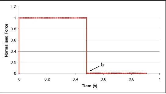
On the basis of the above, the acceleration – time history would be in a rectangular shape with a constant acceleration value of 0.0323g over a duration of acting time of 0.48 s. The normalised acceleration time history is presented in Figure 1. This impact dynamic load produces different effects from a static load. The response of the structure subjected to the impact loading is a function not only of the position and characteristics of the structure, but also of the time during which the force acts on the structure.
0 0.2 0.4 0.6 0.8 1 1.2
0 0.2 0.4 0.6 0.8 1
Tiem (s)
N
o
rm
a
li
s
e
d
F
o
rc
e
td
A dynamic load can have a significantly larger effect than a static load of the same magnitude due to the structure's inability to respond quickly to the loading (by deflecting). The increase in the effect of a dynamic load is given by the dynamic amplification factor (DAF), defined as the ratio of the dynamic displacement to the static displacement.
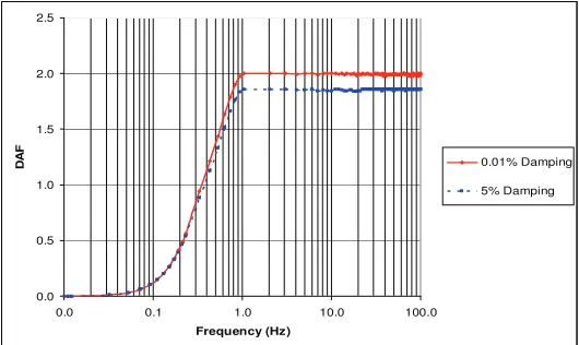
In order to derive the dynamic amplification factor representing the dynamic responses of the machine end-stop collision, DynaTool (Ref 1) was chosen to be employed in the analysis for the scenario interested. The pre-specified acceleration - time history, as presented in Figure 1, has been used as ‘input’ to the calculation. Two different levels of damping have been considered namely: 0.01% representing no-damping, and 5% representing damping for normal structures. Note Reference 2 indicates 5% damping is conservative as the damping level for the machine is in the range from 5% to 10%.
The result from DynaTool is presented in Figure 2. It can be seen that (1) for an undamped system, the maximum DAF can reach up to two, (2) the DAF gradually increases to its maximum value of 2 for frequency in the range from zero to 1 Hz approximately, (3) the DAF remains the maximum constant value of 2 through the whole range of frequency higher than 1 Hz (not a function of frequency), and (4) for damping ratio = 5% the maximum DAF is approximately equal to 1.85.
0.0 0.5 1.0 1.5 2.0 2.5
0.0 0.1 1.0 10.0 100.0
Frequency (Hz)
D
A
F
0.01% Damping
5% Damping
Figure 2, Dynamic Amplification Factor obtained using DynaTool Program
Calculation using Analytical Approach
To prove the program obtained DAF above is correct, an analytical explanation for the derivation of the DAF is presented in the followings (Refs 3 -5).
For a single degree of freedom system, subject to random dynamic force (F1(t)), with stiffness k, mass m and damping constant c, the equation of motion can be expressed as:
)]
(
[
1f
t
F
y
c
ky
y
m
+
+
=
(1)Where y is the displacement, F1 is a constant force value which may be arbitrarily chosen, and f(t) is a non-dimensional time function.
Equation (1) can be simplified to
)] ( [ 1
2 2 F1 f t m
y y
y+
ξω
+ω
=Where
m
k
=
ω
is the angular frequency of the system, andω
ξ
m c
2
= is the damping ratio. If we
assume the angular frequency of a damped system
ω
' (ω
'
=
1
−
ξ
2ω
) equals to that for the un-dampedsystem, the solution (homogeneous solution) for equation (2) with
F
1[
f
(
t
)]
= 0 can be given as:t
e
A
t
e
A
t
y
ξωtω
ξωtω
cos
sin
)
(
=
1 −+
2 − (3)Where A1 and A2 are constants and can be determined by using initial condition: when t = 0, y = y0, and
0
y
y
=
. We have:ω
ξω
0 0 1 y yA = + , and
A
2=
y
0. Substitute to equation (3), the homogeneoussolution details as:
t e y y t e y t
y t t
ω
ω
ξω
ω
ξω ξω sin cos )( 0 0
0
−
− +
+
= (4)
To obtain the general solution of (2), we also need to derive the specific solution. For doing this, we consider the concept of impulse, which is defined as the area under the load-time curve.
For a constant force F1 acting on a system for a duration of ∆t, the impulse is
F
1∆
t
. According to momentum law we have:F
1dt
=
mv
−
mv
0. Before the impulse loading the system is assumed to be atrest (both displacement and velocity are equal to zero,
v
0=
u
0=
0
). After the impulse the system gains avelocity (
m dt F
v= 1
), but the displacement is still zero. Thus, the displacement at time t due to the single
element impulse load will be: e t m dt F t
ω
ω
ξω sin1 − . Therefore, for a general impulse loading
[
(
)]
1
f
t
F
,the total displacement at time t can be obtained by performing integration of the effects of all elements of impulse between zero to t, which gives:
³
− = − − t t d t e f F m y 0 ) (1[ ( )] sin ( )
1
ˆ
τ
ω
τ
τ
ω
τ
ξω (5)
Equation (5) is the specific solution of equation (2). The combination of the homogeneous solution (equation (4)) and the specific solution (equation (5)) forms the general solution to equation (2). If we
conservatively ignore the damping effects, and note the fact that
m F k F
yst 1 21
ω
== , the general solution
to equation (2) can be simplified to:
³
−+ +
=
t
st f t d
y t y t y t y 0 0
0cos sin ( )sin ( )
)
(
ω
ω
τ
ω
τ
τ
ω
ω
(6)The combination of first two terms in the above equation represents the behaviour for un-damped free vibration system. The third term characterises un-damped forced vibration system.
0
)
0
(
=
y
, together withy
(
0
)
=
0
and , this results in the dynamic response for this particular case being the following formula:) cos 1 ( )
( 1 t
k F t
y = −
ω
(7)Now, we consider a force, with load-time history in a rectangular shape, acting on an un-damped system, which is the scenario we are interested in. The system starts at rest and up to time td (td = 0.48 s, as seen in Figure 1), equation (7) applies, and at the time of td we have:
) cos 1 ( 1 d d t t k F
y = −
ω
(8)and its differentiation form will be:
d d
t t
k F
y = 1
ω
sinω
(9)When t is greater than td, the response of the system can be determined by applying equation (7). Noting the initial conditions and the fact of f(t) = 0, we have:
]
cos
)
(
[cos
)
(
sin
sin
)
(
cos
)
cos
1
(
1 1 1t
t
t
k
F
t
t
t
k
F
t
t
t
k
F
y
d d d d dω
ω
ω
ω
ω
ω
−
−
=
−
+
−
−
=
(10)Noting that the dynamic amplification factor
µ
equals to the ratio of dynamic displacement to staticdisplacement (
st
y
y
=
µ
), and the static displacement yst beingk F yst
1
= , we have:
T t
t
π
ω
µ
=1−cos =1−cos2 , fort
≤
t
d (11)T t T t T t t t t d
d
ω
π
π
ω
µ
=cos ( − )−cos =cos2 ( − )−cos2 , fort
≥
t
d (12)Differentiating equations (11) and (12) with respect to time t, and let them equal to zero to obtain the time (tm) of maximum response (or maximum dynamic amplification factor), and substituting the value of tm to equations (11) and (12), the maximum dynamic amplification factor can be obtained.
Alternatively, by careful inspection of equations (11) and (12), it may be found that when 2
T t = ,
equation (11) has its maximum value, and it equals to 2. For equation (12), it can be found that the
maximum value occurs when = =0.5
T t T
t d
, and its value is also equal to 2. Therefore, the maximum
STRUCTURAL INTEGRITY ASSESSMENT OF THE MACHINE
The machine has been seismically qualified at both frequent and infrequent seismic events in the original design process. The infrequent event and the frequent event corresponds to the bottom line and second line cases respectively. For the bottom line case the spectra are site specific Uniform Risk Spectra expected values with a probability of exceedance of 10-4 pa. The peak ground accelerations are 0.21g horizontally and 0.14g vertically. The ground motion used for the second line case is defined by the UK soft site 0.1g PML spectra. The peak ground accelerations are 0.10g horizontally and 0.07 vertically. The ground motion specification with respect to the Bottom Line and Second Line for this nuclear plant is presented in Figure 3. The other two lines presented in the same figure will be interpreted and discussed in the following sections.
The seismic qualification performed in the original design has concluded the structure/system/components of the machine are not compromised by the frequent and infrequent seismic events.
From analyses presented in section - Analysis, it can be concluded that the maximum DAF is a function of the ratio of dynamic load duration to natural period (
t
dT
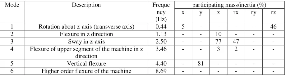
). The natural period of the machine has been derived in Reference 2. The machine vibration testing was performed to monitor the vibration of the machine as it moved in its travel direction. Testing was conducted at a total of five locations, namely: Position 1 to 5. Based on the measured test data, the natural frequencies at the five locations were calculated, which are reproduced in Table 1.The first six modes of vibration for the machine were derived by using ABAQUS finite element analysis (Ref. 2), which are reproduced in Table 2.
It can be seen from Table 1 that the first and second response frequencies for all the measured locations, except for Position 3, are less than 1 Hz. This implies that the DAF could be less than the maximum value of 2. Even for the third response, the corresponding frequencies are only slightly higher than the critical value of 1 Hz. Table 2 also shows that the frequency value of the first fundamental mode is below 1 Hz, again indicating the DAF for this mode can not reach the peak DAF value.
Table 1Calculated Frequencies (Hz) at five Locations of the Machine (Ref. 2)
Position 1 Position 2 Position 3 Position 4 Position 5 1st Response
Frequency (Hz)
0.57 0.53 0.53 0.63 0.54
2nd Response Frequency (Hz)
0.87 0.62 1.13 0.86 0.89
3rd Response Frequency (Hz)
1.14 1.20 1.27 1.17
Table 2Vibration Modes of the Machine Derived using ABAQUS (Ref. 2)
participating mass/inertia (%)
Mode Description Freque
ncy (Hz)
x y z rx ry rz
1 Rotation about z-axis (transverse axis) 0.44 5 - - - - 46
2 Flexure in z direction 1.13 - - 10 - - -
3 Sway in z-axis 2.50 - - 77 47 - -
4 Flexure of upper segment of the machine in z direction
3.46 - - 3 2 - -
5 Vertical flexure 4.40 - 81 - - - -
‘-‘ indicates a participating mass/inertia less than 1%.
Figure 3 presents comparison of the spectral accelerations associated with Bottom Line, Second Line and the Impact Line, over frequencies from 0.3 Hz to 40 Hz. The Impact Line is defined as the multiple of the acceleration and the DAF (labeled as Acc x DAF in Figure 3). The line in the range from 0.3 Hz to 1 Hz for the Bottom Line is extrapolated on the basis of retaining the same shape as the Second Line in the corresponding frequency regime. By inspection of Figure 3 in line with the vibration modes and corresponding frequencies presented in Tables 1 and 2, the following observations can be made:
• The Bottom Line bounds the Impact Line for all frequencies higher than 0.415 Hz. This covers all possible vibration modes for the machine. No frequency is less than this value (0.415 Hz) for the machine investigated.
• For frequency higher than 0.532 Hz, both the Second Line and the Bottom Line envelope the Impact Line.
• For frequencies between 0.415 Hz and 0.532 Hz, the Second Line does not bound the Impact Line, however, the Bottom Line does.
• The lowest frequency of the machine (0.44 Hz in Table 2), is marginally lower than 0.532 Hz. However, it corresponds to rotating vibration mode. The participating mass factor is significantly low (~ 5%) in the transverse directions. Considering the fact that the impact load investigated can only generate transverse vibration, this mode will not be significantly excited in the impact scenario, so it is expected that the overall response will still be enveloped by the response to the second line seismic motion. Nevertheless, this mode is still bounded by the Bottom Line although it is slightly exceeding the Second Line.
0 0.1 0.2 0.3 0.4 0.5 0.6 0.7 0.8
0.1 1.0 10.0 100.0
Frequency (Hz)
S
p
e
c
tr
a
l
A
c
c
e
le
ra
ti
o
n
(
g
)
Bottom Line (Site specific URS) (pga=0.21g, 5% damping)
Second Line (pga=0.1g, 5% damping)
Impact Line (Acc x DAF, 0% damping)
Bottom Line Extrapolation
Figure 3,Illustration of the Spectral Accelerations Associated with Bottom Line, Second Line and the Impact Line.
Moreover, in the comparison conducted above, the spectra for the ground motion have been employed. This is a pessimistic approach as the secondary response spectra at the machine level (at the point of the impact) will be amplified due to the stress wave passing through the supporting structure of the machine, the Building structure and its foundation. Therefore, the machine impact hazard is deemed to be enveloped by that due to the seismic safety case claimed value. Because of this and due to the fact that the machine has been seismically qualified at these two levels, the impact would not pose detrimental threat to the machine structural integrity and detailed structural impact analysis to the machine is not necessary.
CONCLUSION
This paper presents the detailed assessment procedures suggesting a general approach for the assessment of impact induced damage to a structure or system by evaluating the structural response against the existing seismic solution which have been developed in the design assessment stage.
The technical validation and example interpretation of this approach are presented in the paper which will provide a commercially efficient tool for the impact assessment engineers.
REFERENCES
1. CREA Consultants Limited, DynaTool, a Dynamics Toolkit.
2. Doug C White (999), ‘’Seismic Assessment of the Structural Integrity’’, Report 1880/2, Issue II. 3. Chopra, Anil K, (1995), Dynamics of Structures, Prentice Hall, New Jersey.
4. John M Biggs, (1964), Introduction to Structural Dynamics, McGraw – Hill Book Inc, New York. 5. Newmark N M, (1962), ‘’A Method of Computation for Structural Dynamics’’, Trans, ASCE, Vol.