Choosing the group size for group testing to estimate a proportion

t

CHOOSING THE GROUP SIZE FOR GROUP TESTING TO ESTIMATE A PROPORTION

Jacqueline IV1. HUGHES-OLIVER and \iVilliam H. SvVALLOvV

Institute of Statistics Mimeograph Series No. 2209

Janua.ry, 1992

Mimeo Jacqueline M. Hughes-Series Oliver and William H.

2209 Swallow

Choosing the Group Size for Group Testing to Estimate a Proportion

,.

Name Date

Choosing the Group Size for Group Testing to Estimate a

Proportion

Jacqueline M. HUGHES-OLIVER and William H. SWALLOW·

Department of Statistics, North Carolina State University, Raleigh, North Carolina 27695-8209, U.S.A.

January 1992

Abstract

Group testing, which tests individuals in groups or batches rather that one-at-a-time, can be very effective in estimating the proportion (P)of individuals that are infected or defective in some sense, especially when P is small. However, choosing an appropriate group size(Ie)to use is critical if the potential benefits of group testing are to be realized. Three criteria for selectingIe

are: (1) chooseIeto make the probability that a group contains one or more defective individuals equal to 1/2. This is equivalent to equating the influence of a defective group (one with one or more defective individuals) and a nondefective group on the calculation of the maximum likelihood estimatorPof Pi (2) chooseIeto minimize the asymptotic variance of Pi (3) choose Ie

to minimize the exact mean squared error ofp. For implementation, all three approaches require, the user to specify an initial value Po for P, and the value ofIe determined will depend in part on Po. This paper compares the large- and small-sample properties of these three approaches in detaili none is uniformly best, but (3)isrecommended overall. Having determinedIein advance, the typical group-testing procedure .fixesIe for the entire experiment, even though there might

be some later indication that this k was a poor choice. A new multistage method is therefore proposed; this procedureusesthe data accumulated through stagei to re-evaluate the choice of k to be used in the next stage of data collection. For this method, we show that the resulting group size isasymptotically independent ofPo.

KEY WORDS: asymptotic variance; influence function; maximum likelihood; mean squared error; multistage procedure; recursive procedure.

1

Introduction

Group-testing has beenin use for several decades, though not always under this label. The basic concept involves collecting data on a group ofindividuals simultaneously, rather than one-at-a-time. The data might be the result of a test, the measurement of some characteristic, or the recording of status of some kind, to name a few possibilities.

Although group-testing procedures have received much attention over the years, there has been a degree of discomfort associated with them because of the sensitivity of the procedures to the size used for the groups in obtaining the data. Whereas great gains can be achieved by testing in groups (rather than one-at-a-time) when near-optimal group sizes are used, the losses can be overwhelming when highly inappropriate group sizes are used. The possibility of such occurrences limits the appeal of group testing for potential users who prefer a procedure for which one is assured a minimal level of performance (e.g., testing individuals one-at-a-time) to one that could behave badly. For this reason, there has been much discussion and many recommendations given in the literature about how to choose the group size to be used in experimentation. (See, for example, ::. '. ·Gibbs and Gower (1960), Chiang and Reeves (1962), Thompson (1962), Griffiths (1972), Sobel and

Elashoff (1975), Chen (1987), Swallow (1987).)

...

equal to the probability that a group does not show the trait (Chiang and Reeves, 1962); (2) choose the group size that minimizes the asymptotic variance of the estimate of the proportion (Thompson, 1962); (3) choose the group size that minimizes the exact mean squared error of the estimate of the proportion (Thompson, 1962). The resulting group sizes are compared and their effect on the estimate of the proportion is assessed, both when a large number of groups (large sample) is used for the estimation procedure, and when a smaJl number of groups (smaJl sample) is used.

Inapplication, each of the methods mentioned above requires the user to specify an initial value for the proportion, based on whatever prior information or intuition the user may possess. The group size obtained via each of the methods then depends on this inital value and remains the same throughout the experiment--even in the event that, as the experiment proceeds, the data collected begin to indicate that the prior information was "bad," and a different group size should have been used.

A new recursive method for obtaining group sizes through a multistage procedure is therefore introduced here, and its asymptotic properties determined. This method utilizes the accumulating information as the data are collected to improve on the initial value specified for the proportion, and thereby adjusts the group size to be used as the data collection continues.

Section 2 contains a brief introduction to the group-testing estimator for proportions, and the three nonrecursive methods referenced above for choosing the group size for the estimation procedure. Section 3 discusses the asymptotic (large-sample) behavior of the group sizes obtained via the methods of Section 2. Section 4 contains (smaJI-sample and large-sample) comparisons of the group sizes and the resulting estimates obtained from the methods of Section 2. Section 5 ::. '. 'describes and discusses the new recursive method for obtaining the group sizes in a multistage

2 .

Group-testing for estimating a proportion-A review

2.1

The estimator

Suppose one is interested in estimating the proportion p, 0

<

p

<

1, of individuals possessing a certain trait in an infinite population. Assume that individuals with this trait are independently distributed tHf>ughout the population; this excludes situations where, for example, individuals with

"

the trait are clustered. Assume also that this trait is accurately revealed by some "test system," that is, there will be no false negatives and no false positives.

Under the usual group-testing scheme for estimation, a total ofM individuals are divided into

N groups of size Ie each (M = N X Ie). Each of these N groups is then tested and labeled as

including one or more individuals with the trait of interest, or not. Under the assumptions made in the preceding paragraph, the probability that a group includes at least one member with the trait is 1 - (1-p)k. Furthermore,ifthe random variable X is used to represent the number of the N groups that possess the trait, then X is distributed as binomial with parameters N and

l-(I-p)k.

Ifno retesting is done (Chen and Swallow (1990) show that retesting, even when possible, provides little benefit), then the usual group-testing estimator for p is the maximum likelihood estimator under the binomial model. That is,

(1)

This estimator has positive bias, and mean squared error

efficient. Thatis, for fixed k and N -+ 00,

(3)

r

2.2 The design parameters N and k

In the usual group-testing scheme, it is assumed that N, the number of groups (or tests), and k,

the size of each group, are determined before data collection begins. In choosing N, one usually considers constraints related to costs (the budget) and feasibility of implementation (ava.ilable facilities). The choice of group size, k, may also be constrained. For instance, there might be practical limitations on the size of the group to, say, no more than 50 individuals. This limitation might reflect, for example, concern about a dilution effect (false negative)ifmore than 50 individuals were to be tested simultaneously, or a violation of the independence assumption when, say, the group is a number of insect vectors (transmitters) of a disease and their behavior could be affected by crowding.

IfM is fixed, then one-at-a-time or individual testing (k = 1) provides the most information (Chiang and Reeves, 1962; Thompson, 1962), but at high testing cost. In other words, if the total number of individuals is fixed, group testing does not offer any advantage over individual testing in terms of information, but may in terms of cost. On the other hand, if constraints are such that

..

2.2.1 Choosing k: Method 1

Chiang and Reeves (1962) consider a criterion that equaJizes the probability of obtaining a group that shows the trait and the probability of obtaining a group that does not show the trait. That is, they choose k such that 1 - {1- p)k

=

(I - p)k

=

i.

In other words, they take k

=

ki =

lnO.5/ln{l-

pl.

[This is also the strategy that equates the absolute value of the influence function for a group that shows the trait and one that doesn't (Chen and Swallow, 1990). Hence, thei in ki

stands for influence.] With this choice ofk,one would then obtain the estimate

p

using (I). The mean squared erroris as given in (2), using k, for k.

2.2.2 Choosing k: Method 2

A method discussed by several authors (Peto, 1953; Thompson, 1962; Kerr, 1971; Griffiths, 1972; Sobel and Elashoff, 1975) is based on choosing the k that minimizes the asymptotic variance of

p.

Recall that this asymptotic variance is

N'iig:~t'J'

and let ka. be the k that minimizes this quantity, for fixed p. That is, for fixed p,

Approximations for ka. include ka.

==

{1.5936/p)-1 (Thompson, 1962) and ka.

==

-1.5936/ln{l- p) (Sobel and Elashoff, 1975). By choosing the group size to be ka.' one maximizes the asymptotic efficiency of the estimator

p.

Analogous to what was done in Method 1, one would then obtain the estimate

p

as described in (I). The mean squared error is as given in (2), using ka. for k.

2.2.3 Choosing k: Method 3

Yet another criterion, similar to that used in Method 2, is based on choosing the k that minimizes

1983; Swallow, 1985). That is, for fixed p, choosek

=

ke'where

ke

=

ke(N)

=

argminl;{MSE(fr, k,p)}

=

argminl;{N

x

MSE(fr, k,p)},

and MSE(fr, k,p) is given by (2). By choosing the group size to be ke ,one maximizes the

(small-sample) efficiency of the estimator

p.

The estimate is obtained as in (1) and the mean squared error is as in (2), except that kereplaces k in both formulas.

2.2.4 Choosing k: Practical Use

Whether the group size is obtained by Method 1, 2, or 3, some initial value for the proportion is needed, since all of these methods require specifying a value for p, one way or another, in the process of choosing k. Let us represent this initial value forpas Po. For example, Po might be an assumed upper bound onp, or an estimate ofpobtained from historical data. The methods of the three previous sections would then be implemented with Po in place ofp. In particular,

k lnO.5

iO=In(l-Po)'

(approximations include kilO ==(1.5936/Po) - 1 and kilO== -1.5936/ln(1-Po) ), and

(4)

(5)

(6)

2.2.5 Additional comments on practical use

Regardless of the method used for choosing a group size, whether it be one of the methods discussed above or a different method, there are certain pitfalls to avoid and recommendations for avoiding these pitfalls. Although the recommendations contained in this section cannot be called methods for obtaining k, they give more insight into the problems associated with determining an appropriate

k.

The first recommendation is due to Gibbs and Gower (1960). They argue that the possible values of the estimator

p

should not be such that the true value of the proportionis between the two largest possible values of

p.

The largest possible value of

p

is the value one, and this occurs when X = N. The next highest value is 1-

(*)

11k, and occurs whenX = N -1 in (1). Thus,they

argue that k should not be chosen in such a way that1-

(*

r

/k

~

p

~

1because this will result in a very biased estimate. Equivalently, they argue that k should be such that N(I-p)k

>

1.

The second recommendation is related to Method 2, given in Section 2.2.2. The approximation

ka

==

-1.5936/ln(1 - p) (given in Section 2.2.2) is obtained by solving (1 - p)k

==

0.2032 for k.

The solution to this equation is the k that minimizes the asymptotic variance of

p.

Following Peto (1953), Figure 1 plots the asymptotic variance of

p

as a percentage of its minimum value versus different values of (1 - p)k. We see that this function is indeed minimized at (1 - p)k

=

0.2032, but we also see that there is a range of values of(1-p)k that are close to the minimum value. For

example, if (1-p)k E [0.1641,0.2477], then there is no more than a 1% increase in the asymptotic

variance, so that any k such that (1 - p)k is in this range might be acceptable. For example, if

0

~

..

CO

as

"C

~

.2

~

'0

I

_E

..

0

::s N

E

..

'E

E ~

0

0 0

..

0.1 0.2 0.3 0.4 0.5 0.6

(1-p)AJ<

Figure 1: The asymptotic variance of

p

as a percentage of its minimum value for different values

of(1-p)k.

-Hence, ifone cannot use the optimal value of k or a value such that (1 - p)k E [0.1641,0.2477],

then it is better to use a smaller-than-optimal value rather than a larger-than-optimal value. This,

in fact, has been the recommendation contained in virtually all of the literature on group testing

(see, e.g., Thompson (1962), and Swallow (1985».

3

Asymptotic behavior of the group sizes obtained from the

three methods

Both Methods 1 and 2, namely equalizing the absolute influence and minimizing the asymptotic

variance, respectively, yield group sizes that are independent of the value ofN,that is, constant for

r

kfor Method 1 and kG replaces kfor Method 2.

In contrast, Method 3, minimizing the exact mean squared error, generaJly yields a different group size for each different value ofN. The behavior of ke , particularly as N tends to infinity, is

clearly of interest. Under reasonable assumptions, the following theorem provides a simple limiting property of ke•

Result 1 If the first derivative ofN x MSE(fr,k,p) with respect to k equals zero at most once,

kG

<

00, and ke(N) ~ 1 for all N

>

N'lJl then limN_ooke(N) = kG, where kG is defined in Section 2.2.2.

(The proof is obtained as a special case of Result 2 in Section 5.) This result says that under mild conditions, asN tends to infinity, the group sizes obtained from minimizing the mean squared error converge to the group size obtained from minimizing the asymptotic variance. Indeed, this is an expected, but not immediate, result that has the following desirable implication: Itlthough for each different value ofN, ke(N) has the potential for being different, the asymptotic distribution of the

estimator

p

has the same form as in Method 2. That is, (3) holds with kG in place ofk.

As a practical note, as N tends to infinity, kea(N) does not tend to ka. Rather, kea(N) tends

to k

ao•

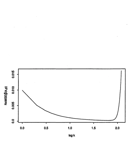
That is, the effect of the initial valuePo persists even in the limit.

In order to illustrate the mildness of the first assumption of Theorem 1, Figure 2 shows the typical shape ofN x M S E(fr, k, p) as a function of k. Figure 3 shows this same function plotted

It)

....

Q:

~

<g, 0

w

....

en

:E

)(

z

It)

o

o

100 200 300

k

400 500 600

,,.

.It)

....

0

d

c:

0

_....

¥. 0

e

d

w UJ

::e

₎₍ It)

Z 0

0

d

o d

0.0

0.5

1.0

Iogk

1.5

2.0

Figure 3: The normaJized mean squared error function N xMSE(y, k,p)for N = 20 and p.= 0.01,

4

Comparing the three methods

Methods 1 and 2 (equations (4) and (5» share the questionable property that the recommended group size remains the same; regardless of the number of tests, N, being performed. Method 3 (equation (6» recommends different group sizes for different valueS ofN.

The criterion on which Method 1 is based, namely equalizing the absolute influence of a group showing the trait and the influence of a group not showing the trait, has some appeal, but seems to be of less practical interest than the criteria behind Methods 2 and 3, namely minimizing the asymptotic variance or the exact mean squared error, respectively. In practice, these are the quantities by which estimators are usually evaluated. Comparing Methods 2 and 3, although the asymptotic variance might be an adequate approximation to the mean squared error when N is large, it may be very misleading when N is small. Overall, based on these arguments alone, one might prefer Method 3 for determining the group size to be used for data collection.

Asymptotically, Methods 2 and 3 are equivalent, since limN_coke(N) = kG' To make an asymptotic comparison of Methods 1 and 2, one needs to compare the values of the asymptotic variance of

p

evaluated when k

=

ki and when k

=

kG' The asymptotic variance of

p

when k

=

ki is 2.0814(1- p)2[ln(1 -

p)]2/N.

The value when k = kG is 1.5441(1- p)2[ln(1-

p)]2/N.

Hence, a procedure using kG to obtain the group size is asymptotically 2.0814/1.5441

=

1.35 times more efficient than one using ki. Moreover, since kG and ke are asymptotically equivalent, a procedure

that uses ke to obtain the group size is also asymptotically 1.35 times more efficient than one using

ki. Therefore, Methods 2 and 3 are preferable to Method 1 in an asymptotic sense.

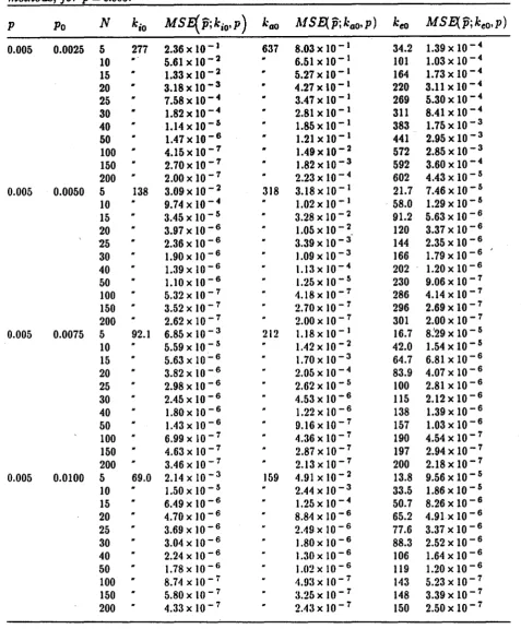
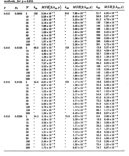
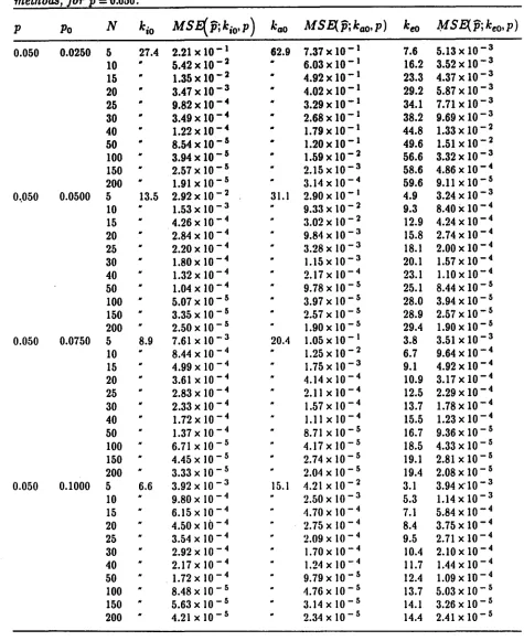
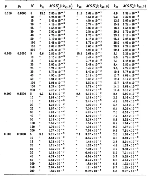
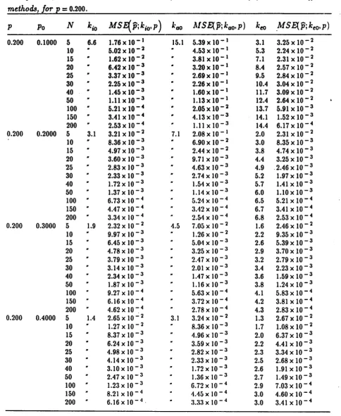
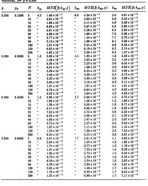
Tables 1-8 present further comparisons of these methods for choosing the group size for several

...

choices of p, Po, and N. For each value of p, the values of Po shown are Po = 0.5p, p, 1.5p, and 2p. The tables show the values ofkiO, kGo and keD for these choices, as well as the true mean squared error of

p

obtained with these different group sizes. For example, considerp

=

0.01. When

.~

to 69, 159 and 65, respectively. The (true) mean squared errors (MSE's) of

p

when N = 20 for these group sizes are 1.29 x 10-5, 1.04X 10-2 and 1.28 x 10-5, respectively. In this example, the

MSE's with kiO and kea are very similar. WhenPo= 0.015= 1.5p, then kiO= 45.9, kao = 105 and

k_ea(20) = 45.7. The (true) mean squared errors of

p

when N = 20, are 1.52 x 10-5, 2.08 X 10-4

and 1.52X10-5• Once again, the MSE's withkiO andk_{ea are very similar. Now suppose}Po= 0.015

andN = 200. Then kiO =45.9, kao= 105 and ken= 99.8. The corresponding mean squared errors are 1.38 x 10-6_{, 8.49X 10-}7 _{and 8.67 x 10-}7_{• In this case,kao and kea give similar MSE's.}

There are several observations that can be made from Tables 1-8. In general, recommended group sizes decrease aspincreases. Also, for fixed N andp, the recommended group size (kiO, kao, orken) decreases asPo increases.

Insupport of Result 1, it is seen that asN gets larger,ken indeed approaches kao (from below). It is also seen that kiO is always exceeded by kao, and that kea starts below kiO for small N,then increases towards kao as N increases.

The dependence ofkiO, kao, and ken on the initial valuePo,can be summarized as three different cases. WhenPo=p,that is, when the initial value equals the truep, thenkea provides the smallest

mean squared error. Indeed, this is no surprise since ken was derived to minimize the mean squared error. However, kiO is a close second for small N and kao is a close second for large N.

Now consider Po

<

p. In this case, all methods choose larger group sizes than they did when Po =p. WhenN is such that kiO

<

k_ea

<

_kao (usually when N is large), the group sizekiO provides the smallest mean squared error, with ken yielding the next smallest, and _kao the largest. HN is such thatk_ea

<

kiO

<

kao (usually when N is small), then ken provides the smallest mean squared "":.. "" "error, with _{kiO giving the next smallest, and again kao the largest.}

Finally, considerPo

>

p. In this case, all methods recommend a smaller group size than they did when Po = p. When N is such that kiO

<

ken

<

k_ao (usually when N is large), the group

obtained with kiO. IfN is such. that keD

<

kiO

<

k40 (usually when N is small), either keD or kiO (usually keD)provides the smallest mean squared error, with the other providing the next smallest, and k40 the largest.

Thus, there are cases wherein each. of the three methods performs best, sometimes much. better

than the other two, in recommending a group size to reduce the mean squared error of

p.

However,

the group size keD of Method 3 consistently gave the smallest or second-smallest mean squared error. It seemingly balances the advantages and disadvantages of the other methods. Of the three

methods considered in this section, we recommend Method 3 overall.

5

An iterative method for choosing the group size through a

multistage procedure

Section 2.2 discussed different methods for obtaining the group size when only one group size is to

be used throughout the experiment. However, in a multistage procedure, one could alter the group

size to be used in the next stage of experimentation according to the data collected as of the end

of the previous stage. For example, at the beginning of an experiment one might have an initial

value, Po, for the proportion, and use that value to obtain a group size by any of the methods of

Section 2.2, or any other method. A number, say Nt, of groups of this size are then tested and an estimate of the proportion,

P

NI , is obtained. It is then decided that data collection will continue,

but that the group size to be used will now be redetermined using

P

NI in place ofPo. The group

size for the second stage is then a function ofPo and of the data collected in the first stage. The

'.:...data for the second stage are then collected and a new estimate

P

Nl+_N2 is obtained, where N₂is

the number of groups in the second stage. One could repeat the process of obtaining a new group

size based on the information accumulated to that point as often as desired. The question arises

addresses that question.

Let N represent the total number of tests to be performed over allstages; AiN is the number of tests performedin the

i'h

stage, where i ~ 1 and Al

+... +

Ai = ~i ~ 1; PiiN is the estimate of the proportion obtained at the end of the ith stage; and k;~+lNis the group size for stage i

+

1,

rAiN

obtained using the estimateP>'iN'for i ~ 0 andPioN

=

Po.

Method 3 of Section 2.2 will be used to determine the group size. That is,

where

and 8h

=

1 - (1 - p)h. Result 2 describes the limiting behavior of these group sizes, when the

intermediate estimatesP>'iN' i ~ 0, are strongly consistent for p.

Result 2 Suppose the estimator P>'iN is such that with probability one, 0

<

P>'iN

<

1 for all

N

>

Ni andPiiN

~1

pasN - 00. Then, provided that with probability one the first derivative of

Q>'i+_1N(k;Pi.N) with respect to k equals zero at most once, and ka,

<

00, andk;~:~N(N) ~ 1for

•

alli ~ 0and N

>

Ni,

where i ~ 0 and ka, is as defined in Section 2.2.2.

The proof is given in the Appendix. [Result 1 is obtained as a special case by lettingi = 0,Al = 1 and Po = p.] Result 2 says that, even if the proportion used to obtain the group size varies with

probability one to the true proportion, as N tends to infinity. Moreover, the limit is independent of the initial value Po. Inother words,ifthe intermediate estimates are strongly consistent, then as the total number of tests increases, the group size for the next stage approaches the optimal group size with probability one, whatever the value ofPo.

6

Discussion and conclusions

Three criteria for determining the size to be used for the groups in the usual group-testing procedure for the estimation of proportions have been presented and compared. Of these three, the one that has the greatest practical appeal is the criterion of minimizing the exact mean squared error of the estimator

p.

Under this method, the group size selected depends on the number of tests to be performed, as well as on the initial value Poone uses in place of the true value of the proportion

p. Moreover, as the number of tests increases, this method converges to that based on minimizlng the asymptotic variance. As a result, when the number of tests is large, one could approximate the group size obtained from the method based on minimizing the mean squared error by using the

r

group size obtained from minimizing the asymptotic variance. The group size obtained by equating the absolute value of the influence of a group showing the trait with one not showing the trait provides an estimate with a smaller mean squared error when the number of tests is small, but is not, in general, the method of choice.

-::. ".

single-group-size procedureslackthe ability to overcome the misinformation provided byPo, since they do not alter the group size throughout the experiment as does the recursive method in a

multistage procedure. As the quality ofPois often unknown in practice, the multistage procedure offers an appealing way to avoid an estimate with potentially large bias and mean squared error,

resulting from a poor choice ofPo. The possible advantages of the multistage procedure will be addressed in detail in a subsequent paper.

References

[1] Chen, C. L. (1987). Estimation problems in group testing. Ph.D. dissertation, North Carolina

State University, Raleigh, N.C.

[2] Chen, C. L. and Swallow, W. H. (1990). Using group testing to estimate a proportion, and to

test the binomial model. Biometrics 46, 1035-1046.

[3] Chiang, C. L. and Reeves, W. C. (1962). Statistical estimation of virus infection rates in

mosquito vector populations. American Joumal of Hygiene 75, 377-391.

[4] Gibbs, A. J. and Gower, J. C. (1960). The use of a multiple-transfer method in plant virus transmission studies-some statistical points arising in the analysis of results. Annals of Applied

Biology48(1),75-83.

[5] Griffiths, D. A. (1972). A further note on the probability of disease transmission. Biometrics

28, 1133-1139.

[6] Kerr, J. D. (1971). The probability of disease transmission. Biometrics 27, 219-222.

[7] Loyer, M. (1983). Bad probability, good statistics, and group testing for binomial estimation.

[8] Peto, S. (1953). A dose response equation for the invasion of micro-organisms. Biometrics 9, 320-335.

[9] Sobel, M. and Elashoff, R. M. (1975). Group testing with a new goal, estimation. Biometrika 62, 181-193.

[10] Swallow, W. H. (1985). Group testing for estimating infection rates and probabilities of disease

transmission. Phytopathology 75, 882-889.

[11] Swallow, W. H. (1987). Relative mean squared error and cost considerations in choosing group

size for group testing to estimate infection rates and probabilities of disease transmission. Phy-topathology77, 1376-1381.

[12] Thompson, K. H. (1962). Estimation of the proportion of vectors in a natural population of

insects. Biometrics18, 568-578.

APPENDIX: PROOF OF RESULT 2

Define the function Q(kjp) =

J(l~;~~'J.

The proof consists of two main parts. First, it will be

shown that

Then it will be shown that

'".:. "...

Proof: Itis convenient to write the function

Q

lIi+1N(kjp>'i_{N )} as a conditional expectation:

where

and

Let i>'iN= !(1 - _{6iiN )} for N ~ 1. Then 0

<

i>'iN

<

1, 6>'iN

+

i>'iN

<

1 for all N ~ 1, and

6>'iN ~1!(1- 6) as N _ 00,where 6=1- (1- p)h. Then

Case 1: YAi+1N ~ _(6iiN

+

i>'iN)Ai+lN

Then

This implies that

Moreover,

So that

is uniformly integrable. But(1-oiiN-iiiN)2

~1

l(1-0)2,I (YAi+lN

<

(OiiN

+

iiiN)Ai+lN)

~

1 and !(YAi+lN)

~

[P(t-6)]

X~.

Hence

Therefore,

Part!: Show that

Proof: Since Q(klliP)

<

Q(kiP)ifk:f: kll, then for all 0

>

0, there exists €

>

0 (€depends on 0)

such that

Q(kll

- OiP) - Q(klliP)

>

€

and

Q(kll

+

_{0iP) - Q(klliP)}

_>

€.

Furthermore, by Part 1 above, with probability one there exists Nesuch that for all N

>

Nt.,

IQ'\;+IN(kll - DiPi;N) - Q(kll- DiP)1

<

i'

IQ'\;+1N(kB

+

iiPi;N) - Q(kB

+

OiP)1

<

i·

which implies

Similarly,

SinceQ>'i+lN(k;p~iN)is continuously differentiable in k,then its derivative with respect tokequals

zero for somek E (kCl

- 6, kCl

+

6),N

>

N_u k:~+1N(N) E (kCl- 6, kCl

+

6) with probability one. That

"iN

is, limN_cok:~+lN(N)E (kCl

- 6,kCl

+

6) with probability one. But 6 is arbitrary, so

Table 1

Group sizes, and their associated mean squared errors, arising from three different methods, for

p

=

0.001.

P Po N k;o MSE{Pik;oIP) kao MS~PikaoIP) keo

!J

sEt

Pikeol

p)

0.001 0.0005 5 1386 2.37 x 10-1 3186 8.08 x 10-1 98.6 1.01 x 10-5 10 5.63 x 10-2 6.55 x 10-1 364 7.43 x 10-6

15 " 1.34x10-2 " 5.31 x 10-1 646 1.48 x 10-5

20 3.17x10-3 _{4.30 x 10-}1 _{905 3.18 x 10-}5

25 7.53x10-4 3.48 x 10-1 1137 6.35 x 10-5

30 1.79 x 10-4 " 2.82 x 10-1 1345 1.17xl0-4

40 1.01X10-5 1.85X10-1 1700 3.14xl0-4

50 6.04X10-7 1.21 x 10-1 1993 6.64 x 10-4

100 1.67X10-8 1.48 x 10-2 2840 2.44 x 10-3

150 1.09 x 10-8 _{1.80 x 10-}3 _{2953 3.26 x 10-}4 200 8.05 x 10-9 _{2.19 x 10 - 4 3015 4.33 x 10-}5

0.001 0.0010 5 693 3.12xl0-2

159:' 3.21 x 10-1 62.4 5.05 x 10-6

10 9.75X10-4 1.03x10-1 209 6.78·x 10-7

15 3.06 x 10-5 3.31 x 10-2 _{358 2.69 x 10-}7

20 1.07 x 10-6 _1.06xl0-2 _{492 1.53 x 10-}7

"25 1.24 x 10-7 3.41 x 10 - 3 610 1.04 x 10-7

30 7.75xl0-8 1.l0xl0-3 _{716 7.71xlO-}8

40 5.59 x 10-8 1.13 x 10-4 _{895 5.04 x 10-}8

50 4.40X10-8 1.17xlO-5 1041 3.73 x 10-8

100 2.14 x 10-8 1.69 x 10-8 1427 1.66 x 10-8 ·150 1.41 x 10-8 1.09 x 10-8 _{1481 1.08x10-}8 200 1.05 x 10-8 8.03 x 10-9 1508 8.02 x 10-9

0.001 0.0015 5 462 6.92 x 10-3 1062 1.20 x 10-1 47.8 5.66 x 10-6

10 4.83 x 10 - 5 1.43 x 10 - 2 ₁₅₁ 8.22 x 10-7

15 5.46 x 10-7 1.72 x 10-3 253 3.33 x 10-7 20 1.56 x 10-7 2.06 x 10-4 344 1.90 x 10-7 25 1.20 x 10-7 2.48 x 10 - 5 424 1.27 x 10-7 30 9.84 x 10-8 3.03 x 10-6 495 9.37 x 10-8

40 7.24xlO-8 8.98 x 10-8 _{615 5.99 x 10-}8

50 5.73 x 10-8 3.74 x 10-8 712 4.34 x 10-8 100 2.81 x 10-8 _{1.75 x 10 - 8 953 1.82 x 10-}8 150 1.86 x 10 -8 1.15xl0-8 987 1.18 x 10-8 200 1.39 x 10- 8 8.57 x 10-9 _{1004 8.74xl0-}9

0.001 0.0020 5 346 2.15x 10-3 796 4.98 x 10 - 2 39.6 6.59xl0-6

10 5.04 x 10-6 _{2,48 x 10-}3 _{120 1.01xlO-}6

15 2.70 x 10 - i 1.24 x 10 - .. 198 4.09x 10-7 20 1.89 x J.O - 7 6.30 x 10-6 267 2.32 x 10-7 25 1.48 x 10-7 3.97 x 10-7 328 1.55 x 10-7 30 1.22 x 10-7 8.71 x 10-8 _{381 1.13 x 10-}7

...

40 9.01 x 10-8 5.22 x 10- 8 471 7.14xl0-8

50 7.14xlO-8 4.IOx 10- 8 543 5.12 x1.0-8

100 3.51xlO- 8 1.98xl0- 8 715 2.10xl0- 8

150 2.32 x 10- 8 1.31 x 10 - 8 740 1.36 x 10-8

Table 2

Group sues, and their associated mean squared errors, arising from three different

methods, for p=0.005.

P Po N

k

io MSE{fi;kiO'p) kao AIS~p; kao'p) keo MS~p;keo,P)

0.005 0.0025 5 277 2.36xI0-1 _{637 8.03 x 10-}1 _{34.2 1.39 x 10-}4

10

..

5.61 x 10-2 6.51xl0-1 _{101 1.03x10-}4

15 1.33 x 10-2 5.27X10-1 164 1.73 x 10-4

20 3.18 x 10-3 _4.27X10-1 _{220 3.11 x 10-}4

25 7.58xI0-4 _{3.47 x 10-}1 _{269 5.30 x 10-}4

30 1.82 x 10-4 2.81xl0-1 _{311 8.41 x 10-}4

40 1.14 x 10-5 _1.85X10-1 _{383 1.75xl0-}3

50 1.47 x 10-6 _1.21X10-1 _{441 2.95 x 10-}3 100 4.15 x 10-7 1.49X10-2 572 2.85 x 10-3 150 2.70 x 10-7 1.82 x 10-3 _{592 3.60 x 10-}4

200 2.00 x 10-7 _{2.23 x 10-}4 _{602 4.43 x 10-}5

0.005 0.0050 5 138 3.09 x 10-2 318 3.18xI0-1 21.7 7.46 x 10 - 5 10 9.74 x 10-4 1.02xl0-1 ·58.0 1.29 x 10 - 5

15 3.45 x 10-5 _3.28xl0-2 _{91.2 5.63 x 10-}6

20 3.97 x 10-6 _{1.05 x 10 - 2_ 120 3.37 x 10-}6

25 2.36 x 10-6 _{3.39 x 10-}3 _{144 2.35 x 10-}6

30 1.90 x 10-6 _{1.09 x 10 - 3 166 1.79 x 10-}6

40 1.39 x 10-6 1.13xlO-4 _{202 1.20 x 10-}6

50 1.10xl0-6 1.25 x 10-5 _{230 9.06 x 10-}7

100 5.32xl0-7 _{4.18x 10-}7 _{286 4.14xl0-}7

150 3.52xl0-7 2.70 x 10-7 296 2.69 x 10-7

200 2.62xl0-7 2.00 x 10-7 301 2.00 x 10-7

0.005 0.0075 5 92.1 6.85 x 10-3 212 1.18xl0-1 _{16.7 8:29 x 10-}5 10 5.59 x 10 - 5 1.42 x 10 - 2 42.0 1.54 x 10 - 5 15 5.63 x 10-6 1.70 x 10 - 3 64.7 6.81 x 10-6 20 3.82 x 10-6 2.05 x 10-4 _{83.9 4.07 x 10-}6

25 2.98 x 10-6 _2.62xl0-5 _{100 2.81 x 10-}6

30 2.45 x 10-6 _4.53xl0-6 _{115 2.12xI0-}6

40 1.80 x 10-6 _{1.22 x 10-}6 _{138 1.39 x 10 - 6}

50 1.43xl0-6 _9.16xlO-7 _{157 1.03 x 10-}6

100 6.99 x 10-7 _{4.36x 10-}7 _{190 4.54 x 10-}7

150 4.63 x 10-7 2.87 x 10-7 197 2.94 x 10-7

200 3.46 x 10-7 2.13X10-7 200 2.18xI0-7

0.005 0.0100 5 69.0 2.14 x 10 -3 159 4.91xl0-2 13.8 9.56 x 10-5 10 1.50 x 10 - 5 2.44 x 10-3 _{33.5 1.86 x 10 - 5}

15 6.49 x 10-6 1.25 x 10-4 _{50.7 8.26 x 10-}6

20 4.70x 10-6 8.84 x 10-6 65.2 4.91xlO-6

25 3.69 x 10-6 2.49x 10-6 77.6 3.37 x 10-6 30 3.04 x 10-6 1.80 x 10 - 6 88.3 2.52xl0-6 40 2.24 x 10-6 1.30 x 10 - 6 106 1.64 x 10-6

50 1.78 x 10 - 6 1.02 x 10 -6 119 1.20 x 10-6

100 8.74xl0-7 4.93X10-7 143 5.23 x 10-7

150 5.80 x 10 - 7 3.25 x 10-7 148 3.39 x 10-7

Table 3

Group sues, and their associated mean squared errors, arising from three different methods, for P=0.010.

P Po N kio MSFi... p;kiOIP) kao MS~p;kaoIP) keo MS~p;keoIP) 0.010 0.0050 5 138 2.34 x 10-1 318 7.95xIO-1 21.7 4.23 x 10-4

10 5.59 x 10-2 _{6.45 x 10-}1 _{58.0 3.07 x 10-}4

15 1.33 x 10-2 5.23 x 10-1 91.2 4.76xI0-4

20 3.19 x 10-3 4.25 x 10-1 120 7.88x·l0-4

25 7.68xl0-4 3.45 x 10-1 144 1.25 x 10-3

30 1.88 x 10-4 2.80 x 10-1 166 1.85 x 10-3 40 1.50 x 10-5 1.84 x 10-1 202 3.42 x 10-3 50 4.14 x 10-6 _{1.21 x 10-}1 _{230 5.21 x 10-}3

100 1.65 x 10-6 _1.50x10-2 _{286 2.89 x 10-}3

150 1.07 x 10-6 1.85 x 10-3 _{296 3.69 x 10-}4

200 7.97xI0-7 2.30 x 10-" 301 4.73xl0-5 0.010 0.0100 5 69.0 3.07 x 10-2 159 3.15xIO-1 _{13.8 2.37 x 10-}4

10 9.85 x 10-4 1.01X10-1 33.5 4.58 x 10 - 5

15 4.69 x 10-5 _{3.25 x 10 - 2 50.7 2.08 x 10 - 5}

20 1.29x 10-5 1.04 x 10 - 2 65.2 1.28 x 10 - 5

25 9.31 x 10-6 3.36 x 10-3 _{77.6 9.01 x 10-}6

30 7.57 x 10-6 1.08 x 10-3 _{88.3 6.92 x 10-}6

40 5.53X10-6 1.16x10-4 106 4.71 x 10-6

50 4.36 x 10-6 1.51x10-5 _{119 3.58xl0-}6

100 2.12 x 10-6 1.66 x 10 - 6 143 1.65 x 10-6 150 1.40 x 10 - 6 1.08x10-6 148 1.07 x 10-6

200 1.04 x 10-6 7.96 x 10-7 150 7.94 x 10-7 0.010 0.0150 5 45.9 6.81 x 10-3 _{105 1.17xlO-}1 _{10.6 2.62 x 10-}4

10 8.07 x 10 - 5 1.39 x 10 - 2 24.3 5.40 x 10-5 15 2.14x10-5 1.67 x 10 -3 35.9 2.49 x 10 - 5

20 1.52 x 10 - 5 2.08 x 10-4 45.7 1.52xl0-5 25 1.19xlO-5 _{3.17 x 10 - 5 54.0 1.07 x 10 - 5}

30 9.74 x 10-6 9.32 x 10-6 _{61.0 8.10xl0-}6

40 7.18 x 10-6 _{4.71 x 10-}6 _{72.5 5.39xl0-}6

50 5.68 x 10-6 _{3.64 x 10-}6 _{81.0 4.01 x 10-}6

100 2.78 x 10-6 _{1.74 x 10-}6 _{94.8 1.80 x 10-}6

150 1.84 x 10 -6 1.14xlO-6 98.1 1.17xl0-6

200 1.38 x 10-6 8,49xl0-7 _{99.8 8.67 x 10-}7

0.010 0.0200 5 34.3 2.16 x 10-3 i8.9 4.82x 10-2 _{8.8 3.00 x 10-}4

10 4.59 x 10 - 5 2.39 x 10-3 19.3 6.49 x 10 - 5

15 2.58 x 10 - 5 1.33 x 10 - 4 28.1 3.00 x 10 - 5

20 1.87 x 10 - 5 l.71x10-5 35.5 1.82 x 10-5

25 1.47 x 10 - 5 9.02 x 10-6 41.7 1.27 x 10 - 5

.'.:. -. 30 1.21 x 10 - 5

7.12xlO-6 _{46.9 9.59 x 10-}6

40 8.94 x 10-6 5.17 x 10-6 _{55.3 6.31 x 10-}6

50 7.09 x 10-6 _{4.06x 10-}6 _{61.5 4.66 x 10-}6

100 3.49 x 10-6 _{1.97 x 10-}6 _{71.0 2.08 x 10-}6

•

Table ..

Group sIZes, and their associated mean squared errors, arising from three different

methods, for

p

=0.020.

P Po N kio MSE{pjkio,p) kao MS!lpjkao,p) keo MS!lpjkeo,p)

0.020 0.0100 5 69.0 2.31 x 10-1 159 7.81x10-1 13.8 1.27 x 10-3

10 5.54x10-2 6.34 x 10-1 33.5 8.98 x 10-4

15 1.33 x 10-2 5.16xl0-1 _{50.7 1.27 x 10-}3

20 3.23 x 10-3 4.19 x 10-1 65.2 1.93 x 10-3

25 7.99 x 10-4 3.41xl0-1 77.6 2.82 x 10-3

30 2.10xl0-4 2.77xl0-1 88.3 3.90 x 10-3

40 2.89 x 10-5 _{1.83 x 10-}1 _{106 6.39 x 10-}3 50 1.47 x 10 - 5 1.21 x 10-1 119 8.68 x 10-3 100 6.52xl0-6 1.52 x 10 - 2 143 3.00 x 10-3 150 4.25 x 10-6 1.92X10-3 148 3.91 x 10-4 200 3.16 x 10-6 2.46 x 10-4 _{150 5.43 x 10-}5

0.020 0.0200 5 34.3 3.02 x 10-2 78.9 3.09 x 10-1 _{8.8 7.43 x 10-}4

10 1.05 x 10-3 9.9IxI0-2 19.3 1.62 x 10-4

15 9.63 x 10-5 3.19 x 10 - 2 28.1 7.69xl0-5 20 4.83 x 10 - 5 1.03 x 10-2 35.5 4.81xlO-5

25 3.67 x 10-5 3.32 x 10-3 41.7 3.45xl0-5

30 2.99 x 10-5 1.08 x 10-3 46.9 2.67 x 10-5 40 2.19 x 10 - 5 1.28x10-4 55.3 1.84 x 10 - 5

50 1.72 x 10-5 2.57 x 10-5 61.5 1.41 x 10-5 100 8.38xl0-6 6.57 x 10-6 71.0 6.52 x 10-6 150 5.54 x 10-6 _{4.26 x 10-}6 _{73.4 4.24 x 10-}6

200 4.13xl0-6 3.15xI0-6 74.7 3.14 x 10-6

0.020 0.0300 5 22.8 6.8IxI0-3 52.3 1.14x10-1 _{6.8 8.15 x 10-}4

10 1.80 x 10 - 4 1.35 x 10-2 14.0 1.89 x 10-4 15 8.34 x 10 - 5 1.65 x 10-3 19.9 9.08 x 10-5 20 6.00 x 10 - 5 2.30 x 10-4 24.8 5.67 x 10-5 25 4.69xI0-5 5,43 x 10 - 5 28.9 4.02 x 10-5 30 3.86 x 10 - 5 2.84 x 10 - 5 32.3 3.09xl0-5 40 2.84 x 10 -5 1.85 x 10 - 5 37.7 2.08 x 10-5

50 2.25xI0-5 1.44 x 10 - 5 41.5 1.57x10-5

100 I.IOxlO-5 6.88 x 10-6 47.1 7.15 x 10-6 150 7.31 x 10 -6 4.52x 10-6 48.7 4.64 x 10-6

200 5.46 x 10-6 3.36 x 10-6 _{49.6 3.43 x 10-}6

0.020 0.0400 5 17.0 2.36x 10-3 39.0 4.65x 10-2 5.6 9.27 x 10-4 10 1.68 x 10 - 4 2.35 x 10-3 ILl 2.25 x 10-4 15 1.02 x 10 - 4 1.72 x 10 - 4 _15.6 1.09 x 10-4

20 7.4IxlO-5 5.02 x 10 - 5 19.2 6.75xl0-5

25 5.83 x 10 -5 3,48 x 10-5 22.2 4.77xl0-5

30 4.80xI0-5 2.8IxlO-5 24.8 3.64 x 10 - 5

."

3.55 x 10 - 5 2.05 x 10 - 5 2.43 x 10 - 5

40 28.7

50 2.82 x 10 - 5 1.61X10-5 31.3 1.82 x 10 - 5

Table 5

Group sizes, and their associated mean squared errors, arising from three different methods, for p

=

0.050.

P Po N

k

io MSE{pj

k

io'p) kao AfSE(pj kao' p)

k

eo MSE(pjkeo,p)

0.050 0.0250 5 27.4 2.21 x 10-1 62.9 7.37xl0-1 _{7.6 5.13 x 10-}3

10 5.42 x 10-2 6.03 x 10-1 16.2 3.52 x 10-3 15 1.35 x 10-2 4.92 x 10-1 23.3 4.37 x 10-3 20 3.47X10-3 4.02X10-1 29.2 5.87 x 10-3

25 9.82 x 10-4 _3.29X10-1 _{34.1 7.71xl0-}3

30 3.49 x 10-4 _{2.68 x 10-}1 _{38.2 9.69 x 10-}3

40 1.22 x 10-4 1.79 x 10-1 44.8 1.33 x 10-2 50 8.54xl0-5 1.20 x 10-1 49.6 1.51 x 10 - 2

100 3.94 x 10-5 _{I.S9x 10-}2 _{56.6 3.32 x 10-}3

150 2.57 x 10-5 2.15 x 10-3 58.6 4.86 x 10-4

200 1.91xl0-5 3.14xl0-4 _{59.6 9.11 x 10-}5

0..050 0.0500 5 13.5 2.92 x 10 - 2 31.1 2.90 x 10-1 4.9 3.24 x 10-3 10 1.53 x 10 - 3 9.33 x 10 - 2 9.3 8.40xl0-4

15 4.26 x 10 -4 3.02 x 10 - 2 12.9 4.24 x 10-4

20 2.84 x 10 - 4 9.84 x 10-3 15.8 2.74xl0-4 25 2.20 x 10-4 3.28 x 10-3 _{18.1 2.00 x 10-}4

30 1.80 x 10 - 4 1.15 x 10-3 20.1 1.57 x 10-4

40 1.32 x 10 - 4 2.17 x 10 - 4 23.1 1.l0xl0-4

• 50 1.04 x 10-4 _{9.78 x 10 - 5 25.1 8.44 x 10 - 5}

100 5.07 x 10 - 5 3.97xl0-5 28.0 3.94 x 10-5

150 3.35 x 10-5 2.57 x 10-5 _{28.9 2.57 x 10-}5

200 2.50 x 10 - 5 1.90xl0-5 29.4 1.90 x 10 - 5

0.050 0.0750 5 8.9 7.61 x 10-3 _{20.4 1.05 x 10-}1 _{3.8 3.51 x 10-}3

10 8.44xl0-4 _{1.25 x 10 - 2 6.7 9.64xl0-}4

15 4.99 x 10-4 _{1.75 x 10-}3 _{9.1 4.92 x 10-}4

20 3.61 X10-4 4.14xl0-4 10.9 3.17xl0-4

25 2.83 x 10-4 2.11 x 10-4 _{12.5 2.29 x 10-}4

30 " 2.33 x 10-4 1.57 x 10-4 _{13.7 1.78xl0-}4

40 1.72 x 10-4 l.11xlO-4 _{15.5 1.23 x 10-}4

50 1.37 x 10 -4 8.71 x 10-5 16.7 9.36 x 10 - 5

100 6.71X10-5 4.17xl0-5 18.5 4.33 x 10-5

150 4.45 x 10 - 5 2.74xl0-5 19.1 2.81 x 10-5

200 3.33 x 10 - 5 2.04 x 10 - 5 19.4 2.08 x 10 - 5

0.050 0.1000 5 6.6 3.92 x 10-3 15.1 4.21 x 10-2 3.1 3.94)(10-3

10 9.80 x 10-4 _{2.50 x 10-}3 _{5.3 1.14xl0-}3

15 6.15xl0-4 _{4.70x 10-}4 _{7.1 5.84 x 10-}4

20 4.50x 10-4 _{2.75 x 10-}4 _{8.4 3.75 x 10-}4

25 3.54 x 10-4 _{2.09 x 10-}4 _{9.5 2.71 x 10-}4

... 30 2.92 x 10 - 4 1.70 x 10 - 4 10.4 2.10 x 10-4

40 2.17 x 10 - 4 1.24 x 10-<1 11.7 1.44 x 10 - 4

50 1.72 x 10 - <I 9.79x 10-5 12.4 1.09 x 10 - 4

100 8.48xl0-5 4.76xlO-5 13.7 5.03 x 10 - 5

Table 6

Group sues, and their associated mean squared error~, arising from three different

methods, for p=0.100.

P Po N kio MSF{p;kiO'p) kao MSElp;kao'p) keo MSElp;keo'p)

0.100 0.0500 5 la·5 2.05 x 10-1 31.1 6.68 x 10-1 _{4.9 1.38 x 10-}2 10 5.26 x 10-2 5.51 x 10-1 9.3 9.32 x 10-3

15 1.41 x 10-2 _4.54xl0-1 _{12.9 1.05 x 10-}2

20 4.18x 10-3 3.74 x 10-1 15.8 1.28 x 10-2

25 1.55 x 10-3 _3.09X10-1 _{18.1 1.54 x 10-}2

30 7.92xl0-4 2.54X10-1 20.1 1.79 x 10-2

40 4.26 x 10-4 1.73 x 10-1 _{23.1 2.12xlO-}2

50 3.19 x 10-4 1.18 x 10-1 25.1 2.05 x 10-2 100 1.48 x 10-4 1.73 x1O~2 28.0 4.01 x 10-3 150 9.69 x 10 - 5 2.66 x 10-3 28.9 7.27xl0-4 200 7.20xl0-5 _{4.96 x 10-}4 _{29.4 2.05 x 10-}4 0.100 0.1000 5 6.6 2.89 x 10 - 2 15.1 2.61 x 10 - 1 3.1 9.21 x 10-3

10 3.15xl0-3 8.44 x 10 - 2 5.3 2.79 x 10-3

15 1.50 x 10 - 3 2.78 x 10 - 2 7.1 1.48 x 10-3

20 1.05xl0-3 9.48 x 10 - 3 8.4 9.83 x 10-4

25 8.21 x 10-4 _{3.49 x 10 -3 9.5, 7.29 x 10-}4 30 6.73X10-4 1.49 x 10 -3 10.4 5.78 x 10-4 40 4.95xl0-4 5.19 x 10 -4 11.7 . 4.09 x 10-4

50 3.91 x 10-4 _{3.36 x 10-}4 _{12.4 3.17xl0-}4

100 1.91xlO-4 _{1.50 x 10-}4 _{13.7 1.48 x 10-}4 150 1.27 x 10-4 _{9.71 X10-}5 _{14.1 9.68 x 10-}5

200 9.46 x 10 - 5 7.19xl0-5 14.4 7.18 x 10-5 0.100 0.1500 5 4.3 l.11xlO-2 _{9.8 9.15xl0-}2 _{2.4 9.90 x 10-}3

10 2.98 x 10-3 _{1.18 x 10-}2 _{3.9 3.16 x 10-}3 15 1.86 x 10-3 _{2.41 x 10 -3 4.9 1.70 x 10-}3 20 1.36 x 10 - 3 1.06 x 10 -3 5.8 1.13xl0-3

25 1.07 x 10 - 3 ;.:10 x 10-·1 _{6.4 8.29xl0-}4

30 8.83 x 10 - 4 5.81X10-.1 _7.0 6.53 x 10-4

40 6.54xl0-4 _4.19xlO-·1 _{7.7 4.57 x 10-}4

50 5.19x 10-4 _{3.28 x 10-}4 _{8.1 3.52 x 10-}4

100 2.56 x 10 - 4 1.58 x 10 -4 8.9 1.64 x 10-4

150 1.70 x 10 - 4 1.04xl0-4 9.2 1.07 x 10-4 200 1.27 x 10 - 4 7.76xl0-5 9.3 7.91 x 10-5 0.100 0.2000 5 3.1 9.21xlO-3 _{7.1 3.67xl0-}2 _{2.0 1.10xl0-}2

10 3.63 x 10-3 3.65xl0-3 3.0 3.69X10-3

15 2.33 x 10-3 1.48 x 10 - 3 _3.8 2.01 x 10-3

20 1.71xlO-3 _{1.02 x 10 - 3 4.4 1.33 x 10-}3

25 1.35 x 10 - 3 7.90xl0-4 4.9 9.80 x 10-4

0 " • 30

1.12xl0-3 _{6.46 x 10 - 4 5.2 7.71xlO-}4

40 8.33 x 10-4 _{4.74x 10-}4 _{5.7 5.38 x 10-}4

50 6.63 x 10-4 _3.74xlO-4 _{6.0 4.14xl0-}4

100 3.28 x 10-4 _{1.82 x 10 -4 6.5 1.93 x 10-}4

150 2.18xl0-4 _1.21xlO-4 _{6.7 1.25 x 10-}4

Table 7

Group sIZes, and their associated mean squared errors, arising from three different

methods, for

p

=

0.200.

P

Po

N kio

MSF{ Pi

kiO'

P)

l~ao

J.!SD.Pi kao'

p) k_eo

.MSD.Pikeo,P)

0.200 0.1000 5 6.6 1.76xl0-1 _{15.1 5.39 x 10 - 1 3.1 3.25 x 10 - 2}

10 5.02 x 10-2 4.53 x 10-1 _{5.3 2.24x10-}2

15 1.62 x 10-2 _{3.81 x 10-}1 _{7.1 2.31 x 10-}2

20 6.42x10-3 3.20 x 10-1 _{8.4 2.57 x 10-}2

25 3.37 x 10-3 2.69X10-1 9.5 2.84x10-2

30 2.25 x 10-3 _{2.26 x 10-}1 _{10.4 3.04 x 10 - 2}

40 1.45 x 10-3 1.60 x 10-1 _{11.7 3.09 x 10-}2

50 1.11 x 10-3 _{1.13 x 10-}1 _{12.4 2.64 x 10-}2

100 5.21 x 10-4 _{2.05 x 10-}2 _{13.7 5.91 x 10-}3

150 3.41xl0-4 _4.13xlO-3 _{14.1 1.52 x 10-}3

200 2.53X10-4 I.lIxlO-3 14.4 6.17x10-4

0.200 0.2000 5 3.1 3.21 x 10-2 _{7.1 2.08 x 10-}1 _{2.0 2.31X10-}2

10 8.36 x 10-3 6.90X10-2 3.0 8.35x 10-3

15 4.97 x 10-3 2.44 x 10-2 _{3.8 4.74x10-}3

20 3.60x 10-3 9.7IxI0-3 4.4 3.25 x 10-3

"25 2.83 x 10-3 4.63 x 10-3 4.9 .2.46x10-3 30 2.33 x 10-3 _{2.74 x 10-}3 _{5.2 1.97 x 10-}3 40 1.72 x 10-3 _{1.54 x 10-}3 _{5.7 1.41 x 10-}3

" 50 1.37 x 10 - 3 1.14X10-3 6.0 I.lOx10-3

100 6.73 x 10-4 5.24 x 10-4 _{6.5 5.21 x 10-}4

150 4.47xI0-4 _{:1.42 x 10-}4 _{6.7 3.41 x 10-}4

200 3.34 x 10-4 _{2.54 x 10-}4 _{6.8 2.53 x 10 - 4}

0.200 0.3000 5 1.9 2.32 x 10 -2 4.5 7.05 x 10-2 _{1.6 2.46 x 10-}2

10 9.97 x 10-3 _{1.26 x 10-}2 _{2.2 9.35 x 10-}3

15 6.45 x 10-3 _{5.04 x 10 - 3 2.6 5.39x10-}3

20 4.78 x 10-3 3.25 x 10-3 _{2.9 3.70x10-}3

25 3.79 x 10-3 2.47 x 10 -3 3.2 2.79 x 10-3

30 3.14xI0-3 _2.01X10-3 _{3.4 2.23 x 10-}3

40 2.34 x 10-3 _1.47x10-3 _{3.6 1.59 x 10-}3

50 1.87 x 10-3 _{1.16 x 10-}3 _{3.8 1.24 x 10-}3

100 9.27x 10-4 _{5.63 x 10-}4 _{4.1 5.83 x 10-}4

150 6.16x 10-4 _{3.72x 10-}4 _{4.2 3.81 x 10-}4

200 4.62x 10-4 _{2.78 x 10-}4 _{4.3 2.83 x 10-}4

0.200 0.4000 5 1.4 2.65 x 10":2 3.1 3.24 x 10 - 2 _1.3 2.67 x 10 - 2

10 1.27 x 10 - 2 8.36 x 10-3 _{1.7 1.08 x 10 - 2}

15 8.37 x 10-3 _{4.96 x 10-}3 _{2.0 6.37 x 10-}3 20 6.24 x 10-3 _{3.59 x 10-}3 _{2.2 4.41 x 10-}3 25 4.98 x 10-3 _{2.82 x 10-}3 _{2.3 3.34 x 10-}3

-::. ". 30 4.14xI0-3 2.33 x 10 -3 2.5 2.68 x 10-3

40 3.IOx 10-3 1.72 x 10 -3 2.6 1.91 x 10 - 3

50 2.47 x 10-3 _1.36xl0-3 _{2.7 1.49 x 10-}3

100 1.23 x 10 -3 6.72x 10-4 _{2.9 7.03 x 10-}4

150 8.21 x 10-4 _{4A5x 10-}4 _{3.0 4.60 x 10-}4

Table 8

Group sues, and their associated mean squared errors, arising from three different methods, for P=0.300.

P Po N kio MSE(PikiO'P) kao MSElPikao,P) keo MSElPikeo,P) 0.300 0.1500 5 4.3 1.48 x 10-1 9.8 4.24 x 10-1 _{2.4 4.81 x 10-}2

10

.

4.81X10-2 3;63 x 10-1 3.9 3.43 x 10-2

15 1.86 x 10-2 3.11xl0-1 4.9 3.39 x 10-2

20 9.09 x 10-3 _{2.67 x 10-}1 _{5.8 3.60 x 10 - 2}

25 5.61 x 10-3 2.29 x 10-1 6.4 3.80 x 10 - 2

30 4.09 x 10-3 1.96xl0-1 7.0 3.90 x 10 - 2

40 2.77xl0-3 1.44 x 10-1 _{7.7 3.70xl0-}2

50 2.13xl0-3 1.06 x 10-1 8.1 3.08xl0-2

100 1.01X10-3 2.41xl0-2 8.9 8.45 x 10-3

150 6.63 x 10-" 6.19xlO-3 _{9.2 2.74xl0-}3 200 4.93 x 10-" 2.08X10-3 9.3 1.27 x 10-3 0.300 0.3000 5 1.9 3.80 x 10 - 2 4.5 1.63x10-1 _{1.6 3.56 x 10-}2

10 1.46x10-2 5.63 x 10-2 _{2.2 1.44 x 10-}2

15 9.26 x 10-3 2.23xl0-2 2.6 8.55 x 10-3

20 6.8Ixl0-3 1.06 x 10 - 2 2.9 6.00 x 10-3

"25 5.39 x 10-3 _{6.24 x 10-}3 _{3.2 4.60 x 10-}3

30 4.46X10-3 4.36 x 10-3 3.4 3.72xl0-3

40 3.32X10-3 2.83X 10-3 3.6 2.69 x 10-3

"

50 2.64 x 10-3 2.16 x 10-3 3.8

2.11xl0-3

100 1.31 x 10 - 3 1.01 x 10 -3 4.1 1.01 x 10-3 150 8.70 x 10-4 _{6.64 x 10-}4 _{4.2 6.62 x 10-}4

200 6.5.2 x 10 - 4 4.94 x 10-4 4.3 4.93 x 10-4

0.300 0.4500 5 1.2 3.88 x 10 - 2 2.7 5.66 x 10-2 1.3 3.75xl0-2

10 1.90x10-2 1.56 x 10 - 2 _1.5 1.60 x 10-2

15 1.26x10-2 _{8.56 x 10-}3 _{1.8 9.71xI0-}3

20 9.41X10-3 6.06 x 10 - 3 1.9 6.85 x 10-3

25 7.52 x 10-3 _{4.73x 10-}3 _{2.0 5.25 x 10-}3

30 6.26 x 10-3 3.89X10-3 2.1 4.25 x 10-3

40 4.69x 10-3 _{2.87 x 10-}3 _{2.3 3.07 x 10-}3

50 3.75 x 10-3 _{2.27 x 10-}3 _{2.3 2.40 x 10-}3 100 1.87 x 10 -3 I.l1xlO-3 2.5 1.15 x 10 - 3 150 1.25 x 10 - 3 7.38 x 10-4 2.5 7.54 x 10-4

200 9.34 x 10-4 _{5.52 x 10-}4 _{2.6 5.61 x 10-}4

0.300 0.6000 5 0.8 5.0IxlO-2 _{1.7 3.61 x 10 - 2 1.1 4.03 x 10-}2 10 2.58 x 10 - 2 1.52 x 10 - 2 1.2 1.85 x 10 - 2

15 1.74 x 10-2 _9.77xlO-3 _{1.3 1.16 x 10-}2

20 1.31 x 10 - 2 7.23xlO-3 1.4 8.30 x 10-3

25 1.05 x 10 - 2 5.74xlO-3 1.4 6.44 x 10-3

30 8.76 x 10-3 4.76xlO-3 1.5 5.25 x 10-3

0 "

40 6.59 x 10 - 3 3.54X 10-3 1.5 3.82 x 10-3 50 5.28 x 10-3 2.82 x 10-3 1.6 3.01 x 10-3 100 2.65 x 10-3 1.40 x 10 - 3 1.7 1.45xl0-3

150 1.76 x 10 - 3 9.33x 10-4 1.7 9.54 x 10-4