Shared Components Topic Models
Matthew R. Gormley Mark Dredze Benjamin Van Durme Jason Eisner
Center for Language and Speech Processing Human Language Technology Center of Excellence
Department of Computer Science Johns Hopkins University, Baltimore, MD
{mrg,mdredze,vandurme,jason}@cs.jhu.edu
Abstract
With a few exceptions, extensions to latent Dirichlet allocation (LDA) have focused on the distribution over topics for each document. Much less attention has been given to the un-derlying structure of the topics themselves. As a result, most topic models generate topics in-dependently from a single underlying distri-bution and require millions of parameters, in the form of multinomial distributions over the vocabulary. In this paper, we introduce the Shared Components Topic Model (SCTM), in which each topic is a normalized product of a smaller number of underlying component dis-tributions. Our model learns these component distributions and the structure of how to com-bine subsets of them into topics. The SCTM can represent topics in a much more compact representation than LDA and achieves better perplexity with fewer parameters.
1 Introduction
Topic models are probabilistic graphical models meant to capture the semantic associations underly-ing corpora. Since the introduction of latent Dirich-let allocation (LDA) (Blei et al., 2003), these mod-els have been extended to account for more complex distributions over topics, such as adding supervision (Blei and McAuliffe, 2007), non-parametric priors (Blei et al., 2004; Teh et al., 2006), topic correla-tions (Li and McCallum, 2006; Mimno et al., 2007; Blei and Lafferty, 2006) and sparsity (Williamson et al., 2010; Eisenstein et al., 2011).
While much research has focused on modeling distributions over topics, less focus has been given to the makeup of the topics themselves. This emphasis
leads us to find two problems with LDA and its vari-ants mentioned above: (1) independently generated topics and (2) overparameterized models.
Independent Topics In the models above, the top-ics are modeled as independent draws from a single underlying distribution, typically a Dirichlet. This violates the topic modeling community’s intuition that these distributions over words are often related. As an example, consider a corpus that supports two related topics, baseball and hockey. These topics likely overlap in their allocation of mass to high probability words (e.g. team, season, game, play-ers), even though the two topics are unlikely to ap-pear in the same documents. When topics are gen-erated independently, the model does not provide a way to capture this sharing between related topics. Many extensions to LDA have addressed a related issue, LDA’s inability to model topic correlation,1 by changing the distributions over topics (Blei and Lafferty, 2006; Li and McCallum, 2006; Mimno et al., 2007; Paisley et al., 2011). Yet, none of these change the underlying structure of the topic’s distri-butions over words.
Overparameterization Topics are most often
parameterized as multinomial distributions over words: increasing the topics means learning new multinomials over large vocabularies, resulting in models consisting of millions of parameters. This issue was partially addressed in SAGE (Eisenstein et al., 2011) by encouraging sparsity in the topics which are parameterized by their difference in log-frequencies from a fixed background distribution. Yet the problem of overparameterization is also tied
1Two correlated topics, e.g.nutritionandexercise, are likely
to co-occur, but their word distributions might not overlap.
to the number of topics, and though SAGE reduces the number of non-zero parameters, it still requires a vocabulary-sized parameter vector for each topic.
We present the Shared Components Topic Model (SCTM), which addresses both of these issues by generating each topic as a normalized product of a smaller number of underlying components. Rather than learning each new topic from scratch, we model a set of underlying component distributions that constrain topic formation. Each topic can then be viewed as a combination of these underlying com-ponents, where in a model such as LDA, we would say that components and topics stand in a one to one relationship. The key advantages of the SCTM are that it can learn and share structure between overlap-ping topics (e.g.baseballandhockey) and that it can represent the same number of topics in a much more compact representation, with far fewer parameters.
Because the topics are products of components, we present a new training algorithm for the sig-nificantly more complex product case which re-lies on a Contrastive Divergence (CD) objective. Since SCTM topics, which are products of distri-butions, could be represented directly by distribu-tions as in LDA, our goal is not necessarily to learn better topics, but to learn models that are substan-tially smaller in size and generalize better to unseen data. Experiments on two corpora show that our model uses fewer underlying multinomials and still achieves lower perplexity than LDA, which suggests that these constraints could lead to better topics.
2 Shared Components Topic Models
The Shared Components Topic Model (SCTM) fol-lows previous topic models in inducing admixture distributions of topics that are used to generate each document. However, here each topic multinomial distribution over words itself results from a normal-ized product of shared components, each a multino-mial over words. Each topic selects a subset of com-ponents. We begin with a review and then introduce the SCTM.
Latent Dirichlet allocation (LDA) (Blei et al., 2003) is a probabilistic topic model which defines a generative process whereby sets of observations are generated from latent topic distributions. In the SCTM, we use the same generative process of topic
assignments as LDA, but replace the K indepen-dently generated topics (multinomials over words) with products ofCcomponents.
Latent Dirichlet allocation generative process
For each topick∈ {1, . . . , K}:
φk∼Dir(β) [draw distribution over words] For each documentm∈ {1, . . . , M}:
θm∼Dir(α) [draw distribution over topics] For each wordn∈ {1, . . . , Nm}:
zmn∼Mult(1,θm) [draw topic]
xmn∼φzmi [draw word]
LDA draws each topic φk independently from a Dirichlet. The model generates each document m
of length M, by first sampling a distribution over topics θm. Then, for each word n, a topic zmn is chosen and a word typexmnis generated from that topic’s distribution over wordsφzmi.
A Product of Experts (PoE) model (Hinton, 1999) is the normalized product of the expert dis-tributions. In the SCTM, each component (an ex-pert) models an underlying multinomial word dis-tribution. We let φc be the parameters of the cth component, whereφcv is the probability of the cth component generating wordv. If the structure of a PoE included only components c ∈ C in the prod-uct, it would have the form: p(x|φ1, . . . ,φC) =
Q c∈Cφcx PV
v=1
Q
c∈Cφcv,where there areC components, and the summation in the denominator is over the vocab-ulary. In a PoE, each component can overrule the others by giving low probability to some word. A PoE can be viewed as a soft intersection of its com-ponents, whereas a mixture is a soft union.
The Beta-Bernoulli model (Griffiths and
Ghahramani, 2006) is a distribution over binary matrices with a fixed number of rows and columns. It is the finite counterpart to the Indian Buffet Process. In this work, we use the Beta-Bernoulli as our prior for an unobserved binary matrixBwithC
the notion that some components area priori more likely to be included in topics.
The Beta-Bernoulli model generative process
For each componentc∈ {1, . . . , C}: [columns] πc∼Beta(Cγ,1) [draw probability of componentc] For each topick∈ {1, . . . , K}: [rows]
bkc∼Bernoulli(πc) [draw whether topic includescth component in its PoE]
2.1 Shared Components Topic Models
The Shared Components Topic Model generates each document just like LDA, the only difference is the topics are not drawn independently from a Dirichlet prior. Instead, topics are soft intersections of underlying components, each of which is a multi-nomial distribution over words. These components are combined via a PoE model, and each topic is constructed according to a length C binary vector
bk; wherebkc = 1includes andbkc = 0excludes componentc. Stacking theKvectors forms aK×C
matrix; rows correspond to topics and columns to components. Overlapping topics share components in common.
Generative process SCTM’s generative process generates topics and words, but must also generate the binary matrix. For each of theC shared com-ponents, we generate a distribution φc over the V
words from a Dirichlet parametrized by β. Next, we generate aK×Cbinary matrix using the Beta-Bernoulli prior. These components and the binary matrix implicitly define the complete set ofKtopic distributions, each of which is a PoE.
p(x|bk,φ) =
QC c=1φbcxkc PV
v=1
QC c=1φ
bkc
cv
(1)
The distribution p(·|bk,φ) defines the kth topic. Conditioned on theseKtopics, the remainder of the generative process, which generates the documents, is just like LDA.
The Shared Components Topic Model generative process
For each componentc∈ {1, . . . , C}:
φc∼Dir(β) [draw distribution over words]
πc∼Beta(Cγ,1) [draw probability of componentc] For each topick∈ {1, . . . , K}:
bkc∼Bernoulli(πc) [draw whether topic includescth component in its PoE]
For each documentm∈ {1, . . . , M}
θm∼Dir(α) [draw distribution over topics] For each wordn∈ {1, . . . , Nm}
zmn∼Mult(1,θm) [draw topic]
xmn∼p(· |bzmn,φ)given by Eq. (1) [draw word]
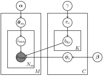
See Figure 1 for the graphical model.
Discussion An advantage of this formulation is the ability to model many topics using few components. While LDA must maintainV×Kparameters for the topic distributions, the SCTM maintains justV ×C
parameters, plus an additionalK×Cbinary matrix. SinceC < K V this results in many fewer pa-rameters for the SCTM.2 Extending the number of topics (rows) requires storing additional binary vec-tors, a lightweight requirement. In theory, we could enable all2C possible component combinations, al-though we expect to use far less. On the other hand, constraining the SCTM’s topics by the components gives less flexible topics as compared to LDA. How-ever, we find empirically that a large number of top-ics can be effectively modeled with a smaller num-ber of components.
Observe that we can reparameterize the SCTM as LDA by assuming an identity square matrix; each component corresponds to a topic in LDA, making LDA a special case of the SCTM with an identity matrix IC. Intuitively, SCTM learning could pro-duce an LDA model where appropriate. Finally, we can also think of the SCTM as learning the struc-ture of many PoE models. In applications where ex-perts abstain, the SCTM could learn in which setting (row) each expert casts a vote.
3 Parameter Estimation
Parameter estimation infers values for model pa-rameters φ, π, and θ from data using an unsuper-vised training procedure. Because exact inference is intractable in the SCTM, we turn to approximate methods. As is common in these models, we will integrate outπandθ, sample latent variablesZand
B, and optimize the componentsφ. Our algorithm follows the outline of the Monte Carlo EM (MCEM) algorithm (Wei and Tanner, 1990). In the Monte Carlo E-step, we will re-sample the latent variables
Z andB based on current model parametersφand observed dataX. In the M-step, we will find new model parametersφ. Since these parameters corre-spond to experts in the PoE, we rely on a contrastive divergence (CD) objective (Hinton, 2002), popular for PoE training, rather than maximizing the data
2The vocabulary sizeV could be much larger if n-grams or
log-likelihood. Normally, CD only estimates the pa-rameters of the expert distributions. However, in our model, the structure of the PoEs themselves change based on the E-step. Since we generate multiple samples in the E-step, we modify the CD objective to compute the gradient for each E-step sample and take the average to approximate the expectation un-derBandZ.3
3.1 E-Step
The E-step approximates an expectation under
p(B, Z|X,φ,α, γ) for latent topic assignments Z
and matrix B using Gibbs sampling. The Gibbs sampler uses the full conditionals for bothzi(7) and
bkc(12), which we derive in Appendix A. Using this sampler, we obtainJ samples ofZ andBby iterat-ing through each value ofzi andbkcJ times (in our experiments, we useJ=1, which appears to work as well on this task as multiple samples). TheseJ sam-ples are then used in the M-step as an approximation of the expectation of the latent variables.
3.2 M-Step
Given many samples ofB andZ, the M-step opti-mizes the component parametersφwhich cannot be collapsed out. We utilize the standard PoE training procedure for experts: contrastive divergence (CD). We approximate the CD gradient as the difference of the data distribution and the one-step reconstruction of the data according to the current parameters. As in Generalized EM (Dempster et al., 1977), a single gradient step in the direction of the contrastive di-vergence objective is sufficient for each M-step. A key difference in our model is that we must incor-porate the expectation of the PoE model structure, which in our case is a random variable instead of a fixed observed structure. We achieve this by simply
3CD training within MCEM is not the only possible
ap-proach. One alternative would be to compute the CD gradient summing over all values ofB and Z, effectively training the entire model using CD. This approach prevents the normal CD objective derivation from being simplified into a more tractable form. Another approach would be a pure MCMC algorithm, which sampledφdirectly. While using the natural parameters allows the sampler to mix, it is too computationally intensive to be practical. Finally, we could train with Generalized MCEM, where the exact gradient of the log-likelihood (or log-posterior) is used, but this easily gets stuck in local minima. After exper-imenting with these and other options, we present our current most effective estimation method.
computing the CD gradient for each PoE given each of the J samples{Z, B}(j) from the E-Step, then
average the result.
Another difficulty arises from computing the gra-dient directly for the multinomialφcdue to theV−1
degrees of freedom imposed by sum-to-one con-straints. Therefore, we switch to the natural pa-rameters, which obviates the need for considering the sum-to-one constraint in the optimization, by defining φc in terms of V real valued parameters {ξc1, . . . , ξcV}:
φcv=
exp(ξcv) PV
t=1exp(ξcv)
(2)
TheV parametersξcvare then used to computeφcv for use in the E-step.
As explained above, the M-step does not maxi-mize the data log-likelihood, but instead minimaxi-mizes contrastive divergence. Hinton (2002) explains that maximizing data log-likelihood is equivalent to min-imizing Q0||Q∞ξ , the KL divergence between the observed data distribution, Q0, and the model’s equilibrium distribution,Q∞ξ .4 MinimizingQ0||Q∞ξ
would require the computation of an intractable ex-pectation under the equilibrium distribution. We avoid this by instead minimizing the contrastive di-vergence objective,
CD(ξ|{Z, B}(j)) =Q0||Q∞ξ −Q1ξ||Q∞ξ , (3)
where Q1ξ is the distribution over one-step recon-structions of the data,XgivenZ, B, ξ, that are gen-erated by a single step of Gibbs sampling.
Unlike standard applications of CD training, the hidden variables (Z,B) are not contained within the experts. Instead they define thestructureof the PoE model, where B indicates which experts to use in each product (topic) andZindicates which PoE gen-erates each word. Unfortunately, CD training cannot infer this structure since the CD derivation makes use of a fixed structure in the one-step reconstruc-tion. Therefore, we have taken a MCEM approach, first sampling the PoE structure in the E-step, then
4
M
Nm
C K
xmn
zmn
θm
α
φc
bkc
πc
γ
[image:5.612.101.278.56.187.2]β
Figure 1: The graphical model for the SCTM.
fixing these samples for Z andB when computing theone-stepreconstruction of the data,X.
Contrastive Divergence Gradient We provide
the approximate derivative of the contrastive di-vergence objective, where Z and B are treated as fixed.5
dCD(ξ|{Z, B}(j))
dξ ≈ −
dlogf(x|bz, φ)
dξ
Q0
+
dlogf(x|bz, φ)
dξ
Q1
ξ
wheref(x|bz, φ) = QCc=1φbcxzc is the numerator of
p(x|bz, φ)and the derivative of its log is efficient to compute:
dlogf(x|bz, φ)
dξcv
=
(
bzc(1−φcv) forx=v −bzcφcv forx6=v
To approximate the expectation underQ1
ξ, we hold
Z, B, ξ fixed and resample the data, X, using one step of Gibbs sampling.
3.3 Summary
Our learning algorithm can be viewed in terms of a Q function: Q(ξ|ξ(t)) ≈
1
J PJ
j=1CD(ξ|{Z, B}(j))where we average over J samples. The E-step computes Q(ξ|ξ(t)). The M-step minimizesQwith respect toξ to obtain the updated ξ(t+1) by performing gradient descent on theQfunction as ξcv(t+1) = ξcv(t)−η· d Q(ξ|ξ
(t))
dξcv for all values ofc, v.
5The derivative is approximate because we drop the term:
−d Q1ξ
dξ · d Q1
ξ||Q ∞ ξ
d Q1
ξ
, which is ‘problematic to compute’ (Hinton,
2002). This is the standard use of CD.
Algorithm 1SCTM Training Initialize parameters:ξc,bkc,zi.
while not convergeddo
{E-step:}
forj= 1toJdo
{Drawjth sample{Z, B}(j)} fori= 1toNdo
Sampleziusing Eq. (7)
fork= 1toKdo forc= 1toCdo
Samplebkcusing ratio in Eq. (12) {M-step:}
forc= 1toCdo forv= 1toV do
Single gradient step overξ
ξ(cvt+1)=ξcv(t)−η·
d Q(φ|φ(t))
dξcv
4 Related Models
The SCTM is closely related to the the Infinite Overlapping Mixture Model (IOMM) (Heller and Ghahramani, 2007), yet our model differs from and, in some ways, extends theirs. The IOMM mod-els the geometric overlap of Gaussian clusters us-ing PoEs, and models the structure of the PoEs with the rows of a binary matrix. The SCTM models a finite number of columns, where the IOMM mod-els an infinite number. The IOMM generates a row for each data point, whereas the SCTM generates a row for each topic. Thus, the SCTM goes beyond the IOMM by allowing the rows to be shared among documents and models document-specific mixtures over the rows of the matrix.6
SAGE for topic modeling (Eisenstein et al., 2011) can be viewed as a restricted form of the SCTM. Consider an SCTM in which the binary matrix is re-stricted such that the first column, b·,1, consists of
all ones and the remainder forms a diagonal matrix. If we then set the first component, φ1, to the cor-pus background distribution, and add a Laplace prior on the natural parameters, ξcv, we have the SAGE model. Note that by removing the restriction that the matrix contain a diagonal, we could allow mul-tiple components to combine in the SCTM fashion, while incorporating SAGE’s sparsity benefits.
6
The relation of TagLDA (Zhu et al., 2006) to the SCTM is similar to that of SAGE and SCTM. TagLDA has a PoE of exactly two experts: one ex-pert for the topic, and one for the supervised word-level tag. Examples of tags are abstract or body, indicating which part of a research paper the word appears in.
Unlike the SCTM and SAGE, most prior exten-sions to LDA have enhanced the distribution over topics for each document. One of the closest is hier-archical LDA(hLDA) (Blei et al., 2004) and its ap-plication to PAM (Mimno et al., 2007). Though top-ics are still generated independently from a Dirich-let prior, hLDA learns a tree structure underlying the topics. Each document samples a single path through the tree and samples words from topics along that path. The SCTM models an orthogonal issue to topic hierarchy: how the topics themselves are represented as the intersection of components. Finally, while prior work has primarily used mix-tures for the sake of conjugacy, we take a fundamen-tally different approach to modeling the structure by using normalized product distributions.
5 Evaluation
We compare the SCTM with LDA in terms of over-all model performance (held-out perplexity) as well as parameter usage (varying numbers of components and topics). We select LDA as our baseline since our model differs only in how it forms topics, which fo-cuses evaluation on the benefit of this model change. We consider two popular data sets for compar-ison: NIPS: A collection of 1,617 NIPS abstracts from 1987 to 19997, with 77,952 tokens and 1,632 types. 20NEWS: 1,000 randomly selected articles from the 20 Newsgroups dataset,8 with 70,011 to-kens and 1,722 types. Both data sets excluded stop words and words occurring in fewer than 10 docu-ments. For20NEWS, we used the standard by-date train/test split. For NIPS, we randomly partitioned the data by document into75%train and25%test.
We compare the SCTM to LDA by evaluating the average perplexity-per-word of the held-out test
7
We follow prior work (Blei et al., 2004; Li and Mc-Callum, 2006; Li et al., 2007) in using only the abstracts: http://www.cs.nyu.edu/˜roweis/data.html
8Williamson et al. (2010) created a similar subset:
http://people.csail.mit.edu/jrennie/20Newsgroups/
data,perplexity=2−log2(data|model)/N. Exact
com-putation is intractable, so we use theleft-to-right al-gorithm(Wallach et al., 2009) as an accurate alter-native. With the topics fixed, the SCTM is equiva-lent to LDA and requires no adaptation of the left-to-right algorithm.
We used a collapsed Gibbs sampler for training LDA and the algorithm described above for training the SCTM. Both were trained for 4000 iterations, sampling topics every 10 iterations after a burn-in of 3000. The hyperparameterα was optimized as an asymmetric Dirichlet, β as a symmetric Dirichlet, andγ= 3.0 was fixed.9Following the observation of Hinton (2002) that CD training benefits from initial-izing the experts to nearly uniform distributions, we initialize the component distributions from a sym-metric Dirichlet with parameterβˆ =1×10⁶. We use
J = 1 samples per iteration and a decaying learning rate centered atη= 100.10We ranged LDA from 10 to 200 topics, and the SCTM from 10 to 100 com-ponents (C). We then selected the number of SCTM topics (K) asK ∈ {C,2C,3C,4C,5C}. For each model, we used five random restarts, selecting the model with the highest training data likelihood.
5.1 Results
Our goal is to demonstrate that (1) modeling topics as products of components is an expressive alterna-tive to generating topics independently and (2) the SCTM can both achieve lower perplexity than LDA and use fewer model parameters in doing so.
Topics as Products of Components Figures 3b
and 3c show the perplexity for the held-out portions of20NEWSandNIPSfor different numbers of com-ponentsC. The shaded region shows the full SCTM perplexity range we observed for different K and at each value of C, we label the number of topics
K (rows in the binary matrix). For each number of components, LDA falls within the upper portion of the shaded region. While for some (small) values of
K for the SCTM, LDA does better, the SCTM can easily include more K (requiring few new param-eters) to achieve better results. This supports our hypothesis that topics can be comprised of the over-lap between shared underlying components.
More-9
On development data the model was rather insensitive toγ.
10
Figure 2: SCTM binary matrix and topics from 3599 training documents of 20NEWSforC = 10,K = 20. Blue squares are “on” (equal to 1).
x
y
5 10 15 202 4 6 8 10
k αk Top words for topic Top words for topic after ablating component c=1 ← 1 0.306 subject organization israel return define law org organization subject israel law peace define israeli ← 2 0.031 encryption chip clipper keys des escrow security law administration president year market money senior ← 3 0.025 turkish armenian armenians war turkey turks armenia years food center year air russian war army ← 4 0.102 drive card disk scsi hard controller mac drives opinions drive hard power support cost research price ← 5 0.071 image jpeg window display code gif color mit pitt file program year center programs image division ← 6 0.018 jews israeli jewish arab peace land war arabs
← 7 0.074 org money back question years thing things point ← 8 0.106 christian bible church question christ christians life ← 9 0.011 administration president year market money senior ← 10 0.055 health medical center research information april ← 11 0.063 gun law state guns control bill rights states ← 12 0.160 world organization system israel state usa cwru reply ← 13 0.042 space nasa gov launch power wire ground air ← 14 0.038 space nasa gov launch power wire ground air ← 15 0.079 team game year play games season players hockey ← 16 0.158 car lines dod bike good uiuc sun cars
← 17 0.136 windows file government key jesus system program ← 18 0.122 article writes center page harvard virginia research ← 19 0.017 max output access digex int entry col line ← 20 0.380 lines people don university posting host nntp time
# of Model Parameters (thousands)
Perple xity 800 1000 1200 1400 ● ● ● ● ● ●● ● ● ● 10 100 11 120 140 2021 40 60 80 10,20 10,30 10,40 10,50 100,200 100,300 100,400 100,500 20,100 20,40 20,60 20,80 40,120 40,160 40,200 40,80 60,120 60,180 60,240 60,300 80,160 80,240 80,320 80,400
0 100 200 300 400 500 600
● LDA
SCTM
(a)
# of Components
Perple xity 800 1000 1200 1400 1600 1800 ● ● ● ●● ● ● ● 10 20 30 40 50 100 200 300 400 500 100 20 40 60 80 120 160 200 40 80 120 180 240 300 60 160 240 320 400 80
0 20 40 60 80 100
● LDA
SCTM
(b)
# of Components
Perple xity 300 400 500 600 700 ● ● ● ●● ● ● ● 10 20 30 40 50 100 200 300 400 500 100 20 40 60 80 120 160 200 40 80 120 180 240 300 60 160 240 320 400 80
0 20 40 60 80 100
● LDA
SCTM
(c)
# of Model Parameters (thousands)
Perple xity 300 350 400 450 500 550 600 ● ● ● ● ● ● ● ● ● ● ● ● ● 10 100 11 120 140 160 180 20 200 21 40 60 80 10,20 10,30 10,40 10,50 100,200100,300 100,400 100,500 20,100 20,40 20,60 20,80 40,120 40,160 40,200 40,80 60,120 60,180 60,240 60,300 80,160 80,240 80,320 80,400
0 100 200 300 400
● LDA
SCTM
(d)
Figure 3: Perplexity results on held-out data for 20NEWS(b) and NIPS (c) showing the results of LDA and the SCTM for the same number of components and varyingK(SCTM). For the same number of components (multinomials), the SCTM achieves lower perplexity by combining them into more topics. Results for 20NEWS(a) and NIPS (d) showing non-square SCTM achieves lower perplexity than LDA with a more compact model.
over, this suggests that our products (PoEs) provide additional and complementary expressivity over just mixtures of topics.
Model Compactness Including an additional
topic in the SCTM only adds Cbinary parameters, for an extra row in the matrix. Whereas in LDA, an additional topic requires V (the size of the vocab-ulary) additional parameters to represent the multi-nomial. In both cases, the number of document-specific parameters must increase as well. Figures 3a and 3d present held-out perplexity vs. number of model parameters on20NEWSandNIPS, exclud-ing the case of square (C =K) binary matrices for the SCTM. The regions show a confidence inter-val (p =0.05) around the smoothed fit to the data,
LDA labels showC, and SCTM labels showC, K. The SCTM achieves lower perplexity with fewer model parameters, even when the increase in non-component parameters is taken into account. We pect that because of its smaller size the SCTM ex-hibits lower sample complexity, allowing for better generalization to unseen data.
5.2 Analysis
k=12αk=0.13 problem state control reinforcement problems models time based decision markov systems function
k=11αk=0.08 learning networks system recognition time network describes hand context views classification
k=14αk=0.07 models images image problem structure analysis mixture clustering approach show computational
k=13αk=0.05 networks network learning distributed system weight vectors property binary point optimal real
k=16αk=0.11 training units paper hidden number output problem rule set order unit show present method weights task
k=15αk=0.12 cells neurons visual cortex motion response processing spatial cell properties patterns spike
k=18αk=0.07 information analysis component rules signal independent representations noise basis
k=17αk=0.10 number functions weights function layer generalization error results loss linear size
k=20αk=0.02 time network weights activation delay current chaotic connected discrete connections
k=19αk=0.03 system networks set neurons visual phase feature processing features output associative c=1 model information parameters kalman robust matrices likelihood experimentally c=2 network networks data learning optimal linear vector independent binary natural algorithms pca c=4 paper units output layer networks patterns unit pattern set rule network rules weights training c=9 visual image images cells cortex scene support spatial feature vision cues stimulus statistics
k=10αk=0.09 neural neurons analog synaptic neuron networks memory time capacity model associative noise dynamics
k=9αk=0.02 vector feature classification support vectors kernel regression weight inputs dimensionality
k=2αk=0.13 network input information time recurrent back propagation units architecture forward layer
k=1αk=0.11 model learning system information parameters networks robust kalman rules estimation
k=4αk=0.12 bayesian results show estimation method based parameters likelihood methods models
k=3αk=0.06 object recognition system objects information visual matching problem based classification
k=6αk=0.23 neural network paper recognition speech systems based results performance artificial
k=5αk=0.04 object recognition system objects information visual matching problem based classification
k=8αk=0.23 algorithm training error function method performance input classification classifier
[image:8.612.80.537.59.326.2]k=7αk=0.08 data paper networks network output feature features patterns set train introduced unit functions
Figure 4: Hasse diagram on NIPS forC = 10,K = 20showing the top words for topics and unrepresented com-ponents (in shaded box). Notice that some topics only consist of a single component. The shaded box contains the components that didn’t appear as a topic. For the sake of clarity, we only show arrows for the subsumption rela-tionships between the topics, and we omit the implicit arrows between the components in the shaded box and the topics.
to the high-level of component re-use across topics. Topics are typically interpreted by looking at the top-N words, whereas the top-N words of a compo-nent often do not even appear in the topics to which it contributes. Instead, we find that the components contribution to a topic is typically through vetoing words. For example, the top words of component
c=1, corresponding to the first column of the binary matrix in figure 2, are[subject organization posting apple mit screen write window video port], yet only a few of these ap-pear in topics k=1,2,3,4,5, which use it.
On the right of figure 2, we show what the top-ics become when we ablate component c=1 from the matrix by setting the column to all zeros. Topic
k=2 changes from being aboutinformation security
togeneral politicsand is identical tok=9. Topick=3 changes fromthe Turkish-Armenian Warto a more generalwar topic. Topic k=4 changes to a less fo-cused version of itself. In this way, we can gain fur-ther insight into the contribution of this component, and the way in which components tend to increase the specificity of a topic to which they are added.
The SCTM sometimes learns identical topics (two rows with the same binary entries “on”) such as
k=13 andk=14 in figure 2 andk=3 andk=5 in fig-ure 4, which is likely due to the Gibbs sampler for the binary matrix getting stuck in a local optimum.
6 Discussion
We have presented the Shared Components Topic Model (SCTM), in which topics are products of underlying component distributions. This model change learns shared topic structures—as expressed through components—as opposed to generating each topic independently. Reducing the number of components yields more compact models with lower perplexity than LDA. The two main limitations of the current SCTM are, when restricted to a square binary matrix (C = K), the inference procedure is unable to recover a model with perplexity as low as a collapsed Gibbs sampler for LDA, and the compo-nents are not consistently interpretable.
The use of components opens up interesting di-rections of research. For example, task specific side information can be expressed as priors or constraints over the components, or by adding conditioning variables tied to the components. Additionally, tasks beyond document modeling may benefit from repre-senting topics as products of distributions. For ex-ample, in vision, where topics are classes of objects, the components could be features of those objects. For selectional preference, components could cor-respond to semantic features that intersect to define semantic classes (Gormley et al., 2011). We hope new opportunities will arise as this work explores a new research area for topic models.
Appendix A: Derivation of Full Conditionals
The model’s complete data likelihood over all variables—observed words X, latent topic assign-mentsZ, matrixB, and component/expert distribu-tionsφ:
p(X, Z, B,φ|α,β, γ) =
p(X|Z, B,φ)p(Z|α)p(B|γ)p(φ|β) (4)
This follows from the conditional independence as-sumptions. It is tractable to integrate out all parame-ters exceptZ, B,φand hyperparametersα,β, γ.11
11For simplicity, we switch from indexing examples asx
mn toxi. In this presentation,xiis theith example in the corpus,
Full conditional of zi Recall that p(Z|α) is the Dirichlet-Multinomial distribution over topic assignments, where θ has been integrated out. The form of this distribution is identical to the corresponding distribution over topics in LDA. The derivation of the full conditional of zi ∈ {1, . . . , K}, follows from the factorization in Eq. 4:
p(zi|X, Z−(i),B,φ,α,β, γ) (5)
∝p(X|Z, B,φ)p(Z|α) (6)
∝p(xi|bzi,φ)(˜n −(i)
mzi +αzi) (7)
Z−(i) is the set of all topic assignments exceptzi. We use the independence of each document, recall-ing that exampleibelongs to documentm. In prac-tice, we cachep(x|bz,φ)for allx, z(V×Kvalues) and these are shared by allziin a sampling iteration. Above, just as in LDA, p(Z|α) is simplified by proportionality to(˜nmz−(ii)+αzi), wheren˜
−(i)
mk is the count of examples for documentmthat are assigned topickexcludingzi’s contribution (Heinrich, 2008).
Full conditional ofbkc Recall thatp(B|γ) is the prior for a Beta-Bernoulli matrix. The full condi-tional distribution of a position in the binary vector is (Griffiths and Ghahramani, 2006):
p(bkc= 1|B−(kc), γ) =
¯
n−c(k)+Cγ
K+Cγ (8)
wheren¯−c(k) is the count of topics with component
cexcluding topick, andB−(kc)is the entire matrix except for the entrybkc.
To find the full conditional forbkc ∈ {0,1}, we again start with the factorization from Eq. 4.
p(bkc|X, Z, B−(kc),φ,α,β, γ) (9)
∝p(X|Z, B,φ)p(B|γ) (10)
∝ "
Y
i:zi=k
p(xi|bzi,φ)
#
p(bkc|B−(kc), γ) (11)
wherep(bkc|B−(kc), γ)is given by Eq. 8,
=
QV
v=1φ ˆ
nkv
cv
bkc
PV
v=1
QC
j=1φ
bkj
jv
−||nˆk||1
p(bkc|B
−(kc), γ)
(12)
and wherenˆkv is the count of words assigned topic
kthat are typev, and||nˆk||1(theL1-norm of count
vectornˆk) is the count ofallwords with topick.
References
David Blei and John Lafferty. 2006. Correlated topic models. InAdvances in Neural Information Process-ing Systems (NIPS), volume 18.
David Blei and Jon McAuliffe. 2007. Supervised topic models. InAdvances in Neural Information Process-ing Systems (NIPS).
David Blei, Andrew Ng, and Michael Jordan. 2003. La-tent dirichlet allocation. Journal of Machine Learning Research, 3.
David Blei, Thomas Griffiths, Michael Jordan, and Joshua Tenenbaum. 2004. Hierarchical topic models and the nested chinese restaurant process. InAdvances in Neural Information Processing Systems (NIPS), vol-ume 16.
A. P. Dempster, N. M. Laird, and D. B. Rubin. 1977. Maximum likelihood from incomplete data via the EM algorithm. Journal of the Royal Statistical Society. Se-ries B (Methodological), 39(1):1–38.
Jacob Eisenstein, Amr Ahmed, and Eric P. Xing. 2011. Sparse additive generative models of text. In Interna-tional Conference on Machine Learning (ICML). Matthew R. Gormley, Mark Dredze, Benjamin Van
Durme, and Jason Eisner. 2011. Shared components topic models with application to selectional prefer-ence. InLearning Semantics Workshop at NIPS 2011, December.
Thomas Griffiths and Zoubin Ghahramani. 2006. Infinite latent feature models and the indian buffet process. In
Advances in Neural Information Processing Systems (NIPS), volume 18.
Gregor Heinrich. 2008. Parameter estimation for text analysis. Technical report, Fraunhofer IGD.
Katherine A. Heller and Zoubin Ghahramani. 2007. A nonparametric bayesian approach to modeling over-lapping clusters. In Artificial Intelligence and Statis-tics (AISTATS), pages 187–194.
Geoffrey Hinton. 1999. Products of experts. In In-ternational Conference on Artificial Neural Networks (ICANN).
Geoffrey Hinton. 2002. Training products of experts by minimizing contrastive divergence. Neural Computa-tion, 14(8):1771–1800.
Wei Li and Andrew McCallum. 2006. Pachinko alloca-tion: DAG-structured mixture models of topic correla-tions. InInternational Conference on Machine Learn-ing (ICML), pages 577–584.
Wei Li, David Blei, and Andrew McCallum. 2007. Non-parametric bayes pachinko allocation. InUncertainty in Artificial Intelligence (UAI).
David Mimno, Wei Li, and Andrew McCallum. 2007. Mixtures of hierarchical topics with pachinko alloca-tion. InInternational Conference on Machine Learn-ing (ICML), pages 633–640.
John Paisley, Chong Wang, and David Blei. 2011. The discrete infinite logistic normal distribution for Mixed-Membership modeling. In International Conference on Artificial Intelligence and Statistics (AISTATS). Yee Whye Teh, Michael Jordan, Matthew Beal, and
David Blei. 2006. Hierarchical dirichlet pro-cesses. Journal of the American Statistical Associa-tion, 101(476):1566–1581.
Hanna Wallach, Ian Murray, Ruslan Salakhutdinov, and David Mimno. 2009. Evaluation methods for topic models. In International Conference on Machine Learning (ICML), pages 1105–1112.
Greg Wei and Martin Tanner. 1990. A monte carlo im-plementation of the EM algorithm and the poor man’s data augmentation algorithms. Journal of the Ameri-can Statistical Association, 85(411):699–704. Sinead Williamson, Chong Wang, Katherine Heller, and
David Blei. 2010. The IBP compound dirichlet process and its application to focused topic model-ing. InInternational Conference on Machine Learn-ing (ICML).