Robust Background Subtraction with Foreground
Validation for Urban Traffic Video
Sen-Ching S. Cheung
Center for Applied Scientific Computing, Lawrence Livermore National Laboratory, 7000 East Avenue, Livermore, CA 94550, USA
Department of Electrical and Computer Engineering, University of Kentucky, Lexington, KY 40506-0503, USA Email:[email protected]
Chandrika Kamath
Center for Applied Scientific Computing, Lawrence Livermore National Laboratory, 7000 East Avenue, Livermore, CA 94550, USA
Email:[email protected]
Received 15 January 2004; Revised 29 December 2004
Identifying moving objects in a video sequence is a fundamental and critical task in many computer-vision applications. Back-ground subtraction techniques are commonly used to separate foreBack-ground moving objects from the backBack-ground. Most
back-ground subtraction techniques assume a single rate of adaptation, which is inadequate for complex scenes such as a traffic
inter-section where objects are moving at different and varying speeds. In this paper, we propose a foreground validation algorithm that
first builds a foreground mask using a slow-adapting Kalman filter, and then validates individual foreground pixels by a simple
moving object model built using both the foreground and background statistics as well as the frame difference. Ground-truth
ex-periments with urban traffic sequences show that our proposed algorithm significantly improves upon results using only Kalman
filter or frame-differencing, and outperforms other techniques based on mixture of Gaussians, median filter, and approximated
median filter.
Keywords and phrases:background subtraction, foreground validation, urban traffic video.
1. INTRODUCTION
Identifying moving objects in a video sequence is a
funda-mental and critical task in video surveillance, traffic
moni-toring and analysis, human detection and tracking, and ges-ture recognition in human-machine interface. A common approach to identifying the moving objects is background subtraction, where each video frame is compared against a reference or background model. Pixels in the current frame that deviate significantly from the background are consid-ered to be moving objects. These “foreground” pixels are further processed for object localization and tracking. Since background subtraction is often the first step in many com-puter vision applications, it is important that the extracted foreground pixels accurately correspond to the moving ob-jects of interest. Requirements of a good background sub-traction algorithm include fast adaptation to changes in
envi-ronment, robustness in detecting objects moving at different
speeds, and low implementation complexity.
At the heart of any background subtraction algorithm is the construction of a statistical model that describes the
background state of each pixel. Different algorithms build the
background model differently, ranging from a single-state
es-timate based on median filter [1,2,3,4,5], Weiner filter [6], or Kalman filter [7,8,9,10,11,12], to a full density estima-tion based on Gaussian mixture models [13,14,15,16,17,
18] or histograms [19]. All of these algorithms have a fixed
design parameter, typically the size of a frame buffer or a re-cursive update parameter, that determines how adaptive the model is to the change in pixel value. We argue that a fixed
parameter is inadequate for scenes such as a traffic
intersec-tion where objects move at a variety of speeds. We illustrate this with an example.
The top plot inFigure 1ashows an example of how a pixel
changes its value throughout a period of time. It begins at level 50, then moves to and stays at 150 for a long period of time. A fast-adapting background subtraction algorithm may output its background/foreground decision similar to the middle plot inFigure 1a: it declares the pixel to be fore-ground for a short period of time before absorbing the new value as part of the background state. On the other hand, the output decision from a slow-adapting algorithm, shown in
the bottom plot inFigure 1a, stays in foreground for a much
Background Foreground
Slow-adapting algorithm
Time Fast-adapting algorithm
Time Background
Foreground
Time t0 t1 t2
50 150
Pix
el
int
ensit
y
(a)
Trail
Slow-adapting algorithm Fast-adapting algorithm
Missing
Trail Space
t2
t1
t0
Ti
m
e
(b)
Ghost
Slow-adapting algorithm Fast-adapting algorithm
Space
t2
t1
t0
Ti
m
e
(c)
Figure1: The top plot in (a) shows the changes of a pixel over time. The middle and bottom plots in (a) show the foreground/background decisions of a fast-adapting and a slow-adapting background subtraction algorithm, respectively. (b) and (c) show two possible scenarios
that may correspond to the plots in (a) at time-stept0,t1, andt2. The top illustration in (b) shows an object moving to the right. The top
illustration in (c) shows another object that is stationary att0but starts to move to the right afterwards, revealing the background behind. The
middle illustrations show the foreground masks produced by a fast-adapting algorithm for the two scenarios at the same time-steps, and the bottom illustrations show those of a slow-adapting algorithm. The dotted arrows indicate where the pixel values and foreground/background decisions in (a) are sampled at the three time-steps.
The issue here is that depending on the particular situa-tion, either of these algorithms can be wrong. One scenario
is shown in the top illustration inFigure 1b, where an object
of gray value 150 is moving slowly to the right over a back-ground of gray value 50. The resulting foreback-ground masks of a fast-adapting and a slow-adapting algorithms are shown in the middle and bottom illustrations. The slow-adapting al-gorithm clearly produces better results as the fast-adapting algorithm misses most parts of the moving object. The prob-lem of a fast-adapting algorithm failing to detect the motion of a homogeneous object is known as the aperture
prob-lem in computer vision [20]. Notice that both algorithms
leave a trail of erroneous foreground pixels behind the ob-ject as their background models are temporarily corrupted
by it. Another possible scenario is shown inFigure 1c, where
an object of gray value 50, stationary at first, starts moving and reveals a background of value 150. The fast-adapting algorithm quickly absorbs the newly revealed background value and correctly identifies the moving object. The slow-adapting algorithm, however, leaves a ghost impression of the object long after it is gone. These two scenarios demonstrate that a single fixed rate of adaptation is not sufficient for
ob-jects moving at different and varying speeds.
The above example also illustrates that it is impossible to determine the correct rate of adaptation by just consider-ing the causal history of a sconsider-ingle pixel. In this paper, we pro-pose a novel algorithm that first builds a foreground mask based on a slow-adapting algorithm, and then validates in-dividual foreground pixels by a simple moving object model
built using both the foreground and background statistics as well as a fast-adapting algorithm. Our primary focus is on
detecting moving vehicles and pedestrians in urban traffic
video taken during day time. This would help us to track the objects in the video, enabling us to build models of nor-mal activity at a scene, and detect anonor-malous events. These models could include the number of vehicles, the paths fol-lowed by the vehicles, their speed, and so forth. This paper is organized as follows: we describe the proposed algorithm in Section 2and contrast it with related work inSection 3. We apply our proposed algorithm and other background
subtraction techniques on a set of urban traffic video
se-quences. Results of subjective evaluations and objective per-formance measurements with respect to a ground-truth are
presented inSection 4. InSection 5, we conclude the paper
by discussing limitations of our algorithm and possible fu-ture work.
2. PROPOSED ALGORITHM
This section describes our proposed algorithm for validat-ing a foreground mask computed by a slow-adaptvalidat-ing
back-ground subtraction algorithm.Figure 2shows the schematic
diagram of our algorithm. The output is a binary foreground
mask Ft at timetwithFt(p) = 1 indicating a foreground
pixel detected at locationp. There are three inputs to the al-gorithm: (1)Itis the video frame at timet; (2)Ptis the binary foreground mask from a slow-adapting background
z−1: \: U:
Delay Set difference Union Video frame
It Slow-adapting
mask,Pt
Frame difference mask,Dt
Object histogram creation Background histogram
creation
Object extension z−1
Core object identification
Blob formation
U Ft \
E0t, Et1, . . . O0
t, O1t, . . . B0t, B1t, . . .
Figure2: Structure of the data validation module.
by thresholding on the normal statistics of the difference
be-tweenItandIt−1, that is,Dt(p)=1 if It(p)−It−1(p)−µd
σd > Td
, (1)
and zero otherwise.µdandσdare the mean and the standard
deviation ofIt(q)−It−1(q) for all spatial locationsq.
Frame-differencing is the ultimate fast-adapting background
sub-traction algorithm. Even though it suffers from severe
aper-ture problem, we choose frame-differencing because it leaves
only a short foreground trail behind a moving object as its memory does not extend beyond the previous frame. There are five key components in our algorithm: blob formation, core object identification, background histogram creation, object histogram creation, and object extension. Their func-tions are explained in the following secfunc-tions.
2.1. Blob formation
In blob formation, all the foreground pixels inPtare grouped
into disconnected blobsBt0,B1t,. . .,BNt based on the assump-tion that each foreground pixel is connected to all of its eight
adjacent foreground pixels [20]. A blob may contain (1) no
object, (2) part of a moving object, (3) a single moving ob-ject with possible foreground trail, and (4) multiple moving objects. The first case corresponds to the foreground ghost
as explained inSection 1. The second case is likely the
re-sult of the aperture problem. SincePtis computed by a
slow-adapting algorithm, the aperture problem occurs only when an object is starting to move. Most blobs fall into the third case of a single object. The last case of multiple objects
oc-cur when multiple vehicles start moving after a traffic light
has turned green. We ignore the last case as the large blob is likely to break down into multiple single-object blobs once
the traffic disperses. The main goals of our algorithm are (1)
to eliminate all the ghost blobs, (2) to maintain the partial-object blobs so that they can grow to contain the full partial-objects,
and (3) to produce better localization for single-object blobs by removing any foreground trail. We accomplish these goals
by validating each blob with the frame-difference maskDtin
the core object identification module.
2.2. Core object identification
The core object identification module first eliminates all the
blobs that do not contain any foreground pixels from Dt.
This step removes all the ghost blobs which produce no
sig-nificant frame differences as there are no moving objects in
them. The module then computes a core objectOit for each
of the remaining blobsBti.Otiis defined as follows:
Oi
t=bounding ellipse
p:p∈Bi
t,Dt(p)=1
∩Bi
t. (2)
We illustrate our definition ofOtiusing a single moving
ob-ject as shown inFigure 3a. The blob contains both the
ob-ject and its foreground trail. The frame-difference maskDt
captures the front part of the object and the small area trail-ing the object, but completely ignores the rest of the fore-ground trail of the blob. Taking advantage of the shape of a typical vehicle, we assume that the object is contained within
the bounding ellipse of all the foreground pixels fromDt
in-side the blob. The key idea is that we can use the bound-ing ellipse to exclude most of the foreground trail from the blob. The bounding ellipse is computed by first calculating its two foci and orientation based on the first- and
second-order moments of the foreground pixels inDt[21], and then
increasing the length of its major axis until it contains all the foreground pixels. Finally, we output the intersection
be-tween the bounding ellipse and the blob shown inFigure 3b
as the core objectOti.
2.3. Background histogram creation
Our experience with urban traffic sequences indicates that
+ +
Object movement
Frame-difference maskDt BlobBi
t Moving object
Bounding ellipse
(a)
+
Object movement
Core objectOit Moving object
(b)
+
Occlusion
Object movement
Frame-difference maskDt BlobBti
Moving object
Bounding ellipse
(c)
Object movement
Boundary ofOit−1 Moving object
at timet-1
Boundary ofOi t
(d)
Figure3: (a) The bounding ellipse is defined by the frame-difference foreground pixels within the blob; (b) the intersection of the bounding ellipse and the blob identifies the core objectOi
t; (c) the bounding ellipse may fail to include the full object emerging from occlusion; (d) the
intersection of the core objects at timet−1 andtis used for estimating the object histogram.
corresponding core objects. Nevertheless, there are situations where the core object captures only a small portion of the en-tire moving object. Consider the example of a vehicle
emerg-ing from an occlusion as shown inFigure 3c. Even though the
blob may contain the entire moving object, the foreground
pixels from Dt are present only in the front, resulting in a
small core objectOitcovering that part of the object. The
ob-ject extension module inFigure 2is responsible for thrusting
back some of the blob pixels outsideOi
tback into foreground.
For every pixelpinBi
toutsideOit, the object extension mod-ule declarespto be foreground ifpis more likely to be part of
the core objectOtithan part of the background. This process
is explained in more detail inSection 2.4. The module thus
needs to estimate the probability density functions (PDF) of both the background and the object.
To estimate the background PDF, we first
parti-tion the current video frame into M rectangular regions
R1,R2,. . .,RM. Then, for each regionRj, we compute a back-ground histogramhtjfor all the pixels inRjthat are not part ofPt, that is,
htj(s)=
p:p∈Rj, P
t(p)=0,It(p)=s p:p∈Rj,P
t(p)=0
(3)
for j =1, 2,. . .,M. In our implementation, we partitionIt
intoM=64 identical rectangular regions.
2.4. Object histogram creation and object extension
To build the object histogram, we notice fromFigure 3bthat
the core objectOti, as defined in (2), may contain pixels that
are not part of the object. It is shown in [6] that the only
pixels guaranteed to be part of the object are pixels fromIt−1
that are foreground in both Dt andDt−1. Based on our
ex-perience, this approach does not always produce sufficient
number of pixels to reliably estimate the object histogram. Instead, for each core objectOit, we first identify the
corre-sponding core object at timet−1, which we denote asOi
t−1.
We accomplish this by finding the core object at timet−1
that has the biggest overlap withOi
t. Then, we compute the
intersection betweenOitandOit−1and build the histogram of
the pixels fromIt−1under this intersection. This procedure
is illustrated inFigure 3d. The object histogramgtifor core objectOi
tcan now be defined as follows:
gti(s)=
p:p∈Oi
t∩Oit−1,It−1(p)=s
p:p∈Oi
t∩Oit−1
Combining the histograms from (3) and (4), the object
ex-tension module defines the object exex-tensionEi
tas those pix-els withinBitbut outsideOitthat are more likely to be part of the core object than of the background:
Eti=
p:p∈Bit\Oit,gti
It(p)
≥htj
It(p)
withp∈Rj. (5)
The final output maskFtis simply the union of all the core
objectsOitand the object extensionsEti.
3. RELATED WORK
In this section, we review related work in background mod-eling and foreground validation. We first summarize some of the representative schemes for background modeling. A
more detailed exposition can be found in [22]. We classify
background modeling algorithms into nonrecursive and re-cursive techniques. A nonrere-cursive technique maintains a
buffer of video frames and uses a sliding-window approach
for background estimation. In order to keep a long history with low storage requirement, video frames can be stored
into the buffer at a frame rater lower than the input rate.
The most commonly used nonrecursive technique is median filtering [1,2,3,4,5]. The background estimate is defined to be the median at each pixel location of all the frames in the buffer. Wiener filter is used in [6], where the filter coef-ficients are estimated at each frame time based on the sam-ple covariances. Unlike median filter or Wiener filter which
produce a single background estimate, Elgammal et al. [19]
build a background PDF using a Gaussian kernel estimator. The advantage of using a full density function over a single estimate is the ability to handle multi modal background dis-tribution. Examples of multi modal background include pix-els from moving leaves of a tree or pixpix-els near high-contrast edges which flicker under small camera movement.
Recursive techniques recursively update a single
back-ground model and do not store a buffer of video frames. The
two simplest recursive techniques are approximated median filter [23,24] and Kalman filter [7,8,9,10,11,12]. Approx-imated median filter increments a running estimate of the median by one if the input pixel is larger than the estimate, and decrements by one if the opposite is true. Kalman filter is a widely used recursive technique for tracking linear
dy-namical systems under Gaussian noise. Many different
ver-sions have been proposed for background modeling, diff
er-ing mainly in the state spaces they use for tracker-ing. We
pro-vide a brief description of the popular scheme used in [7]:
the internal state at pixel locationpof the Kalman filter is
described by the background intensitySt(p) and its temporal derivativeSt(p), which are recursively updated as follows:
St(p) St(p)
=A·
St−1(p) St−1(p)
+K·
It(p)−H·A·
St−1(p) St−1(p)
.
(6)
MatrixAdescribes the background dynamics andHis the
measurement matrix. The Kalman gain matrix K switches
between a slow adaptation rateα1and a fast adaptation rate
α2> α1based on the feedback of the foreground maskFt−1:
K=
α1 α1
ifFt−1(p)=1,
α2 α2
otherwise. (7)
Another popular recursive technique is the mixture of Gaus-sian (MoG), which tracks the background distribution as a
linear sum of K Gaussian component densities [13,14,15,
16,17,18]. If the new input pixelIt(p) is close to one of the Gaussian components, the mean and the standard deviation of that component is updated. Otherwise, the least probable one is deleted and a new component is added, centered at It(p) [14]. The weights of all the components are decayed at
a rate of (1−α), except for the weight of the updated
compo-nent which is incremented byα. To determine which
com-ponents correspond to the background, all comcom-ponents are first ranked by the ratios between their weights and standard
deviations. Then, the firstNcomponents that satisfy the
fol-lowing criterion are declared to be the background compo-nents:
iN
k=i1
ωk,t≥Γ, (8)
whereωk,i1,. . .,ωk,iM are the weights of the components
af-ter ranking, andΓ>0 is the weight threshold.Itis declared
as background if it is withinDtimes the standard deviation
from the mean of any one of the background components. It should be noted that any one of the above-mentioned background modeling algorithms can be used to generate the slow-adapting mask in our proposed algorithm. As described in Section 4, we use Kalman filter in our system primarily because of its simplicity.
Many foreground validation techniques have also been proposed in the literature. Some of them incorporate knowl-edge from the high-level applications such as tracking [9,25],
or use extra information such as depth [25,26] to improve
the background model. Optical flow is also commonly used to detect ghost blobs [5,27]. In contrast to these approaches, our algorithm does not rely on any external information
and uses the much simpler frame-differencing for ghost-blob
removal. Algorithms have also been proposed to combine
multiple background models running at different adaptation
rates [12,19]. However, the combination is done by a
sim-ple conjunction at the pixel level, rather than at the blob level as in our algorithm. Pixel-level combination might lead to the aperture problem as the fast-adapting algorithm can fail to detect slow-moving objects. Blob-level processing has
been proposed in [6] for foreground validation. Similar to
our algorithm, [6] builds core objects based on the
inter-section of a slow-adapting mask and the frame-difference
mask, and grows the core objects using object histograms and connected component grouping. Nevertheless,
lacklus-ter results are reported in [6] because, by growing the core
objects from a waving tree, the blob-level processing turns
part of the sky into foreground. There are three key diff
Table1: Background modeling schemes and their parameters.
Schemes Fixed parameters Test parameter
Frame-differencing (FD) None Foreground thresholdTd
Approximated median filter (AMF) None Foreground thresholdT
Kalman filter (KF) α1=0.001,α2=0.05 Foreground thresholdTk
Median filter (MF) Buffer sizeL=9 Foreground thresholdT
Buffer sampling rater=10 frame/s
Number of componentsK=3
Adaptation rateα=0.05
Mixture of Gaussian (MoG) Weight thresholdΓ=0.25 Deviation thresholdD
Initial varianceσ2 o =36
Initial weightωo=0.1
[6]. First, in our proposed algorithm, the object growing is
confined within the slow-adapting mask, thus limiting the amount of false-positives the algorithm can introduce. Sec-ond, we use both the object histogram and the background histogram to achieve reliable object growing. Finally, using a bounding ellipse as a first-order approximation to the object leads to a significant speedup as it already accounts for most of the foreground pixels.
To summarize, the main advantages of our validation al-gorithm over others in the literature are
(1) our algorithm has low complexity as it does not rely on information from other sensory sources or from so-phisticated computer-vision algorithms. It also mini-mizes the complex blob processing steps by making as-sumptions about the general shape of the foreground objects,
(2) our algorithm achieves good object localization by uti-lizing both foreground and background statistics in combining the slow-adapting blobs with the
frame-difference foreground masks.
4. EXPERIMENTAL RESULTS
In this section, we compare the performance of our proposed algorithm with other algorithms in the literature. We ap-ply the background subtraction algorithms to luminance se-quences only. For preprocessing, we first apply a three-frame
temporal erosion to the test sequence, that is, we replaceIt
with the minimum ofIt−1,It, andIt+1. This step can reduce
temporal camera noise and mitigate the effect of snowfall
present in one of our test sequences. Such an erosion step
is also effective in removing rainfall because raindrops tend
to be much brighter than the surrounding background [28].
On the other hand, this step does not affect the performance
of moving object extraction under normal weather condition because typical object movements are much slower and last much longer than the short transient distortion introduced
by the erosion. Afterwards, a 3×3 spatial Gaussian filter is
used to reduce spatial camera noise.
Even though our proposed algorithm can work with any slow-adapting background subtraction algorithm, we have
chosen Kalman filter as described in Section 3for its
sim-plicity in implementation. To propagate the validation
re-sults to future frames, we use the output maskFt from the
foreground validation for feedback in the Kalman filter. The parameters of the Kalman filter are set as follows [7]:
A=
1 0.7 0 0.7
, H=1 0,
α1=0.001, α2=0.05.
(9)
Similar to the frame-difference thresholding in (1),Pt(p)=1 if
It(p)−St(p)−µk
σk > Tk, (10)
whereSt(p) is the internal state of the Kalman filter, andµk
andσk are the mean and the standard deviation ofIt(q)−
St(q) for all spatial locationsqin the frame. In our
experi-ments, we set the frame-difference foreground thresholdTd
to be 2, and vary the Kalman filter foreground thresholdTkto
show the trade-offbetween false-positives and false-negatives
in foreground detection.
The set of algorithms used for comparison includes
frame-differencing (FD), approximated median filter
(AMF), Kalman filter without validation (KF), median filter (MF), and mixture of Gaussian (MoG). Based on our earlier
work in [22], we have selected particular values for the
parameters in these algorithms that perform well in our test
sequences. These fixed parameters are listed inTable 1. The
most sensitive parameter in each algorithm is used as the test
parameter to show the trade-offbetween false-positives and
false-negatives.
4.1. Test sequences
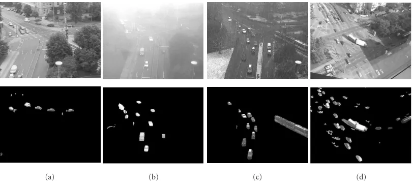
We have selected four publicly available urban traffic video
sequences from the website maintained by KOGS/IAKS,
Uni-versitaet Karlsruhe.1A sample frame from each sequence is
shown in the first row ofFigure 4. The first sequence is called
1The URL ishttp://i21www.ira.uka.de/image sequences. All sequences
(a) (b) (c) (d)
Figure4: Sample frames and the corresponding ground-truth frames from the four test sequences: (a) Bright, (b) Fog, (c) Snow, and (d) Busy.
“Bright,” which is 1500 frames long showing a traffic
in-tersection in bright daylight. The second sequence is called
“Fog,” which is 300 frames long showing the same traffic
in-tersection in heavy fog. The third sequence “Snow” is also 300 frames long and shows the intersection while snowing. Fog and Snow were originally in color; we have first con-verted them into luminance and discarded the chroma chan-nels. The first three sequences all have low to moderate
traf-fic, and contain “stop-and-go” traffic—vehicles come to a
stop in front of a red light and start moving once the light turns green. The last sequence “Busy” is 300 frames long. It shows a busy intersection with the majority of the vehicle traffic flowing from the top left corner to the right side. 4.2. Evaluation
In order to have a quantitative evaluation of the performance, we have selected ten frames at regular intervals from each test
sequence, and manually highlighted all the moving objects in them. These “ground-truth” frames are selected from the lat-ter part of each of the test sequences2to minimize the effect of the initial adaptation of the algorithms. This sampling rate allows the vehicles to move a reasonable distance, making
each ground-truth frame sufficiently different from others.
In the manual annotation, we highlight only the pixels be-longing to vehicles and pedestrians that are actually moving at that frame. Since we do not use any shadow suppression scheme in our comparison, we also include the shadow pix-els cast by moving objects. The ground-truth frames show-ing only the movshow-ing objects are shown in the second row of
Figure 4.
We use two information retrieval measurements, recall and precision, to quantify how well each algorithm matches the ground-truth [29]. They are defined in our context as fol-lows:
Recall=Number of foreground pixels correctly identified by the algorithm
Number of foreground pixels in ground-truth ,
Precision=Number of foreground pixels correctly identified by the algorithm
Number of foreground pixels detected by the algorithm .
(11)
Recall and precision values are both within the range of 0 and 1. When applied to the entire sequence, the recall and precision reported are averages over all the measured frames.
Typically, there is a trade-offbetween recall and precision—
recall usually increases with the number of foreground pixels detected, which in turn may lead to a decrease in precision. A good background algorithm should attain as high a recall value as possible without sacrificing precision.
By varying the testing parameter of each algorithm, we obtain the precision-recall (PR) curves for the test sequences
as shown in Figures5a,5b,5c, and5d. Notice that the PR
curves of all the nonrecursive techniques (FD, AMF, MF)
2The ground-truth frames are selected from the last 1000 frames in the
MF AMF FD
Proposed KF MoG
0 0.2 0.4 0.6 0.8 1
Recall 0
0.1 0.2 0.3 0.4 0.5 0.6 0.7 0.8 0.9 1
P
recision
(a)
MF AMF FD
Proposed KF MoG
0 0.2 0.4 0.6 0.8 1
Recall 0
0.1 0.2 0.3 0.4 0.5 0.6 0.7 0.8 0.9 1
P
recision
(b)
MF AMF FD
Proposed KF MoG
0 0.2 0.4 0.6 0.8 1
Recall 0
0.1 0.2 0.3 0.4 0.5 0.6 0.7 0.8 0.9 1
P
recision
(c)
MF AMF FD
Proposed KF MoG
0 0.2 0.4 0.6 0.8 1
Recall 0
0.1 0.2 0.3 0.4 0.5 0.6 0.7 0.8 0.9 1
P
recision
(d) Figure5: Precision-recall plots for (a) Bright, (b) Fog, (c) Snow, and (d) Busy.
are almost continuous over the entire range of recall values, while those from the recursive ones (MoG, KF, proposed) are discrete, occupying shorter ranges of recall. The reason is that nonrecursive techniques do not have a feedback loop so that it is possible to run the simulation once and compute the pre-cision and the recall for any test parameter value. Recursive
techniques require a separate simulation for each different
test parameter value, and thus we only obtain results at a few operating points.
Figure 5ashows the results of the sequence Bright. The worst performer is FD and the best performer, at least for
re-call above 60%, is our proposed algorithm. Our proposed al-gorithm shares a similar shape with KF but has a much better precision. MoG outperforms the proposed algorithm at low recall primarily because MoG can adapt its threshold for each pixel individually, while our proposed algorithm relies on the global standard deviation. As some of the ground-truth frames have only a few moving objects, the global standard deviation becomes quite small. This turns some of the back-ground pixels into foreback-ground erroneously and thus lowers
the precision values. The PR curves of Fog inFigure 5b
(a) (b) (c)
(d) (e) (f)
Figure6: Foreground images identified by various algorithms showing a moving car and a pedestrian in sequence Bright. (a) FD, (b) AMF, (c) KF, (d) MF, (e)MoG, and (f) proposed.
(a) (b) (c) (d) (e) (f)
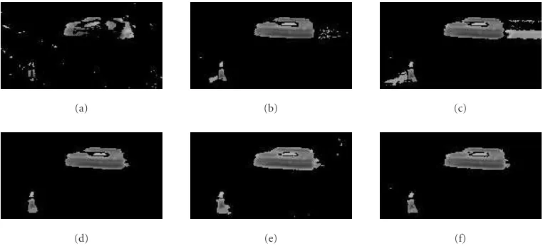
Figure7: Foreground images identified by various algorithms showing a car that starts to move after being stationary for awhile in sequence Snow. (a) FD, (b) AMF, (c) KF, (d) MF, (e)MoG, and (f) proposed.
Figure 5c shows that our proposed algorithm signifi-cantly outperforms all the other schemes in the sequence
Snow. This can be explained by the two thresholds Td and
Tk used in our proposed algorithm. The Snow sequence is
very noisy and all other algorithms need high foreground thresholds to prevent excessive false foreground, thus result-ing in low recall values. On the other hand, our proposed
algorithm can use a small thresholdTkin the Kalman filter
to get good coverage of the moving objects, but uses a large
frame-difference thresholdTdfor building the correct shapes
of the objects and removing the ghost foreground blobs. In the final sequence Busy, our proposed algorithm per-forms worse than MoG and MF for recall values above 60%. This reversal of performance is due to the large number of moving objects clustered together in Busy. At high recall val-ues, the foreground threshold of the Kalman filter is small, creating a large blob that contains many moving objects. The resulting bounding ellipse is not able to eliminate any of the false foreground between vehicles, leading to a low precision value.
We further illustrate the differences between the
al-gorithms using two sets of extracted foreground images
in Figures 6 and 7. The corresponding original images
are shown in Figure 8. Figure 6 is extracted from Bright
showing a car moving to the left and a pedestrian walk-ing to the right. FD is noisy and captures only fragments of the car due to the aperture problem. Both AMF and KF leave a foreground trail behind each moving object as their background states are corrupted. MF, MoG, and
the proposed algorithm produce similar results. Figure 7
(a) (b)
Figure8: (a) and (b) show the original images corresponding to the foreground masks in Figures6and7.
5. CONCLUSIONS
In this paper, we have introduced a new algorithm to validate foreground regions or blobs captured by a slow-adapting background subtraction algorithm. By comparing the blobs
with bounding ellipses formed by frame-difference
fore-ground pixels, the algorithm can eliminate false forefore-ground trails and ghost blobs that do not contain any moving object. Better object localization under occlusion is accomplished by extending the ellipses using the object and background pixel
distributions. Ground-truth experiments with urban traffic
sequences have shown that our proposed algorithm produces performances that are comparable or better than other back-ground subtraction techniques.
Our proposed algorithm, however, has a number of lim-itations. First, the use of bounding ellipses may not be ap-propriate for complex-shaped objects such as human beings.
Second, we use frame-differencing as it produces minimal
false foreground trails behind objects. This assumption may not hold if the input video frame rate is very low. Third, our algorithm relies on the object and background pixel distribu-tions to determine the shape of the foreground objects. If the distributions are not estimated correctly due to lack of sam-ples, or the objects and the foreground have similar pixel dis-tributions, the results will be adversely affected. This problem may be mitigated by extending the time window to incorpo-rate more data as well as using features other than pure pixel intensities. Fourth, inSection 4, we have tested a large range of threshold values and identified the appropriate operating points for our algorithm. In a real system, the thresholds must be automatically adjusted based on the environment. We are currently investigating techniques to adjust thresh-olds automatically by validating the output with an a priori statistical model of foreground objects. Finally, as described inSection 4.2, the proposed algorithm does not perform well when there are multiple moving objects close to each other. We are currently improving our algorithm by building mul-tiple ellipses to identify moving objects and using the back-ground distribution to identify the backback-ground area among them. We will include additional sequences taken under dif-ferent conditions, as well as additional ground-truth frames,
to test how well these enhancements perform in real traffic
sequences.
ACKNOWLEDGMENTS
We would like to thank the two anonymous reviewers for their valuable comments which helped us tremendously in improving the manuscript. UCRL-JRNL-201916: this work was performed under the auspices of the U S Department of Energy by the University of California Lawrence Livermore National Laboratory under Contract no. W-7405-Eng-48.
REFERENCES
[1] B. Gloyer, H. Aghajan, K.-Y. Siu, and T. Kailath, “Video-based freeway monitoring system using recursive vehicle tracking,” inImage and Video Processing III, vol. 2421 ofProceedings of
SPIE, pp. 173–180, San Jose, Calif, USA, February 1995.
[2] R. Cutler and L. Davis, “View-based detection and analysis
of periodic motion,” inProc. 14th International Conference on
Pattern Recognition (ICPR ’98), vol. 1, pp. 495–500, Brisbane, Australia, August 1998.
[3] B. Lo and S. Velastin, “Automatic congestion detection system
for underground platforms,” inProc. International Symposium
on Intelligent Multimedia, Video, and Speech Processing, pp. 158–161, Kowloon Shangri-La, Hong Kong, May 2001. [4] Q. Zhou and J. Aggarwal, “Tracking and classifying moving
objects from videos,” in Proc. 2nd IEEE Workshop on
Per-formance Evaluation of Tracking and Surveillance (PETS ’01), Kauai, Hawaii, USA, December 2001.
[5] R. Cucchiara, C. Grana, M. Piccardi, and A. Prati, “Detecting
moving objects, ghosts, and shadows in video streams,”IEEE
Trans. Pattern Anal. Machine Intell., vol. 25, no. 10, pp. 1337– 1342, 2003.
[6] K. Toyama, J. Krumm, B. Brumitt, and B. Meyers, “Wallflower: principles and practice of background
mainte-nance,” inProc. 7th IEEE International Conference on
Com-puter Vision (ICCV ’99), vol. 1, pp. 255–261, Kerkyra, Greece, September 1999.
[7] K.-P. Karmann and A. Brandt, “Moving object recognition
us-ing and adaptive background memory,” inTime-Varying
[8] D. Koller, J. Weber, and J. Malik, “Robust multiple car track-ing with occlusion reasontrack-ing,” Tech. Rep. UCB/CSD-93-780, EECS Department, University of California, Berkeley, Calif, USA, October 1993.
[9] C. Wren, A. Azarbayejani, T. Darrell, and A. Pentland,
“Pfinder: real-time tracking of the human body,”IEEE Trans.
Pattern Anal. Machine Intell., vol. 19, no. 7, pp. 780–785, 1997. [10] J. Heikkila and O. Silven, “A real-time system for monitoring
of cyclists and pedestrians,” inProc. 2nd IEEE Workshop on
Vi-sual Surveillance (VS ’99), pp. 74–81, Fort Collins, Colo, USA, June 1999.
[11] G. Halevy and D. Weinshall, “Motion of disturbances:
detec-tion and tracking of multi-body non-rigid modetec-tion,”Machine
Vision and Applications, vol. 11, no. 3, pp. 122–137, 1999. [12] T. Boult, R. Micheals, X. Gao, et al., “Frame-rate
omnidirec-tional surveillance and tracking of camuflaged and occluded
targets,” inProc. 2nd IEEE Workshop on Visual Surveillance
(VS ’99), pp. 48–55, Fort Collins, Colo, USA, June 1999. [13] N. Friedman and S. Russell, “Image segmentation in video
se-quences: a probabilistic approach,” inProc. 13th Annual
Con-ference on Uncertainty in Artificial Intelligence (UAI ’97), pp. 175–181, Morgan Kaufmann Publishers, San Francisco, Calif, USA, August 1997.
[14] C. Stauffer and W. Grimson, “Learning patterns of activity
us-ing real-time trackus-ing,”IEEE Trans. Pattern Anal. Machine
In-tell., vol. 22, no. 8, pp. 747–757, 2000.
[15] X. Gao, T. Boult, F. Coetzee, and V. Ramesh, “Error analysis of
background adaption,” inProc. IEEE Conference on Computer
Vision and Pattern Recognition (CVPR ’00), vol. 1, pp. 503– 510, Hilton Head Island, SC, USA, June 2000.
[16] P. KaewTraKulPong and R. Bowden, “An improved adap-tive background mixture model for real-time tracking
with shadow detection,” in Proc. 2nd European Workshop
on Advanced Video-Based Surveillance Systems (AVBS ’01), Kingston, UK, September 2001.
[17] P. W. Power and J. A. Schoonees, “Understanding background
mixture models for foreground segmentation,” inProc. Image
and Vision Computing New Zealand, pp. 267–271, Auckland, New Zealand, November 2002.
[18] D.-S. Lee, J. Hull, and B. Erol, “A Bayesian framework for
Gaussian mixture background modeling,” inProc. IEEE
In-ternational Confererence on Image Processing (ICIP ’03), vol. 3, pp. 973–976, Barcelona, Spain, September 2003.
[19] A. Elgammal, D. Harwood, and L. Davis, “Non-parametric
model for background subtraction,” inProc. IEEE ICCV ’99
Frame-rate workshop, Corfu, Greece, September 1999.
[20] D. H. Ballard and C. M. Brown,Computer Vision,
Prentice-Hall, Englewood Cliffs, NJ, USA, 1982.
[21] R. Mukundan and K. R. Ramakrishnam,Moment Functions in
Image Analysis, World Scientific, Singapore, Singapore, 1998. [22] S.-C. Cheung and C. Kamath, “Robust techniques for
back-ground subtraction in urban traffic video,” in Proc. Video
Communications and Image Processing, SPIE Electronic Imag-ing, San Jose, Calif, USA, January 2004.
[23] N. McFarlane and C. Schofield, “Segmentation and tracking
of piglets in images,”Machine Vision and Applications, vol. 8,
no. 3, pp. 187–193, 1995.
[24] P. Remagnino, A. Baumberg, T. Grove, et al., “An integrated
traffic and pedestrian model-based vision system,” inProc. 8th
British Machine Vision Conference, pp. 380–389, Essex, UK, September 1997.
[25] M. Harville, “A framework for high-level feedback to adap-tive, per-pixel, mixture-of-Gaussian background models,” in
Proc. 7th European Conference on Computer Vision (ECCV ’02), Part III, pp. 543–560, Copenhagen, Denmark, May 2002.
[26] Y. Ivanov, A. Bobick, and J. Liu, “Fast lighting
indepen-dent background,”International Journal of Computer Vision,
vol. 37, no. 2, pp. 199–207, 2000.
[27] D. Gutchess, M. Trajkovic, E. Cohen-Solal, D. Lyons, and A. K. Jain, “A background model initialization algorithm for video
surveillance,” in Proc. 8th IEEE International Conference on
Computer Vision (ICCV ’01), vol. 1, pp. 733–740, Vancouver, British Columbia, Canada, July 2001.
[28] K. Garg and S. Nayar, “Detection and removal of rain from
video,” inProc. IEEE Computer Vision and Pattern Recognition
(CVPR ’04), vol. 1, pp. 528–535, Washington, DC, USA, June 2004.
[29] C. J. van Rijsbergen,Information Retrieval, Butterworth,
Lon-don, UK, 2nd edition, 1979.
Sen-Ching S. Cheungis an Assistant Pro-fessor at the Department of Electrical and Computer Engineering, University of Ken-tucky. He also holds a joint appointment at the Center of Visualization and Virtual Environments, where he and his research group are working on various signal pro-cessing, machine learning, and data min-ing problems in large-scale multimedia sys-tems. Before joining the University of
Ken-tucky, he spent almost two years at Lawrence Livermore National Laboratory working with other data miners on finding abnormal patterns in simulation and surveillance data. He received his Ph.D. degree 2002 from the University of California, Berkeley, based on his work on video summarization, indexing, and clustering. Be-tween 1995 and 1998, he was a Researcher at Compression Labs Inc., San Jose, California, where he developed algorithms for tele-conferencing and satellite broadcast systems. During the same pe-riod, he was also an active participant in the ITU-T H.263 (version 2) and MPEG-4 standardization activities.
Chandrika Kamathis a Computer Scientist at the Center for Applied Scientific Com-puting, Lawrence Livermore National Lab-oratory (LLNL), where she leads the Sap-phire project in scientific data mining. Her research interests include image processing, pattern recognition, and practical applica-tions of data mining. She received her Ph.D. degree in computer science from the Uni-versity of Illinois at Urbana-Champaign in