Volume 2008, Article ID 467928,14pages doi:10.1155/2008/467928
Research Article
Object Delineation by
κ
-Connected Components
Paulo A. V. Miranda, Alexandre X. Falc ˜ao, Anderson Rocha, and Felipe P. G. Bergo
Institute of Computing, University of Campinas, 13084-851 Campinas, SP, Brazil
Correspondence should be addressed to Alexandre X. Falc˜ao,[email protected]
Received 30 November 2007; Revised 27 March 2008; Accepted 2 June 2008
Recommended by Chein-I Chang
The notion of “strength of connectedness” between pixels has been successfully used in image segmentation. We present extensions to these works, which can considerably improve the efficiency of object delineation tasks. A set of pixels is said to be aκ-connected component with respect to a seed pixel, when the strength of connectedness of any pixel in that set with respect to the seed is higher than or equal to a threshold. We discuss two approaches that define objects based onκ-connected components with respect to a given seed set: with and without competition among seeds. While the previous approaches either assume no competition with a single threshold for all seeds or eliminate the threshold for seed competition, we show that seeds with different thresholds can improve segmentation in both paradigms. We also propose automatic and user-friendly interactive methods to determining the thresholds. The proposed methods are presented in the framework of the image foresting transform, which naturally leads to efficient and correct graph algorithms. The improvements are demonstrated through several segmentation experiments involving medical images.
Copyright © 2008 Paulo A. V. Miranda et al. This is an open access article distributed under the Creative Commons Attribution License, which permits unrestricted use, distribution, and reproduction in any medium, provided the original work is properly cited.
1. INTRODUCTION
Image segmentation has been a challenge which involves objectrecognitionanddelineation. Recognition is represented by cognitive tasks that determine the approximate location of a desired object in a given image (object detection), verify the correctness of a segmentation result, and identify a desired object among candidate ones (object classification). Delineation is the task that completes segmentation by defining the precise spatial extent of the desired object in the image. Effective recognition requires object properties while accurate delineation usually depends on image properties to distinguish object and background.
In the context of interactive segmentation, a human operator performs the recognition tasks and the computer performs delineation. In order to make these approaches automatic, we must substitute the human operator by a mathematical model. Model-based approaches have used object properties to build numerical, geometrical, and statistical models for segmentation [1–3], and for simple object detection [4]. Since that a mathematical model usually acts worse than a human expert in the recognition task, it is important to develop interactive methods which minimize
the user’s time and involvement in the delineation process, such that their automation becomes feasible. For example, we are interested in reducing the user intervention to simple selection of a few pixels in the image.
Delineation methods are usually based on a functional of the arc-weights such as graph-cut approaches [5–9] or based on a connectivity functional in the form of a path-cost function [10–13]. This work advances the state-of-the-art of delineation methods based on connectivity functional, being the recognition tasks performed by human operators.
Fuzzy connectedness/watersheds are image segmenta-tion approaches based on seed pixels, which have been successfully used in many applications [10, 14–18]. The relation betweenrelative-fuzzy connectedness[11,19,20] and
image is interpreted as a graph, whose nodes are the image pixels and whose arcs are defined by anadjacency relation
between pixels. The cost of a path in this graph is determined by an application-specificpath-cost function, which usually depends on local image properties along the path—such as color, gradient, and pixel position. For suitable path-cost functions and a set of seed pixels, one can obtain an image partition as an optimum-path forest rooted at the seed set. That is, each seed is root of aminimum-cost path treewhose pixels are reached from that seed by a path of minimum cost, as compared to the cost of any other path starting in the seed set. The IFT essentially reduces image operators to a simple local processing of attributes of the forest [24–28].
The strength of connectedness of a pixel with respect to a seed is inversely related to the cost of the optimum path connecting the seed to that pixel in the graph. In absolute-fuzzy connectedness, the object can be obtained by selecting pixels reached from an internal seed by an optimum path whose cost is less than or equal to a number κ. In this case, the object is said to be a single κ-connected component(a minimum-cost path tree). The object can also be defined as the union of all κ-connected components created from each seed separately, which requires one IFT for each seed. In relative-fuzzy connectedness, seeds selected inside and outside the object compete among themselves, partitioning the image into an optimum-path forest, and the object is defined by the union of the optimum-path trees rooted at its internal seeds. The initial appeal for relative-fuzzy connectedness was the possibility to delineate multiple objects simultaneously, without depending on thresholds. However, the use of thresholding together with seed competition provides a hybrid approach which turns out to be more efficient than the previous ones in many situations. While the previous approaches either assume no competition with a single value of κ for all seeds or eliminateκ for seed competition, we show that seeds with different values ofκcan considerably improve segmentation in both paradigms. Of course, this comes with the problem of finding the values of κ for each seed, but we provide automatic and user-friendly interactive ways to determine them.
Section 2describes some definitions related to the IFT, making them more specific for region-based image seg-mentation. For the sake of simplicity, we will describe the methods for gray-scale and two-dimensional images, but they are extensive to multiparametric and multidimensional data sets. The proposed variants and their algorithms are presented in Sections 3 and4. Section 5demonstrates the improvements with respect to the previous approaches. Conclusion and future work are presented inSection 6.
whose arcs are the pixel pairs (p,q) inA. We are interested in irreflexive, symmetric, and translation-invariant relations. For example, one can takeAto consist of all pairs of pixels (p,q) in the Cartesian productDI×DIsuch thatd(p,q)≤ρ
andp /=q, whered(p,q) denotes the Euclidean distance and ρis a specified constant (i.e., 4-adjacency, whenρ =1, and 8-adjacency, whenρ=√2).
Apathis a sequenceπ= p1,p2,. . .,pnof pixels, where
(pi,pi+1)∈A, for 1≤i≤n−1. The path istrivialifn=1.
Let org(π) = p1 and dst(π) = pnbe the origin and
desti-nation of a pathπ. Ifπandτ are paths such that dst(π) = org(τ)=p, we denote byπ·τthe concatenation of the two paths, with the two joining instances of pmerged into one. In particular,π· p,qis a path resulting from the concate-nation of its longest prefixπand the last arc (p,q)∈A.
Apredecessor mapis a functionPthat assigns to each pixel q∈DIeither some other pixel inDI, or a distinctive marker
nil not inDI—in which caseqis said to be arootof the map.
A spanning forest is a predecessor map which contains no cycles—in other words, one which takes every pixel to nil in a finite number of iterations. For any pixelq∈DI, a spanning
forestPdefines a pathP∗(q) recursively asq, ifP(q)=nil, orP∗(p)· p,qifP(q)=p /=nil (seeFigure 1(a)).
A pixelqisconnectedto a pixelpif there exists a path in the graph fromptoq. In this sense, every pixel is connected to itself by its trivial path. SinceAis symmetric, we can also say thatpis connected toq, or simplypandqare connected. Therefore, aconnected componentis a subset ofDIwherein
all pairs of pixels are connected.
Apath-cost function f assigns to each pathπ apath cost f(π), in some totally ordered set V of cost values, whose maximum element is denoted by +∞. A pathπisoptimum
if f(π) ≤ f(τ) for any other pathτ with dst(τ) = dst(π), irrespective to its starting point. The IFT establishes some conditions applied to optimum paths, which are satisfied by only smooth path-cost functions. That is, for any pixel q ∈ DI, there must exist an optimum pathπ ending atq
which either is trivial, or has the formτ· p,q, where
(C1) f(τ)≤f(π), (C2)τis optimum,
(C3) for any optimum pathτ ending atp,f(τ · p,q)= f(π).
The IFT takes an imageI, a smooth path-cost functionf and an adjacency relationA; and returns anoptimum-path forest—a spanning forestPsuch thatP∗(q) is optimum for every pixelq ∈ DI. In the forest, there are three important
q
p
org(P∗(q)) (a)
0 0 2 1 2 3 1 2 2 2 8 8 7 8 2 1 9 1 8 7 6 9 1 9 9 2 7 9 8 7 3 9 1 2 2 3 2 2 3 1 0 2 1 3 0 9 2 8
(b)
2 2 2 2 2 2 2 2 1 1 1 1 1 1 2 2 7 1 1 0 1 1 2 6 7 1 1 2 2 2 1 6 1 1 1 1 1 1 1 2 0 1 1 1 2 7 1 6
(c)
Figure1: (a) The main elements of a spanning forest with two roots, where the thicker path indicatesP∗(q). (b) An image graph with 4-adjacency, where the integers are the image valuesI(p) and the bigger dots indicate two seeds. One is inside the brighter rectangle and one is in the darker background outside it. Note that the background also contains brighter parts. (c) An optimum-path forest forfmax, with δ(p,q)= |I(q)−I(p)|. The integers are the cost values, and the rectangle is obtained as an optimum-path tree rooted at the internal seed.
path, the cost of that path, and the corresponding root (or some label associated with it). The IFT-based image operators result from simple local processing of one or more of these attributes.
For a given seed setS ⊂ DI, the concept ofstrength of connectedness[23,29] of a pixel q ∈ DI with respect to a
seeds∈Scan be interpreted as an image property inversely related to the cost of the optimum path fromstoqaccording to the max-arc path-cost function fmax:
fmax
q=
0, ifq∈S, +∞, otherwise,
fmax
π· p,q=maxfmax(π),δ(p,q)
,
(1)
where (p,q)∈A,πis any path ending atpand starting inS, andδ(p,q) is a nonnegativedissimilarity functionbetweenp andqwhich depends on image properties, such as brightness and gradient (see Figures1(b)and1(c)).
One may think of smoothness as a more general defini-tion for strength of connectedness. In this work, we discuss only fmaxbecause the comparison with previous approaches
and our practical experience in region-based segmentation, which shows that fmaxoften leads to better results than other
commonly known smooth cost functions.
3. IMAGE SEGMENTATION BYκ-CONNECTIVITY
We assume given a seed setSeither interactively, by simple mouse clicks, or automatically, based on some a priori knowledge about the approximate location of the object. The adjacency relationAis usually a simple 8-neighborhood, but sometimes it is important to allow farther pixels be adjacent. This may reduce the number of seeds required to label nearby components of a same object, such as letters of a word in the image of a text. Some examples ofδ functions for fmax are
given below:
δ1(p,q)=K
1−exp
− 1
2σ2
I(p)−I(q)2
, (2)
δ2(p,q)=G(q), (3)
δ3(p,q)=K
1−exp
− 1
2σ2
I(p) +I(q) 2 −I(s)
2
,
(4)
δ4(p,q)=min ∀s∈S
δ3(p,q)
, (5)
δ5(p,q)=aδ1(p,q) +bδ3(p,q), (6)
δ6(p,q)=
⎧ ⎪ ⎪ ⎪ ⎪ ⎨ ⎪ ⎪ ⎪ ⎪ ⎩
δ3(p,q)(1 +g(p,q)·η(p,q)),
ifEr(p,q)> Dr(p,q),
K, otherwise,
(7)
where K is a positive integer (e.g., the maximum image intensity), σ is an allowed intensity variation, G(q) is a gradient magnitude computed atq, andI(s) is the intensity of a seed s ∈ S, such that s = org(P∗(p)) in δ3 and δ4
considers all seeds inS. The parametersaandbare constants such thata+b = 1, andg(p,q) is a normalized gradient vector computed at arc(p,q),η(p,q) is the unit vector of the arc(p,q),Er(p,q), andDr(p,q) are the pixel intensities
at a distance r to the left and right sides of the arc(p,q), respectively.
The dissimilarity functions aim to penalize arcs that cross borders, by assigning higher arc weights to them. We are interested in using the above functions under two possible segmentation paradigms: with and without seed competition. Functionsδ1andδ2assume low inhomogeneity
within the object. They represent gradient magnitudes with different image resolutions and lead to smooth functions in both paradigms. In fact, fmax is smooth whenever δ(p,q)
is fixed for any (p,q) ∈ A. Function δ3 exploits the
dissimilarity between object and pixel intensities, being the object represented by its seed pixels. Although fmaxis smooth
forδ3with no seed competition, it may not be smooth in the
case of competition among seeds [21] (i.e., the IFT results in a spanning forest, but it may be non-optimal). This problem was the main motivation forδ4[11]. However, sometimesδ3
with seed competition provides better segmentation results than δ4 (see Section 5). Function δ3 may also limit the
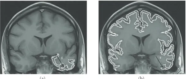
(a) (b)
Figure2: An MR-T1 image of the brain with one seedsinside the cortex. (a-b) The maximum influence zones ofswithin the cortex forfmax withδ3and withδ6, respectively. The asymmetry ofδ6favors segmentation in anticlockwise orientation, increasing the influence zone ofs.
reduces this problem, and in the case of seed competition, one can also replace δ3 by δ4 in (6). The basic idea in
function δ6 stemmed from [30], where the intensities on
the left and right sides of each arc are used to compute its weight, such that longer boundary segments are favored in only one orientation (either clockwise or anticlockwise). We are extending this idea to provide oriented region growing. Functionδ6is suitable to objects, such as the cortex,
composed by intermediary intensities with respect to the intensities on both of its sides. For MR-T1 images of the brain, the GM intensities in the cortex are expected to be higher than the intensities in one side (CSF) and lower than the intensities in the other side (WM). To grow regions in anticlockwise, we expect that the intensity Er(p,q) at a
distancerto the left (WM) of an arc (p,q) be higher than the intensityDr(p,q) at the same distancer to the right (CSF)
of the arc. We favor or penalize the arc dissimilarities based on this rule inδ6. The termg(p,q)·η(p,q) also penalizes
arcs which cross boundaries. The result is that the same seedsallows to delineate more pixels in the cortex withδ6
(Figure 2(b)), following the anticlockwise orientation, than withδ3(Figure 2(a)). Other interesting ideas of dissimilarity
functions for fmaxare presented in [11,19,23,31,32].
The basic differences between the formulations proposed in [11, 19, 20] are that (i) the former assumes δ(p,q) = δ(q,p) for all (p,q) ∈ A, and requires smooth path-cost functions, and (ii) the later allows asymmetric dissimilarity relations (e.g.,δ2), and nonsmooth cost functions (e.g., fmax
withδ3and seed competition). The strength of
connected-ness between image pixels in (i) is a symmetric relation, while it may be asymmetric in (ii). The main theoretical differences between our formulation and these ones are presented next.
3.1. Object definition without seed competition
We say that a pixel pisκ-connectedto a seeds∈S, if there exists an optimum pathπ fromsto psuch that f(π) ≤κ. Thisκ-connectivity relation will be asymmetric whenever the dissimilarityδ(p,q) is asymmetric.
Anobject is a maximal subset of DI wherein all pixels
p are at least κ-connected to one pixel s ∈ S. Similarly to the method presented in [23], the object is the union of all κ-connected components with respect to each seed s ∈ S,
which must be computed separately. This makesfmaxsmooth
for all dissimilarity functions described in (2)–(7).
The algorithm described in [23] assumes that the object can be defined by a single value of κ for all seeds in S. Figure 3(a) illustrates an example where this assumption works. However, a simple change in the position of a seed can fail segmentation (Figure 3(b)), because the influence zone of each seed inside the object is actually limited by a distinct value of costκ(Figure 3(c)). Moreover, the choice of seeds with distinct values ofκ usually reduces the number of seeds required to complete segmentation. This situation is better understood when we relate the concepts of minimum-spanning tree and minimum-cost path tree for fmax and
symmetricκ-connectivity relations [33].
Aminimum-spanning treeis a spanning forestP with a single arbitrary root, where the sum of the arc weightsδ(p,q) for all pairs (p,q) ∈ A, such thatP(q) = p, is minimum, as compared to any other minimum-spanning tree obtained from the original graph (DI,A) (Figures4(a)and4(b)). If we
remove the orientation of the arcs inFigure 4(b), every pair of pixels inPis connected by a path which is also optimum according to fmax (Figure 4(c)). That is, the
minimum-spanning tree encodes all possible minimum-cost path trees for fmax. Aκ-connected object with respect to a seedscan
be obtained by taking the component connected tos, after removing all arcs fromP whose δ(p,q) > κ. Suppose, for example, that the object is the brighter rectangle in the center ofFigure 4(a).Figure 4(c)shows that only the left side of the rectangle is obtained withs1andκ1=3. Ifκ1=4,s1reaches
the right side of the rectangle but invades the background. The rectangle can be obtained with three seeds andκ = 2. However, different values ofκreduce the number of seeds to two,s1withκ1=3 ands2withκ2=2 (Figure 4(d)).
s1
s2
(a)
s1
s2
(b)
s1
s2
(c)
Figure3: A CT image of a knee where the patella can be segmented with two seed pixels,s1ands2,fmaxwithδ3, and without seed competition. (a) The result with a single value ofκfor both seeds. (b) The segmentation with a single value ofκfails when we change the position ofs1, becauses1requires a higher value ofκto get the brighter part of the bone, andBinvades the background at this higher value ofκ. (c) The result can be corrected with distinct values ofκfor each seed.
1 2 1 0 1 2
1 8 8 4 6 3
1 5 5 9 7 3
0 1 0 3 3 1
(a)
1 1 1 1 1 1
0 0 0 4 2 3
0 3 0 2 1 0
1 1 1 0 2 2
(b)
s1
3 0
0 0
1
1 1 0
0
2 0 1 2
3
2 1 1 1 1 1 1
4 2
(c)
s1
s2 2 3
0
0 0
0
1
1 1 0 2
0 1 2
2
1 1 1 1 1
1
(d)
Figure4: (a) An image graph with 4-adjacency, where the integers are the image valuesI(p) and the bigger dot is an arbitrary pixel. The object of interest is the brighter rectangle in the center. (b) A minimum-spanning tree computed from the arbitrary pixel, where the integers for each pixelqare the arc weightsδ(p,q)= |I(q)−I(p)|, forp=P(q). (c) The minimum-spanning tree without arc orientation. A single seeds1can not extract the rectangle for any value ofκ. (d) The rectangle can be obtained with two seeds and distinct values ofκ,s1with κ1=3 ands2withκ2=2.
3.2. Object definition with seed competition
In [11,19], seeds are selected inside and outside the object, and theobject is defined by the subset of pixels which are more strongly connected to its internal seeds than to any other. This is the same as removing the arcs of maximum weight from the paths that connect object and background in the minimum-spanning tree. For example, the rectangle in Figure 4(c) is obtained by changing the position of s1
to any pixel in the background and selecting s2 as shown
inFigure 4(d). The main motivation for this paradigm was to eliminate the choice of κ, favoring the simultaneous segmentation of multiple objects.
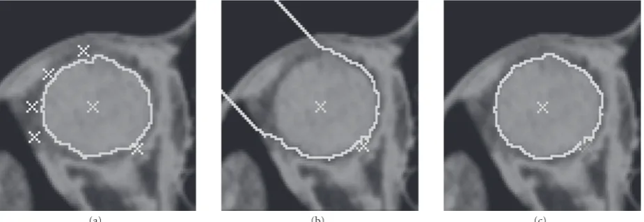
(a) (b) (c)
Figure5: A CT image of the orbital region where the eye ball is obtained by seed competition. (a) One internal seed and many external seeds are required for segmentation, usingfmaxwithδ4. (b) The segmentation fails when some of the external seeds are removed. (c) A value ofκ is used to limit the influence zone of the internal seed in parts, where the seed competition fails.
by the seed whose path cost is minimum. Note that even the internal seeds compete among themselves, and a distinct value of κ may be required for each seed. When the seed competition fails, these thresholds should limit the influence zones of the seeds avoiding connection between object and background, and the pixels, which are not conquered by any seed, should be considered as belonging to the background.
In general, the use of distinct values ofκ together with seed competition reduces the number of seeds required to complete segmentation.Figure 5(a)shows an example where many seeds have to be carefully selected in the background to delineate the object. The segmentation fails when some of these seeds are removed (Figure 5(b)), but it works when we limit the extent of the internal seed to some value ofκ (Figure 5(c)).
The algorithms and the problem of determining these thresholds for the internal seeds are addressed next.
4. ALGORITHMS
The IFT uses a variant of Dijkstra’s algorithm [34] to compute three attributes for each pixel p ∈ DI [21]: its
predecessorP(p) in the optimum path, the costC(p) of that path, and the corresponding root R(p). In the algorithms presented in this section, we do not need to create the predecessor mapP and the root mapRis only used in the case of seed competition.
The IFT with fmax propagates wavefrontsWcst of same
cost cst around each seed, following the order of the costs cst=0, 1,. . .,K. By assigning higher values ofδ(p,q) to arcs that cross the object’s boundary, the wavefronts fill first the object and, when they leak to the background, a considerable increase in their areas can be observed (Figures 6(a) and 6(b)). That is, many pixels in the background are reached by optimum paths whose cost is the lowest value δ(p,q) among the dissimilarities of the arcs (p,q) that cross the boundary. This ordered region growing process is exploited to compute the valuesκsof each seeds∈Sautomatically and
interactively.
4.1. Automatic computation ofκs
First consider the wavefronts around a seedsselected inside a given object. All pixels p in the wavefront Wcst around
s have optimum cost C(p) = cst, 0 ≤ cst ≤ K. If the object is a singleκ-connected component with respect tos, then there exists a thresholdκs, 0 ≤ κs ≤K, such that the
object can be defined by the union of all wavefrontsWcst, for
cst=0, 1,. . .,κs. We can specify a fixedκsfor this particular
application, but this is susceptible to intensity variations. Another alternative is to search for matchings between the shape of the object and the shape of the wavefronts. One drawback is the speed of segmentation, but this may be justified in some applications. A more complex situation occurs when the object definition requires more than one seed pixel. Each seed defines its own maximal extent inside the object and we need to match the shape of the object with the shape of the union of their influence zones.
The approach presented here is much simpler and yet effective. It stems from the previously mentioned observa-tion about the areas of the wavefronts, when they invade the background. The ordered region growing process of a seeds must stop when the size of its wavefront of cost cst is greater than an area threshold 0%< T <100%, computed over the image size, and the value ofκsis determined as max{cst−
1, 0}. The choice of one valueκsfor each seeds ∈Sis then
substituted by the choice ofT, which limits the maximum sizes of the wavefronts. This threshold can be verified by selecting internal seeds and settingT =99%. The total area of the wavefronts during propagation can be displayed as a curve. A peak on this curve indicates the maximum possible value for T at the instant of leaking. Some animations of this ordered region growing process are provided inhttp:// www.liv.ic.unicamp.br/demo/miranda-kconnected.avi.
The algorithms are presented for single object delin-eation without seed competition (Algorithm 1) and multiple object definition with seed competition (Algorithm 2).
INPUT: ImageI=(DI,I), adjacencyA, internal seedsS, and path-cost functionfmax, and the size thresholdT. OUTPUT: Binary imageL=(DI,L), whereL(p)=1, ifpbelongs to the object, andL(p)=0 otherwise.
Auxiliary: A priority queueQ, variables tmp,κ, cst and size, and cost mapCdefined inDI.
(1) For every pixelp∈DI, setL(p)←0.
(2) WhileS /=∅, do
(3) For every pixelp∈DI, setC(p)←+∞.
(4) Remove a seedsfromS.
(5) SetC(s)←0, size←0, cst←0,κ←+∞, and insertsinQ. (6) WhileQ /=∅andκ=+∞, do
(7) Remove a pixelpfromQsuch thatC(p) is minimum. (8) For everyq∈A(p), such thatC(q)> C(p), do (9) Set tmp←max{C(p),δ(p,q)}.
(10) If tmp< C(q), then
(11) IfC(q)=/ +∞, then removeqfromQ. (12) SetC(q)←tmp and insertqinQ. (13) IfC(p)=/cst, then set size←1 and cst←C(p). (14) Else, set size←size + 1.
(15) If size> Tthen setκ←max{cst−1, 0} (16) For every pixelp∈DI, do
(17) IfC(p)≤κ, then setL(p)←1. (18) Remove any remaining pixels fromQ.
Algorithm1: Single object definition without seed competition.
Input: ImageI=(DI,I), adjacencyA, path-cost functionfmax, size thresholdT, and a labeled imageL=(DI,L),
whereL(p)=i, 0≤i≤k, ifpis a seed pixel selected inside objecti >0 amongkobjects, beingi=0 reserved for seeds in the background, andL(p)= −1 otherwise.
Output: A labeled imageL=(DI,L), whereL(p)=i, 0≤i≤k.
Auxiliary: Priority queueQ, variable tmp, andC,R,κ, size, and cst are maps defined inDIto store cost and root
of each pixel and threshold, wavefront size, and wavefront cost of each seed, respectively.
(1) For every pixelp∈DI, do
(2) SetR(p)←p, size(p)←0, cst(p)←0, andκ(p)←+∞. (3) IfL(p)= −1, then setC(p)←+∞andL(p)←0. (4) Else, setC(p)←0 and insertpinQ.
(5) WhileQ /=∅, do
(6) Remove a pixelpfromQsuch thatC(p) is minimum. (7) Ifκ(R(p))=+∞andL(R(p))=/0, then
(8) IfC(p)=/ cst(R(p)), then set size(R(p))←1 and cst(R(p))←C(p). (9) Else, set size(R(p))←size(R(p)) + 1.
(10) If size(R(p))> T, then setκ(R(p))←max{cst(R(p))−1, 0}. (11) IfC(p)≤κ(R(p)), then
(12) For everyq∈A(p), such thatC(q)> C(p), do (13) Set tmp←max{C(p),δ(p,q)}.
(14) If tmp< C(q), then
(15) IfC(q)=/ +∞, then removeqfromQ.
(16) SetC(q)←tmp,R(q)←R(p), and insertqinQ. (17) For every pixelp∈DI, do
(18) IfC(p)≤κ(R(p)), then setL(p)←L(R(p)).
Algorithm2: Multiple object definition with seed competition.
algorithm stops propagation when the value κs of a seeds
is found. In the case of seed competition, the root map is used to find in constant time the root of each pixel inS. The influence zone of a seeds∈Sis limited either when it meets
the influence zone of other seed at the same minimum cost or when the valueκsofsis found.
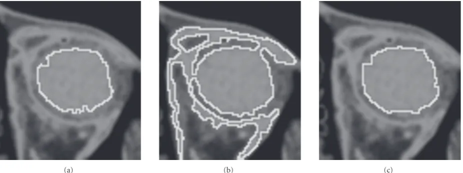
(a) (b) (c)
Figure6: A CT image of the orbital region with one seed inside the eye ball. (a) A wavefront of costκwhich represents the maximum extent of this seed inside the eye ball. (b) The wavefront of costκ+ 1 shows a considerable augment in size when it invades the background. (c) The pixel propagation order provides more continuous transitions of the wavefronts to selectκ, interactively.
A B
(a)
A B
(b)
A B
(c) (d)
Figure7: Segmentation of a caudate nucleus with two internal seeds,AandB. (a) The leaking occurs before the object be filled. (b) The moment whenκA=324 is detected. (c) The instant whenκBis detected. (d) Final segmentation.
occurs when the object contains several background parts (holes) inside it. In this case, the use ofκsusually eliminates
the need for at least one background seed at each hole. On the other hand, some small noisy parts of the object may not be conquered by the internal seeds due to the use ofκs.
The labeled image can be postprocessed, such that holes with area below a threshold are closed [37,38]. The area closing operator has shown to be a very effective complement for the presented algorithms. In many situations, the objects do not have holes and high area thresholds can be used to reduce the number of internal seeds.
The animations in http://www.liv.ic.unicamp.br/demo/ miranda-kconnected.aviwere created by usingAlgorithm 2. It is usually preferable with respect toAlgorithm 1, because it allows faster multiple object segmentation. Note that a wavefront of one seed can leak to the background before the object be fully filled by the wavefronts of other seeds. Figure 7(a)illustrates an example where the leaking occurs for seed A before the object be filled. The moment when κA=324 is detected is shown inFigure 7(b), andFigure 7(c)
shows the instant when κB = 770 is detected. The figures
show only a region of interest of the original image,
where the segmentation was done with T = 1%. The final segmentation is shown in Figure 7(d). Even when the dissimilarities are not higher for arcs that cross the object’s boundary,Algorithm 2 can work either due to the seed competition among internal seeds (parts of the object can be filled without leaking) or due to the automatic κs
computation, as shown in the example ofFigure 7.
4.2. Interactive computation ofκs
A first approach is to compute the IFT for every pixelp∈DI,
such that the cost C(p) of the optimum path that reaches p from S is found. In the case of seed competition, the corresponding root R(p) ∈ S is also propagated to each pixelp∈DI. Then, the user moves the cursor of the mouse
over the image, and for each position q of the cursor, the program displays the influence zone of the corresponding root s = R(q) ∈ S defined by pixels p ∈ DI, such that
C(p)≤C(q) andR(p)=R(q). This interactive process can be repeated until the user selects a pixel q to confirm the influence zone ofs(i.e.,κs=C(q)). The user can repeat this
Input: ImageI=(DI,I), adjacencyA, internal seedsS, and path-cost functionfmax.
Output: Binary imageL=(DI,L), whereL(p)=1, ifpbelongs to the object, andL(p)=0 otherwise.
Auxiliary: Priority queueQ, variables tmp, ord, and cost mapCand propagation order mapOdefined inDI.
(1) For every pixelp∈DI, setL(p)←0.
(2) WhileS /=∅, do
(3) For every pixelp∈DI, setC(p)←+∞.
(4) Remove a seedsfromS.
(5) SetC(s)← 0, ord←0, and insertsinQ. (6) WhileQ /=∅, do
(7) Remove a pixelpfromQsuch thatC(p) is minimum. (8) SetO(p)←ord + 1 and ord←ord + 1.
(9) For everyq∈A(p), such thatC(q)> C(p), do (10) Set tmp←max{C(p),δ(p,q)}.
(11) If tmp< C(q), then
(12) IfC(q)=/ +∞, then removeqfromQ. (13) SetC(q)←tmp and insertqinQ. (14) The user selects a pixelqon the image.
(15) For every pixelp∈DI, do
(16) IfO(p)≤O(q), then setL(p)←1.
Algorithm3: Single object definition without seed competition.
One drawback of the method above is the abrupt size variations of the wavefronts (Figures6(a)and6(b)), which makes the selection of pixel q sometimes difficult. We circumvent the problem by exploiting thepropagation order O(p) (a number from 1 to |DI|) of each pixel p removed
from Q during execution of the IFT. Note that a pixel p propagates before a pixelq (i.e.,O(p) < O(q)) when it is reached by an optimum path from S, whose cost C(p) is less than the costC(q) of the optimum path that reachesq. WhenC(p)=C(q), we assume afirst-in-first-out(FIFO) tie-breaking policy forQ. That is, among all pixels with the same minimum cost in Q, the one first reached by an optimum path fromSis removed for propagation. Therefore, we also compute the propagation orderO(p) of each pixel p ∈DI.
When the user moves the cursor to a positionq, the program displays the influence zone of the corresponding root s = R(q)∈Sdefined by pixels p ∈DI, such thatO(p)≤O(q)
andR(p)= R(q). The rest of the process is the same. Note that althoughκs =C(q), only the pixels pin the wavefront
WC(q)which haveO(p)≤O(q) are selected as belonging to
the influence zone ofs. This provides smoother transitions between consecutive wavefronts (Figure 6(c)) as compared to the first idea. See Algorithms3and4.
5. EVALUATION
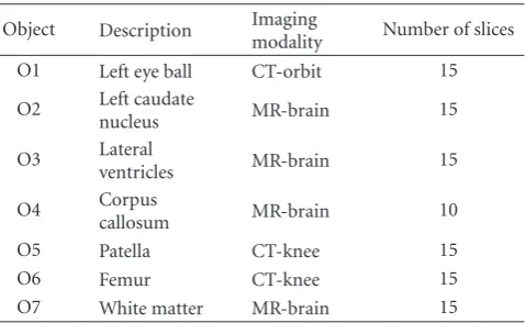
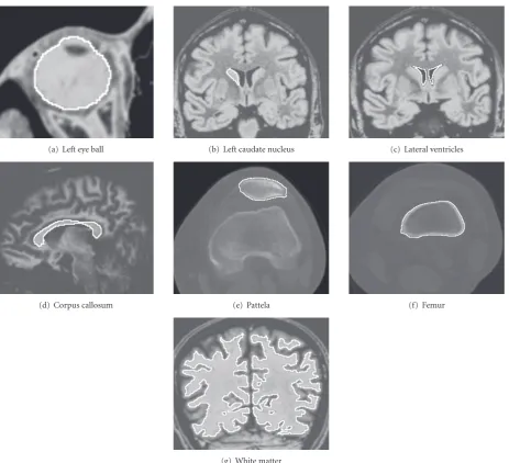
We have selected 100 images from magnetic resonance (MR) and computerized tomography (CT) data sets of 7 objects for evaluation (seeTable 1andFigure 8). Each object consists of some slices that represent different degrees of challenge for segmentation. The original images have been preprocessed to increase the similarities between pixels inside the objects and the contrast between object and background. Each of four
Table1: Description, imaging modality, and number of slices for each object used in the experiments.
Object Description Imaging
modality Number of slices
O1 Left eye ball CT-orbit 15
O2 Left caudate
nucleus MR-brain 15
O3 Lateral
ventricles MR-brain 15
O4 Corpus
callosum MR-brain 10
O5 Patella CT-knee 15
O6 Femur CT-knee 15
O7 White matter MR-brain 15
users has performed segmentation over the 100 images using each of three methods, M1, M2, and M3, with interactive seed selection (mouse clicks).
M1: Object delineation without seed competition and automatic/interactive computation of κs. This
method uses Algorithms1and3. When M1 requires a singleκsfor all seeds, it indicates that absolute-fuzzy
connectedness (AFC) would work.
M2: Object delineation with seed competition and auto-matic κs computation. This method uses only
Algorithm 2. We did not evaluate Algorithm 4, because preliminary tests indicated that user inter-vention to add external seeds in Algorithm 2 is simpler and more effective than to indicate κs in
(a) Left eye ball (b) Left caudate nucleus (c) Lateral ventricles
(d) Corpus callosum (e) Pattela (f) Femur
(g) White matter
Figure8: (a)–(g) Results of slice segmentation of the objects from 1 to 7, respectively, overlaid with the preprocessed images.
M3: Object delineation with seed competition without κscomputation. As mentioned inSection 1,
relative-fuzzy connectedness (RFC) and watershed transform by markers (WT) are the same method [22] (one is the dual of the other), represented here by M3.
Therefore, the user can correct segmentation by adding/removing seeds in M1, M2, and M3, and in the case of M1, by pointing the mouse to the pixel, whose propaga-tion order indicates the correctκsimplicitly (Section 4.2).
M1 aims to show two aspects about AFC: (i) a singleκfor all seeds is not sufficient in most cases and (ii) the problem of computing multipleκsthresholds can be easily solved by a
wavefront area threshold 0% < T < 100%, computed over the image size. Note that, being M1 an extension of AFC, there is no situation where AFC works and M1 would fail. M2 aims to reduce the number of required seeds with respect to M3 by automaticκscomputation. When this automatic
procedure fails, M2 becomes M3. Therefore, in the worst case, the efficiency of M2 should be the same of M3.
Given that M1 and M2 are extensions of AFC and RFC/WT, we expect that they do not affect the accuracy of the original approaches, which is assumed to be good from the results of several other works [10,14–18]. The experiments then aimed to show that M1 works in situations where AFC would fail, M1 and M2 require less user interaction than M3, and the methods produce similar results.
Input: ImageI=(DI,I), adjacencyA, path-cost functionfmax, and a labeled imageL=(DI,L), whereL(p)=i,
0≤i≤k, ifpis a seed pixel selected inside objecti > 0 fromkobjects, beingi=0 reserved for seeds in the background, andL(p)= −1 otherwise.
Output: A labeled imageL=(DI,L), whereL(p)=i, 0≤i≤k.
Auxiliary: Priority queueQ, variables tmp and ord, andC,R,Oare maps defined inDI to store cost, root and
propagation order of each pixel, respectively.
(1) Set ord←0.
(2) For every pixelp∈DI, do
(3) SetR(p)←p.
(4) IfL(p)= −1, then setC(p)←+∞andL(p)←0. (5) Else, setC(p)←0 and insertpinQ.
(6) WhileQ /=∅, do
(7) Remove a pixelpfromQsuch thatC(p) is minimum. (8) SetO(p)←ord + 1 and ord←ord + 1.
(9) For everyq∈A(p), such thatC(q)> C(p), do (10) Set tmp←max{C(p),δ(p,q)}.
(11) If tmp< C(q), then
(12) IfC(q)=/ +∞, then removeqfromQ.
(13) SetC(q)←tmp,R(q)←R(p), and insertqinQ. (14) While the user is not satisfied.
(15) The user can select a pixelqon the image. (16) For every pixelp∈DI, do
(17) IfO(p)≤O(q) andR(p)=R(q), then setL(p)←L(R(p)).
Algorithm4: Multiple object definition with seed competition.
Table2: The dissimilarity functions used for each combination of object and method.
Object M1 M2 M3
O1 δ3 δ2 δ2
O2 δ3 δ4 δ2
O3 δ3 δ3 δ3
O4 δ3 δ4 δ2
O5 δ3 δ4 δ4
O6 δ3 δ3 δ2
O7 δ3 δ3 δ3
M2). Since objects from O1 to O6 do not have holes, we set the area closing threshold to some arbitrary high value (e.g., 500 pixels). The only exception was O7, whose area closing threshold could not be higher than 3 pixels due to its holes. In functionδ2, we used the magnitude of the Sobel’s gradient.
The value ofσwas 20 for all cases involvingδ3andδ4. Note
also thatδ3has been chosen in some situations involving seed
competition, despite fmaxis not smooth.
Each object was represented by a set ofl binary slices
Li=(DI,Li),i=1, 2,. . .,l, whereLi(p)=1 for object pixels
and 0 otherwise. LetLiandLibe the binary images resulting
from the segmentation of a same object slice using different methods. The similarity between these results was measured by
1.0−
i=l i=1
∀p∈DILi(p)⊕Li(p) i=l
i=1
∀p∈DILi(p) + i=l
i=1
∀p∈DILi(p) , (8)
where⊕is the “exclusive or” operation (i.e.,Li(p)⊕Li(p)=
1, ifLi(p)=/ Li(p), and 0 otherwise). Given that we have four
different users using three distinct methods, we may assume that similarity values around 0.90 represent good agreement in delineation (Figure 9).
The number of user interactions in M3 is the total number of seeds selected inside (NIS—number of internal seeds) and outside (NES—number of external seeds) the object. In M1, the amount of user interaction is represented by the total number of interactive κs detections(IKD) and
NIS. The automatic κs detections (AKD) are chosen as
much as possible in order to reduce the number of user interactions. In M2, the number of user interactions is computed as in M3, but the number of seeds is expected to be much less due to automaticκsdetection.
Instead of quantifying the number of user interactions for a fixed value ofκ, we decided to quantify the number of differentκsvalues found in M1 for cases of multiple seeds.
Thepercentages of differentκsvalues(PDK) are presented in
Table 3, together with the average number of interactions and similarity values among all users. Note that O3 was detected with a same value of κ, but the other objects required from 6.8% to 92.4% of differentκsvalues. O5 did
(a) (b)
Figure9: (a) A segmentation of the left caudate nucleus. (b) The result of dilating the binary image with a circular structuring element of radius 1. The similarity value between these two masks is 0.87. The differences in the experiments using distinct methods on this object (O2) are less significant than this small dilation.
Table3: The percentages of differentκsvalues (PDK) in M1, the average numbers of user interactions for each object and method, and the
average similarity values between different methods for a same object.
M1 PDK M2 M3 M1, M2 M1, M3 M2,M3
O1 35.0 83.4% 29.5 77.6 0.965 0.969 0.962
O2 38.5 92.4% 29.3 38.8 0.904 0.890 0.915
O3 31.8 0.0% 31.3 61.3 0.992 0.932 0.935
O4 29.7 57.4% 27.5 46.8 0.922 0.914 0.918
O5 15.0 — 15.0 61.0 0.973 0.954 0.946
O6 26.3 27.1% 26.3 37.8 0.992 0.982 0.981
O7 47.5 6.8% 46.3 284.8 0.973 0.931 0.930
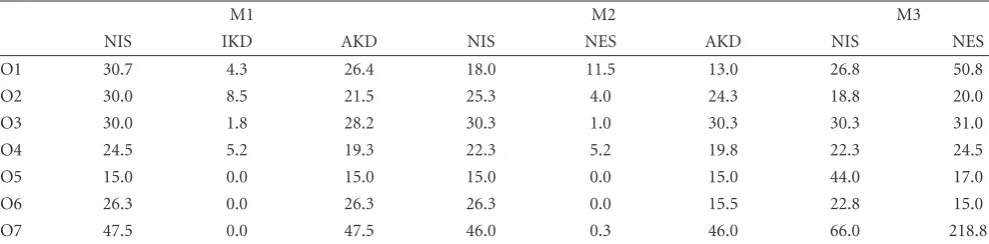
Table4: Average numbers of internal seeds (NIS), interactiveκsdetections (IKD), external seeds (NES), and automaticκsdetections (AKD).
M1 M2 M3
NIS IKD AKD NIS NES AKD NIS NES
O1 30.7 4.3 26.4 18.0 11.5 13.0 26.8 50.8
O2 30.0 8.5 21.5 25.3 4.0 24.3 18.8 20.0
O3 30.0 1.8 28.2 30.3 1.0 30.3 30.3 31.0
O4 24.5 5.2 19.3 22.3 5.2 19.8 22.3 24.5
O5 15.0 0.0 15.0 15.0 0.0 15.0 44.0 17.0
O6 26.3 0.0 26.3 26.3 0.0 15.5 22.8 15.0
O7 47.5 0.0 47.5 46.0 0.3 46.0 66.0 218.8
performances of M1 and M2 have been equivalent, M2 is preferable because its extension to 3D does not suffer from interactive κs indication and it can provide simultaneous
segmentation of multiple objects.
Table 4shows in detail the average values of NIS, NES, IKD, and AKD for each object and method. Note that, AKD varied from 59% to 100% of NIS, being on average 90% of NIS in M1 and 88% of NIS in M2. This demonstrates the effectiveness of the proposed approach for automaticκs
detection and explains the reduction of user interactions in M1 and M2 with respect to M3. Note also that the number of external seeds was considerably reduced in comparison to M3. This is an important result for future automation, because seed competition is sensitive to the location of the external seeds due to the heterogeneity of the background.
6. CONCLUSIONS
We have presented four IFT-based algorithms for object delineation based on κ-connected components with and without seed competition. They differ from the previous approaches in the following aspects: computation of different values of κ for each seed, effective automatic κs detection,
and user friendlyκscomputation, where the user moves the
these results are extensive to other image types by suitable choice of pre-processing and dissimilarity function.
The interactive κs detection counted with real time
response for every position of the cursor, but this may not be feasible in 3D segmentation involving several slices. In this sense, the algorithms based on interactiveκs detection
are more adequate for 2D/3D segmentation in a slice by slice fashion, where seeds may be automatically propagated along the slices. In such a case, the interactiveκsdetection can be
used to correct segmentation when the automatic detection ofκsfails.
Seed competition with automatic κs detection
(Algorithm 2) seems to be the most promising approach. We are currently investigating two approaches for 3D segmentation of medical images: (i) automatic segmentation with only internal seeds and automaticκsdetection, and (ii)
interactive segmentation with automaticκsdetection, where
the user can add/remove internal and external seeds, and subsequent IFTs are executed in a differential way [27].
ACKNOWLEDGMENTS
The authors thank FAPESP (Procs. 05/59808-0, 05/58103-3, 05/56578-4, and 03/13424-1), CNPq (Procs. 302617/2007-8 and 472402/2007-2), and CAPES for the financial support. Furthermore, the authors thank the reviewers and editors for their contributions.
REFERENCES
[1] M. Kass, A. Witkin, and D. Terzopoulos, “Snakes: active contour models,” International Journal of Computer Vision, vol. 1, no. 4, pp. 321–331, 1988.
[2] T. F. Cootes, C. J. Taylor, D. H. Cooper, and J. Graham, “Active shape models—their training and application,” Computer Vision and Image Understanding, vol. 61, no. 1, pp. 38–59, 1995.
[3] T. Cootes, G. Edwards, and C. J. Taylor, “Active appearance models,” in Proceedings of the 5th European Conference on Computer Vision (ECCV ’98), vol. 2, pp. 484–498, Freiburg, Germany, June 1998.
[4] P. Viola and M. Jones, “Rapid object detection using a boosted cascade of simple features,” in Proceedings of IEEE Computer Society Conference on Computer Vision and Pattern Recognition (CVPR ’01), vol. 1, pp. 511–518, Kauai, Hawaii, USA, December 2001.
[5] J. Shi and J. Malik, “Normalized cuts and image segmen-tation,”IEEE Transactions on Pattern Analysis and Machine Intelligence, vol. 22, no. 8, pp. 888–905, 2000.
[6] Y. Y. Boykov and M.-P. Jolly, “Interactive graph cuts for optimal boundary & region segmentation of objects in N-D images,” in Proceedings of the 8th IEEE International Conference on Computer Vision (ICCV ’01), vol. 1, pp. 105– 112, Vancouver, Canada, July 2001.
[7] V. Kolmogorov and R. Zabih, “What energy functions can be minimized via graph cuts?”IEEE Transactions on Pattern Analysis and Machine Intelligence, vol. 26, no. 2, pp. 147–159, 2004.
[8] Y. Boykov and V. Kolmogorov, “An experimental comparison of min-cut/max-flow algorithms for energy minimization in vision,” IEEE Transactions on Pattern Analysis and Machine Intelligence, vol. 26, no. 9, pp. 1124–1137, 2004.
[9] S. Wang and J. M. Siskind, “Image segmentation with mini-mum mean cut,” inProceedings of the 8th IEEE International Conference on Computer Vision (ICCV ’01), vol. 1, pp. 517– 524, Vancouver, Canada, July 2001.
[10] J. K. Udupa and P. K. Saha, “Fuzzy connectedness and image segmentation,” Proceedings of the IEEE, vol. 91, no. 10, pp. 1649–1669, 2003.
[11] P. K. Saha and J. K. Udupa, “Relative fuzzy connectedness among multiple objects: theory, algorithms, and applications in image segmentation,”Computer Vision and Image Under-standing, vol. 82, no. 1, pp. 42–56, 2001.
[12] L. Vincent and P. Soille, “Watersheds in digital spaces: an efficient algorithm based on immersion simulations,” IEEE Transactions on Pattern Analysis and Machine Intelligence, vol. 13, no. 6, pp. 583–598, 1991.
[13] S. Beucher and F. Meyer, “The morphological approach to segmentation: the watershed transformation,” in Mathemat-ical Morphology in Image Processing, chapter 12, pp. 433–481, Marcel Dekker, New York, NY, USA, 1993.
[14] T. Lei, J. K. Udupa, P. K. Saha, and D. Odhner, “Artery-vein separation via MRA-an image processing approach,”IEEE Transactions on Medical Imaging, vol. 20, no. 8, pp. 689–703, 2001.
[15] G. Moonis, J. Liu, J. K. Udupa, and D. B. Hackney, “Estimation of tumor volume with fuzzy-connectedness segmentation of MR images,”American Journal of Neuroradiology, vol. 23, no. 3, pp. 356–363, 2002.
[16] H. T. Nguyen, M. Worring, and R. van den Boomgaard, “Watersnakes: energy-driven watershed segmentation,”IEEE Transactions on Pattern Analysis and Machine Intelligence, vol. 25, no. 3, pp. 330–342, 2003.
[17] V. Grau, A. U. J. Mewes, M. Alca˜niz, R. Kikinis, and S. K. Warfield, “Improved watershed transform for medical image segmentation using prior information,”IEEE Transactions on Medical Imaging, vol. 23, no. 4, pp. 447–458, 2004.
[18] Y.-P. Tsai, C.-C. Lai, Y.-P. Hung, and Z.-C. Shih, “A Bayesian approach to video object segmentation via merging 3-D watershed volumes,”IEEE Transactions on Circuits and Systems for Video Technology, vol. 15, no. 1, pp. 175–180, 2005. [19] G. T. Herman and B. M. Carvalho, “Multiseeded segmentation
using fuzzy connectedness,” IEEE Transactions on Pattern Analysis and Machine Intelligence, vol. 23, no. 5, pp. 460–474, 2001.
[20] J. K. Udupa, P. K. Saha, and R. A. Lotufo, “Relative fuzzy connectedness and object definition: theory, algorithms, and applications in image segmentation,” IEEE Transactions on Pattern Analysis and Machine Intelligence, vol. 24, no. 11, pp. 1485–1500, 2002.
[21] A. X. Falc˜ao, J. Stolfi, and R. A. Lotufo, “The image foresting transform: theory, algorithms, and applications,”IEEE Trans-actions on Pattern Analysis and Machine Intelligence, vol. 26, no. 1, pp. 19–29, 2004.
[22] R. Audigier and R. A. Lotufo, “Seed-relative segmen-tation robustness of watershed and fuzzy connectedness approaches,” inProceedings of the 20th Brazilian Symposium on Computer Graphics and Image Processing (SIBGRAPI ’07), pp. 61–70, Minas Gerais, Brazil, October 2007.
[23] J. K. Udupa and S. Samarasekera, “Fuzzy connectedness and object definition: theory, algorithms, and applications in image segmentation,”Graphical Models and Image Processing, vol. 58, no. 3, pp. 246–261, 1996.
mentation with differential image foresting transforms,”IEEE Transactions on Medical Imaging, vol. 23, no. 9, pp. 1100–1108, 2004.
[28] A. X. Falc˜ao, F. P. G. Bergo, and P. A. V. Miranda, “Image segmentation by tree pruning,” in Proceedings of the 17th Brazilian Symposium of Computer Graphic and Image Process-ing (SIBGRAPI ’04), pp. 65–71, Curitiba, Brazil, October 2004. [29] P. K. Saha and J. K. Udupa, “Fuzzy connected object delin-eation: axiomatic path strength definition and the case of multiple seeds,” Computer Vision and Image Understanding, vol. 83, no. 3, pp. 275–295, 2001.
[30] A. X. Falc˜ao, J. K. Udupa, S. Samarasekera, S. Sharma, B. E. Hirsch, and R. A. Lotufo, “User-steered image segmentation paradigms: live wire and live lane,” Graphical Models and Image Processing, vol. 60, no. 4, pp. 233–260, 1998.
[31] P. K. Saha, J. K. Udupa, and D. Odhner, “Scale-based fuzzy connected image segmentation: theory, algorithms, and validation,”Computer Vision and Image Understanding, vol. 77, no. 2, pp. 145–174, 2000.
[32] P. K. Saha and J. K. Udupa, “Tensor scale-based fuzzy connectedness image segmentation,” inMedical Imaging 2003: Image Processing, vol. 5032 ofProceedings of SPIE, pp. 1580– 1590, San Diego, Calif, USA, February 2003.
[33] C. All`ene, J. Y. Audibert, M. Couprie, J. Cousty, and R. Keriven, “Some links between min-cuts, optimal spanning forests and watersheds,” inProceedings of the 8th International Symposium on Mathematical Morphology and Its Applications to Signal and Image Processing (ISMM ’07), pp. 253–264, Rio de Janeiro, Brazil, October 2007.
[34] E. W. Dijkstra, “A note on two problems in connexion with graphs,”Numerische Mathematik, vol. 1, no. 1, pp. 269–271, 1959.
[35] A. X. Falc˜ao, J. K. Udupa, and F. K. Miyazawa, “An ultra-fast user-steered image segmentation paradigm: live wire on the fly,”IEEE Transactions on Medical Imaging, vol. 19, no. 1, pp. 55–62, 2000.
[36] P. Felkel, M. Bruckschwaiger, and R. Wegenkittl, “Imple-mentation and complexity of the watershed-from-markers algorithm computed as a minimal cost forest,” Computer Graphics Forum, vol. 20, no. 3, pp. C26–C35, 2001.
[37] A. Meijster and M. H. F. Wilkinson, “A comparison of algorithms for connected set openings and closings,” IEEE Transactions on Pattern Analysis and Machine Intelligence, vol. 24, no. 4, pp. 484–494, 2002.