A new low-complexity angular spread estimator in the presence of line-of-sight with angular distribution selection

R E S E A R C H

Open Access

A new low-complexity angular spread estimator

in the presence of line-of-sight with angular

distribution selection

Inès Bousnina

, Alex Stéphenne

, Sofiène Affes

and Abdelaziz Samet

Abstract

This article treats the problem of angular spread (AS) estimation at a base station of a macro-cellular system when a line-of-sight (LOS) is potentially present. The new low-complexity AS estimator first estimates the LOS component with a moment-basedK-factor estimator. Then, it uses a look-up table (LUT) approach to estimate the mean angle of arrival (AoA) and AS. Provided that the antenna geometry allows it, the new algorithm can also benefit from a new procedure that selects the angular distribution of the received signal from a set of possible candidates. For this purpose, a nonlinear antenna configuration is required. When the angular distribution is known, any antenna structure could be used a priori; hence, we opt in this case for the simple uniform linear array (ULA). We also compare the new estimator with other low-complexity estimators, first with Spread Root-MUSIC, after we extend its applicability to nonlinear antenna array structures, then, with a recently proposed two-stage algorithm. The new AS estimator is shown, via simulations, to exhibit lower estimation error for the mean AoA and AS estimation.

Keywords:angular spread, mean angle of arrival, angular distribution selection, look-up table, extended spread root-MUSIC

I. Introduction

Smart antennas will play a major role in future wireless communications. There exist several smart antenna techniques such as beamforming, antenna diversity, and spatial multiplexing. Future smart antennas will most likely switch from one technique to another according to the channel parameters [1]. One of the most impor-tant parameters is the multipath angular spread (AS). For instance, the beamforming technique is to be con-sidered when the AS is relatively small, while antenna diversity is more appropriate in other cases. Moreover, mean angle of arrival (AoA) and AS estimates are required to locate the mobile station [2].

In the last two decades, several algorithms have been developed for the direction of arrival and AS estimation. Based on the concept of generalization of the signal and noise subspaces, 3 multiple signal classification (MUSIC) is the most known mean AoA estimator. For AS estima-tion, many derivatives have been proposed. DSPE [3]

and DISPARE [4] are two generalizations of the MUSIC algorithm for distributed sources. They involve maxi-mizing cost functions that depend on the noise eigen-vectors. The mentioned estimators are computationally heavy because of the required multi-dimensional sys-tems resolution. A low-complexity subspace-based method, Spread Root-MUSIC, is presented in [5] where a rank-two model is fitted at each source, using the standard point source direction of arrival algorithm Root-MUSIC. This rank-two model depends indirectly on the parameters that can be estimated using a simple look-up table (LUT) procedure. In [6], a generalized Weighted Subspace Fitting algorithm is proposed. The latter, in contrast to DSPE and DISPARE, gives consis-tent estimates for a general class of full-rank data mod-els. In [7], a subspace-based algorithm has been formulated that is applicable to the case of incoherently distributed multiple sources. In this algorithm, the total least squares (TLS) estimation of signal parameters via rotational invariance techniques (TLS-ESPRIT) approach is employed to estimate the source mean AoA. Then, the AS is estimated using the LS covariance matrix

* Correspondence: [email protected]

1_{Tunisian Polytechnic School, B.P. 743-2078, La Marsa, Tunisia} Full list of author information is available at the end of the article

fitting. However, the performance of this algorithm shows unsatisfactory results under some practical condi-tions [8]. In [9], a maximum likelihood (ML) algorithm has been proposed for the localization of Gaussian dis-tributed sources. The likelihood function is jointly maxi-mized for all parameters of the Gaussian model. It requires the resolution of a four-dimensional (4D) non-linear optimization problem. In [9] and [10], LS algo-rithms are considered to reduce the dimension of the system. The simplified ML algorithm belongs to the covariance matching estimation techniques (COMET) [11]. In [12], a low-complexity algorithm based on the concept of contrast of eigenvalues (COE) has been developed to estimate AS and mean AoA. The authors establish a bijective relationship between the COE of the covariance matrix: the signal-to-noise ratio (SNR) value and the value of the AS. Hence, for each SNR, a LUT is built. The mean AoA is derived using the estimated AS and the number of dominant eigenvalues of the source covariance matrix.

Many of these estimators make assumptions on the shape of the signal distribution, assume narrow spatial spreads, and eigen-decompose the full-rank covariance matrix into a signal subspace and a pseudo-noise subspace. Most often they result into a multi-dimensional optimization problem, implying high com-putational loads.

To overcome this limitation, a low-complexity estima-tor [5] has been developed. Spread Root-MUSIC con-sists in a 2D search using the Root-MUSIC algorithm. Another mean AoA and AS estimator based on the same approach as Spread Root-MUSIC was developed in [13]. Indeed, thanks to Taylor series expansions, the estimation of AoA and AS is transformed into a locali-zation of two closely, equi-powered and uncorrelated rays. However, like other estimators, Spread Root-MUSIC considers scenarios without line-of-sight (LOS). A new low-complexity estimator, based on a LUT approach was therefore developed [14]. First, it esti-mates the LOS component of the Rician correlation coefficient and deduces the Non-LOS (NLOS) compo-nent. Then, it extracts the desired parameters from LUTs computed off-line. The new estimator, like most estimators, assumes the a priori knowledge of the angu-lar distribution of the received signal. In this article, we enable this method to select the angular distribution type from a set of possible candidates. For this purpose, a nonlinear array structure is required. We also compare the new technique to other low-complexity AS estima-tors. The first one is derived by extending the Spread Root-MUSIC algorithm [5] to the considered antenna configuration. The second one is the two-stage approach developed in [13].

The article is organized as follows. In Section 2, we def ne the used notations and describe the data model. In Section 3, we describe the new method for selecting the angular distribution type. Section 4 details the two low-complexity AS estimation methods that will be used to benchmark our newly proposed approach, that is the Spread Root-MUSIC algorithm [5], modified to handle a nonlinear array structure, and the two-stage approach presented in [13]. In Section 5, simulation 5 results are presented and discussed.

II. Notations and data model

In this article, non-bold letters denote scalars. Lowercase bold letters represent vectors. Uppercase bold letters represent matrices. The row-column notation is used for the subscripts of matrix elements. For example,Ris a matrix andRikis the element of that matrix on theith row and thekth column. The sign∧_.denotes an esti-mate. Superscripts between parenthesis are used to dif-ferentiate estimates at different stages of the estimation process.

In this article, we consider the single input-multiple output (SIMO) model for the uplink (mobile to base station) transmission. The mobile has a single isotropic antenna surrounded by scatterers. We also assume that the base station is located high enough and far from the mobile to ensure 2D AoAs and to avoid local scattering shadowing. As one example, these conditions are observed in the current GSM and 3G networks where the base station is usually placed on the building roofs. As in [14,5,15,7], we suppose that the base station antenna-elements are isotropic and that the same mean AoA and AS are seen at all antenna-elements of the base station.

We consider the estimation of the AS and mean AoA from estimates over time of the time-varying channel coefficients associated with a single time-differentiable path at the multiple elements of an antenna array. Our model can therefore be associated with a narrowband channel, or with a given time-differentiable path of a wideband channel. Of course, in a wideband channel scenario, the potential presence of a LOS would only be considered for the first time-differentiable path, and knowledge of a zeroK-factor could be assumed for the rest of the paths. We consider the following expression for the Rician channel coefficient [16]:

¯

xi(t) =

K+ 1ai(t) +

K

K+ 1exp

j2πFdcos(γd)t+j2π d0i

λ sin(θ0i)

, (1)

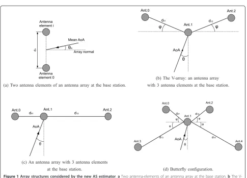
frequency and Doppler angle. lis the wavelength and d0i is the distance between the antenna reference and the antenna-element i, andθ0iis the AoA of the LOS, as shown in Figure 1a. Indeed, in our model, we con-sider uniform clusters, so that the mean AoA corre-sponds to the AoA of the LOS. Letxibe

xi= [xi(0)· · ·xi(N−1)], (2) wherexi(n) =x¯i(nTs), andTsis the sampling interval. In this study, we consider an arbitrary array geometry. That is why the array model described for instance in [3] and [11] is not adopted herea. Instead, we use the correlation coefficient of the Rician channel coefficients received at the antenna branch (i, k) given by

RTi,k =

E[xixH_k]

E[|xi|2]E[|xk|2]

, (3)

where (.)H is the transconjugate operator. Hence, the Rician correlation matrix associated with the coefficients,RTik, would be

RT= 1

K+ 1 R

Diffuse component

+ K

K+ 1exp(j2πM)

LOS component

, (4)

where M is a square matrix defined by

mik=d_λoisin(θ0i)−d_λ0ksin(θ0k). The expression for the correlation coefficient of the diffuse component (Ray-leigh channel) is [17]

Ri,k= θik+π

θik−π

f(θ, θik, σθik) exp

−j2πdik

fc

c sinθ

dθ, (5)

where

•θikis the mean AoA;

• σθik is the AS or the standard deviation of the angular distribution;

•fcis the carrier frequency;

•cis the speed of light;

•dik is the distance between the antenna-elementi and the antenna-elementk; and

(a) Two antenna elements of an antenna array at the base station.

(b) The V-array: an antenna array with 3 antenna elements at the base station.

(c) An antenna array with 3 antenna elements

at the base station. (d) ButterÀy con¿guration.

Figure 1Array structures considered by the new AS estimator.aTwo antenna-elements of an antenna array at the base station.bThe V-array: an antenna array with three antenna-elements at the base station.cAn antenna array with three antenna-element.dButterfly

• the function f(θ, θik, σθik)is the power density function with respect to the azimuth AoAθ.

In this article, we consider only the Gaussian and Laplacian angular distributions, the most popular ones in the literature. However, our approach is still valid with other angular distributions.

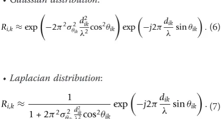
If we consider the diffuse component and we assume a small AS value (s_θ<ssmall), then the correlation coef-ficientRi, k would be [14,18]

•Gaussian distribution:

Ri,k≈exp

−2π2σ_θ2_ikd 2 ik

λ2cos 2_θ

ik

exp

−j2πdik

λ sinθik

.(6)

•Laplacian distribution:

Ri,k≈

1

1 + 2π2_σ2

θik d2

ik

λ2cos2θik

exp

−j2πdik

λ sinθik

.₍₇₎

In this study, we are interested in estimating the mean AoA and the AS. In other terms, we determine the mean and the standard deviation of the angular ditribution of the received signal. The proposed algo-rithm is valid for non linear antenna arrays. Hence, each antenna branch represents different mean AoA and AS estimation values. That is why the parameters in question are function of the indexes i and k which refer to the associated antenna pair (i, k), as shown in Figure 2. As noticed, the two pairs (i, k) and (k, l) represent different mean AoA and AS values,(θik, σθik) and(θkl, σθkl). Each couple is estimated using the cor-relation coefficients, Ri, k and Rk, l, respectively. This model formulation with global parameters can be advantageous in a parameter estimation framework, when evaluating the Cramér Rao bound (CRB), for instance. In the following, we develop a new mean AoA and an AS estimator based on the correlation coefficient defined in (3).

III. New estimator with angular distribution selection

The idea is to find a simple relationship between the mean AoA and AS, and the Rician correlation coeffi-cient. Since the expression of the Rician correlation coefficient RTikis complex, our approach is to estimate the LOS component first. Then, the diffused compo-nent Rik is deduced, and the AS is extracted from LUTs. For each angular distribution type, a LUT is built off-line using the expression (5) for the NLOS component of the correlation coefficient. Indeed, for all possible values of the mean AoA and AS, the corre-lation coefficient of the diffuse component is computed using a numerical method (5). In our simulations, we varied the mean AoA from 0 to 90 degrees with a step of 0.1 degree. The AS is varied from 0 to 100 degrees with a step of 0.025 for small ASs (s_θ <6 degrees) and a step of 0.1 degree for higher ones. One can argue that the building of the LUT using the considered steps requires a lot of time and an accurate resolution of the integral in (5). However, the LUT is computed once for all off-line and would not affect the real-world execution time of the new algorithm. Besides larger steps would affect the accuracy of the new esti-mator. The LUT expresses the desired parameterbas a function of the magnitude and phase of the diffuse component Rik. As defined in (4), the LOS component depends only on the Rician K-factor and the AoA of the LOS. In this study, we consider uniform clusters. Hence, the AoA of the LOS coincides with the mean AoA. If we assume small AS values and consider the diffuse component of the correlation coefficient (6) associated to the Gaussian distribution, then the rela-tionship in (4) becomes

RTi,k = 1

K+ 1exp

−2π2σ_θ2ik

d2 ik

λ2cos 2

(θik)

exp

−j2πdik

λ sin(θik)

+ K

K+ 1exp

j2π(d0i

λ sin(θ0i)− d0k

λ sin(θ0k))

.

(8)

Considering only antenna-element pairs including the antenna-element reference “0″, both terms of the

correlation coefficientRT0,kadmit the same argument:

RT0,k=

1

K+ 1exp

−2π2_σ2 θ0k

d2 0k

λ2cos

2_(θ0k)

+ K

K+ 1

exp

−j2πd0k

λsin(θ0k)

. (9)

Hence, the mean AoA is estimated by using the phase of the correlation coefficient associated to the antenna pairs (0,k). By analogy, the same expression is obtained for the Laplacian distribution:

ˆ

θ0k= arcsin

− RˆT0,k

2πd0k λ

, (10)

where∠ symbolizes the phase operator and the sub-script“0″refers to the antenna-element reference and the distance separating the antenna-element pair (0,k) is such that d0k≈ λ₂. As one can notice, we use only the antenna-elements pair (0, k) to estimate the AoA LOS. Otherwise, the correlation coefficient of the dif-fuse component,Ri, k, and the correlation coefficient of the LOS component would admit different arguments (see (8)). The final mean AoA estimate, _θˆ_m, is the mean of _θˆ_0k over all antenna-elements pairs {(0, k)} spaced by λ₂. Indeed, the antenna pairs spaced by d0k ≫ l give high estimation error since the correlation coefficient does not contain enough information, i.e., RT0,kis close to zero. It is understood that (10) is valid for antenna configurations having at least two antenna-element spaced by λ₂. In most references, ULAs spaced by λ₂are considered. Hence, our condi-tion enlarges the set of possible antenna arrays that can be used. One can argue that 10 this solution does not take into account the left-right ambiguity. Indeed for linear arrays (antenna-element pairs in our case), it is not obvious to determine whether the incident signal is coming from the left side or the right one of the array [19,20]. To avoid this ambiguity, we divide the cell into three or more sectors and the mean AoA esti-mation is achieved in each sector. In the remainder of this article, (10) is used for antenna-element pairs for which the left-right ambiguity does not arise. In other words, we imply that the arrays are constructed in a way that prevents this ambiguity by considering the cell division approach or other methods as in [19]. Indeed, this condition limits the subset of antenna structures that can be used for the mean AoA estima-tion, but still allows some flexibility in the design of antenna arrays. Without loss of generality, we consider the antenna configurations illustrated in Figure 1. All structures are supposed to be constructed in a way that prevents the left-right ambiguity. For these sym-metrical structures, after a simple mathematical manip-ulationc, it is observed that (10) is also true for

correlation coefficients RˆTi,k associated with antenna-element pairs (i, k) spaced bydik≈ λ₂, i.e., the antenna pairs (0,1) and (1,2) of all structures presented in Fig-ure 1. The angles must have the same reference which in this case the normal to the antenna structure, and the clockwise sense is the positive one. The AS estima-tion is not affected by the choice of the angles mea-surement reference. Indeed, it measures the angular distribution spreading around the mean AoA. One can argue that relation (10) is only valid for small AS values assumption. However, we empirically find that the mean AoA estimate using (10) is still accurate for high AS values.

For the Rician factor, many K-factor estimators have been developed. In [21], the Kolmogorov-Smirnov statis-tic is used first to test the envelope of the fading signal for Rician statistics and then to estimate theK-factor. In [22], theK-factor estimator is based on statistics of the instantaneous frequency (IF) of the received signal at the mobile station. In [23], ML estimators that only use samples of both the fading envelope and the fading phase are derived. In [24] and [25], a general class of moment-based estimators which uses the signal envel-ope is proposed. AK-factor estimator that relies on the in-phase and quadrature phase components of the received signal is also introduced in [24].

We choose to consider the closed-form estimator pre-sented in [24], which is easily implemented and quite accurate. This estimator uses the second-order and fourth-order moments (μ2 andμ4) of the received signal to estimate theK-factor (shown here for the estimate on theith antenna):

Ki=

−2μ2

i;2+μi;4−μi;2

2μ2 i;2−μi;4 μ2

i;2−μi;4

. (11)

The final K-factor estimate is the mean ofKˆiover all antenna-elementsi.

In [26], the expressions for the second-order and fourth-order moments at antenna-elementiare:

μi;2=+N0andμi;4=ki;a+ 4N0+ki;ωN20, (12)

where Ωand N0 are, respectively, the signal and the noise powers; and ki;a and ki;ω are, respectively, the

Rician and noise kurtosis. In our article, we consider an additive white Gaussian noise (AWGN), i.e., ki;ω= 2,

[26]. As in [14], we consider an estimated _SNRˆ to reduce the noise bias. The expressions of the second-order and fourth-second-order moments become

ˆ μi;2=

1 N

N−1

n=0

|xi(n)|2

SNRˆ SNRˆ + 1

andμˆi;4=

1 N

N−1 n=0

|xi(n)|4 ki;aSˆ NRˆ 2

ˆ

In the literature, the value ofki;ais computed by using the RicianK-factor which is unknown at this stage [27]. In our procedure, the Rician kurtosiskˆi;ais obtained by analyzing the term

N−1 n=0 |xi(n)|4

(Nn=0−1|xi(n)|2)

2 and is computed as

fol-lows:

ˆ

ki;a=

(SNRˆ + 1)2

N−1

n=0 |xi(n)|4 (N_n=0−1|xi(n)|2)

2 −4SNRˆ −2

SNRˆ 2 .

(14)

Several SNR estimators can be considered, such as in [28,29] or [30]. In this article, we do not consider a spe-cific SNR estimator, to avoid restricting our algorithm to a particular SNR estimator results. Instead, we con-sider an estimated SNR expressed indB,(SNRˆ dB). The latter is characterized by an estimation error modeled as a zero-mean normally distributed random variable with variance σ2

ε, i.e., SNRˆ dB=SNRdB+ε, where

ε∼N(0, σ_ε2). As shown in [28], the studied estimators offer low estimation errors, especially for long observa-tion windows. For the SNR range considered in our simulations, the variance of the estimation error is around 10-1. Hence, we choose extreme cases where

σ2

ε = 0or 1 (i.e., optimistic and pessimistic bounds).

With AWGN bias reduction, the expression for the estimated Rician correlation coefficient (fori≠k) is

ˆ

RTi,k=

N−1

n=0 xi(n)xHk(n)

N−1

n=0 |xi(n)|2Nn=0−1|xk(n)|2

SNRˆ SNRˆ +1

. ₍₁₅₎

Once the AoA of the LOS and the RicianK-factor are estimated, the estimated NLOS componentRˆikis then deduced:

ˆ

Ri,k= (Kˆ+ 1)

ˆ

RTi,k−

ˆ

K

ˆ

K+ 1exp(j2πmˆik)

, (16)

where mˆik= d_λ0i sin(θˆ0i)−d_λ0ksin(θˆ0k). When the antenna-elements separationd0k> λ₂, we takeθˆok=θˆm. Note that all angle measurements must have a common reference. The AS is extracted from the LUT associated to the considered angular distribution type. Using linear interpolation, we determine which AS value corresponds to the magnitude and phase of the estimated correlation coefficient Rˆi,k. In this article, we treat the case when the a priori knowledge of the angular distribution is assumed. In this case, arbitrary arrays can be used including ULAs. We also propose a new method to determine the angular distribution of the received signal when it is unknown. In this case, a nonlinear array is required. In fact, we select the angular distribution type that fits the array geometry from a set of possible

candidates. Different mean AoAs and ASs are obtained for the different antenna branches which is not the case for linear structures. Then, the selected angular distribu-tion is the one associated with the minimum of the esti-mates’ standard deviations. The level of accuracy for small AS values is taken into account as well. Indeed, (6) and (7) are computed assuming small AS values. As a result, we must first rank the AS. Then, if the latter is low, we can apply (6) or (7). In fact, the LUT approach shows low accuracy for small ASs. That is why we pre-sent here four variants of the new AS estimator depend-ing on the knowledge of the angular distribution and the desired accuracy of the AS estimation.

A. Known angular distribution type and low AS estimation accuracy for small AS values

Let us first study a simple case. Consider a pair of antenna-elements (0, 1) spaced byd01≈ λ₂. We first

esti-mate the LOS component, i.e., the K-factor and the mean AoA (using (10)). Owing to the estimated NLOS component Rˆ0,1, we obtain the AS estimate,σ˜₀₁(c)from

the LUT associated with the considered distribution type,g. The procedure is summarized as follows:

ˆ

K= −2μˆ22+μˆ4− ˆμ2

√

2μ2 2−μ4

ˆ

μ2

2− ˆμ4 ,

ˆ

θm= arcsin

− RˆT0,1

2πd0,1

λ

,

ˆ

R0,1= (Kˆ + 1)

ˆ

RT0,1−

ˆ K ˆ K+1e

j2πmˆ01

,

˜

σ(c) 01 =LUTγ

| ˆR0,1|, Rˆ0,1

.

(17)

where μˆ2;iand μˆ4;i are the estimated second-order and fourth-order moments, respectively. When the antenna array is composed of more than two elements, the procedure is applied to each pair. The final AS estimate σˆR is the mean of all σ˜_ik(c)divided by (K+1). The division by (K+1) is employed to recover the NLOS AS from the one associated to the Rician chan-nel. When a uniform linear array (ULA) is used, the estimation error can be reduced even more by aver-aging the correlation coefficients over all antenna pairs spaced by the same distance, before using the LUT, instead of averaging the individual AS estimates over all antenna pairs.

B. Unknown angular distribution type and low AS estimation accuracy for small AS values

select the distribution type from a set of possible candi-dates. The idea is to seek the distribution type that best fits the geometry of the array. A nonlinear array structure such as the one illustrated in Figure 1b, where the closest antenna-elements are spaced by≈λ₂or less, has to be considered. The anglevalue is not static and can be modified to fit the base station construction constraints. As in the previous case, we estimate the LOS component. Then, for each antenna pair (spaced byd≈ λ₂) and each distribution typeg, the mean AoA_θˆ_ik(γ)and AS_σ˜ik(c)(γ) are extracted fromLUTg. In this case, the estimated

mean AoA is actually the sum of the received signal mean AoA,θik, and the angle of nonlinearity ±. Hence, to recover the desired mean AoA, we substract the angle ±(see the algorithm below). The selected distri-bution type(γˆ)is the one associated to the minimum of

the sum of the standard deviations

σaoa(γ) = std{ ˆθ01(γ),θˆ12(γ)}andσas(γ) = std{ ˜σ01(c)(γ),σ˜ (c) 12(γ)}

of the estimated parameters:

σaoa(γ) = std

ˆ

θik(γ); (i, k) such thatdik≈ λ 2

, (18)

σas(γ) = std

˜ σ(c)

ik (γ); (i, k) such thatdik≈ λ 2

, (19)

ˆ

γ = min

γ {σas(γ) +σaoa(γ)}. (20)

The chosen criterion is motivated by the nonlinearity of the array. For instance, using the configuration illu-strated in Figure 2, the mean AoA impinging at the pair (i, k),θik-, must be close to the one associated to the branch (k, l), θkl + . Indeed, we assumed the same parameter values at the different array elements. How-ever, by considering the wrong distribution type, the obtained mean AoAs would be different and as a result show high standard deviation. The same reasoning is adopted for the ASs estimates (19). One can argue that the mean of the AS estimates could be used instead of the standard deviation in (19). Actually, the mean of the obtained estimates would not give us any information about the angular distribution of the received signal. For instance, for the array structure illustrated in Figure 2b, we obtain two AS estimates associated to the Gaussian and Laplacian distributions. In this case, we cannot select the right angular distribution. This is why we con-sider the standard deviation of the AS estimates.

For the mean AoA estimation, we no longer require antenna pairs including the antenna reference“0”, but instead each pair (i, k) separated by l/2. Indeed, once the LOS component is determined and the diffuse com-ponent is deduced, we use (6) or (7) to estimate the mean AoA. The considered expressions are not

restricted to antenna pairs (0,i) but to all antenna-ele-ments (i, k).

Note that the procedure above estimates the mean AoA twice. In (10), the resulted mean AoA is used to compute the LOS component. Mean AoAs are then extracted from a LUT using the diffuse component of the Rician correlation coefficient. These estimates are employed to select the angular distribution by comparing their standard deviations (18). One can argue that the standard deviations of the AS could be used instead of estimating the mean AoA twice. However, when the AS is small, the angular distribution is close to an impulse function for both distribution types. In fact, the mean AoA standard deviations bear more information concern-ing the distribution type. In this case, the distribution type selection using the criterion (20) is no longer due to its high error rate. To overcome this limitation, we look for weights that express the importance of one parameter compared to the other, i.e., weights that ensure better selection. After running exhaustive simulations, results show that when the AS is small (s<sthreshold), only the standard deviation of the mean AoA estimates (18) must be considered. Even when the AS is high, the two stan-dard deviations,saoaandsas, should not be considered with the same importance. Indeed, a larger weight should be affected to the information provided by the standard deviation of the mean AoA estimates. Hence, the optimal weights were empirically set equal to

ωas=χ_[maxγ(σ˜(c)_(γ))>σ

threshold], (21)

ωaoa=χ_[maxγ(σ˜(c)_(γ))≤σ threshold]+

3

2χ[maxγ(σ˜(c)_(γ))>σ

threshold],(22)

whereσ˜(c)_{(γ)is the mean of the estimated AS}

asso-ciated with the gth angular distribution and c is the function defined by

χ[A]=

1 if the eventAis true,

0 otherwise. (23)

sthresholdwas set empirically to 6°. In fact, this value depends also on the distribution type. In other words,

σγ1

threshold=σ

γ2

threshold. In this study, we consider the same

sthreshold for both considered distribution types, to sim-plify implementation. Still, for more accuracy, one could use different values for each distribution type. The selected angular distribution type is then the one asso-ciated with the minimum of the weighted sum, so that, instead of (20), the following is used:

ˆ

γ = min

γ {ωas(γ)σas(γ) +ωaoa(γ)σaoa(γ)}. (24)

selected angular distribution. The overall procedure is as follows:

ˆ

K= mean

−2μˆ2 i;2+μˆi;4− ˆμi;2

√ 2μˆ2

i;2− ˆμi;4

ˆ μ2

i;2− ˆμi,4

ˆ

θik= arcsin

− _Rˆ_ij

2πdik_k

fordik≈ λ₂

ˆ

θm= mean

ˆ

θ01+ϕ;θˆ12−ϕ

ˆ

R= (Kˆ + 1)RˆT−_KˆKˆ₊₁ej2πM

ˆ

R(_i,c_k)=Rˆi,kχ[dik≈ λ₂]

= number of considered angular distributions Forγ= 1 to

˜ σ(c)

ik (γ),θˆik(γ)

=LUTγ(| ˆR_i(_,c_k)|, θ_Rˆ(c) i,k)

σaoa(γ) = std({ ˆθik(γ)/dik≈ λ₂})

σas(γ) = std ({ ˜σik(c)(γ)/dik≈λ2}) ˜

σ(c)_{(γ) = mean ({ ˜σ}(c) ik (γ)})

ˆ

θm(γ) = mean ({ ˆθik(γ)}) End

(25)

ωas=χ_[maxγ(σ˜(c)_(γ))≥σ threshold] ωaoa=χ[maxγ(σ˜(c)_{(γ))<σthreshold]}+. . .

3

2χ[max_γ(σ˜(c)_{(γ))≥σthreshold]}

ˆ

γ = min

γ (ωasσaoa(γ) +ωaoaσaoa(γ))

ˆ

θm=θˆm(γˆ)

ˆ

σθ=σ˜(c)(γˆ)

ˆ

σR=_Kσˆ₊₁θ

(26)

C. Known angular distribution type and high AS estimation accuracy for small AS values

With small AS values, closed forms can be deduced from (6) and (7):

•Gaussian distribution:

θik= arcsin

− Ri,k 2πdik

λ

wheredik≈ λ

2, (27)

σik=

−2 ln|Ri,k| 2πdik

λ cos(θik)

. (28)

• Laplacian distribution: The mean AoA has the

same expression as in (27), and

σik=

2 |Ri,k|−2 2πdik

2 cos(θik)

. (29)

The analysis of (28) and (29) shows that, when the correlation coefficient amplitude is close tooneor zero, the AS estimation error is higher. Indeed, in this case, the estimation error of the correlation coefficient has an important impact on the AS estimation. The solution to their problem is to consider distant antenna-elements spaced by d≫ l. Indeed, in this case, the correlation coefficient amplitude is reduced. To avoid correlation coefficients with a magnitude too close tozero, we set empirically (i.e., by running several simulations) a lower limit of 0.05 to decrease the estimation error. In other terms, we exploit only distant antenna-element pairs for which the correlation coefficient magnitude is higher than 0.05.

To illustrate the overall AS estimation process, we consider the array configuration illustrated in Figure 1c. In this section, we consider the a priori knowledge of the angular distribution type. The procedure is then as follows. After estimating the LOS component and dedu-cing the diffuse one, we consider first the closest pair of antenna-elements (Ant.0-Ant.1). From the 2-DLUT, we estimate the AS_σ˜01(c). If the obtained preliminary AS is larger than ssmall, (28) and (29) are not to be consid-ered, and the procedure is terminated. Otherwise, we use the distant elements (Ant.1-Ant.2) and the closed-forms provided by (28) and (29) to estimate the AS_σ˜12(d). The overall AS estimation procedure is as follows:

ˆ

K= mean

−2μˆ2 i;2+μˆi;4− ˆμi;2

√

2μˆ2 i;2− ˆμi;4

ˆ μ2

i;2− ˆμi;4

ˆ

R= (Kˆ + 1)

ˆ

RT−_KˆKˆ₊₁ej2πM

Ifσ˜(c)(k)ˆ < σsmalland| ˆR1,2| >0.05

ˆ

σθ=g(θmˆ , | ˆR1,2|)

The functiongrefers to (28) or (29) Else

ˆ σθ=σ˜01(c)

End

ˆ σR= σˆθ

ˆ

K+1

(30)

D. Unknown angular distribution type and high AS estimation accuracy for small AS, values

and the existence of distant antenna-elements for a high estimation accuracy in the case of small AS. The butter-fly configuration presented in Figure 1d is then consid-ered as an example. Other structures satisfying the conditions mentioned above could be used.

Once the LOS component is estimated and the diffuse one is deduced, as in the previous cases, we consider first the closest antenna-elements (spaced by ~λ₂). For each angular distributiongand antenna pair (i, k) spaced by aboutλ₂, we extract the associated mean AoA_θˆik(γ)and AS_σ˜ik(c)(γ)fromLUTg. Then, we compute the associated

standard deviations,saoa(g) andsas(g). The selected distri-bution typeγˆis the one associated to the minimum of the weighted sum [see (24)]. If the preliminary AS

˜

σ(c)_{(γˆ) = mean (σ˜}(c)

ik (γˆ))is larger thanssmall, then closed forms of (28) and (29) are not to be considered, and the procedure is terminated. Otherwise, for accurate AS esti-mation, we consider the distant antenna-elements (d≫l) with a correlation coefficient amplitude higher than 0.05. The latter is chosen empirically after several simulations. A correlation coefficient with a lower module would not have enough information to allow the AS estimation. Then, for each considered pair and each distribution type, we estimate the AS_σ˜(d)

ik (γ)using (28) and (29). During simulations, we noticed that the standard deviations of the AS estimates obtained using distant antenna-elements offer lower error probability of distribution type selection. A second angular distribution selection is therefore con-sidered, for which at least two AS estimates(σ˜_ik(d)(γ))are needed. If the number of correlation coefficients with a module higher than 0.05 is inferior to 2, then we cannot compute the standard deviation of one AS estimate. In this case, the procedure is terminated, and the final AS is the preliminary AS associated with the selected distribu-tion typeγˆ. Otherwise, we compute the standard devia-tions of the estimated AS obtained using the distant antenna-elements(σ˜_ik(d)(γ)):

σas(γ) = std

˜

σ(d)

ik (γ); (i,k) such thatdik λand| ˆRik|>0.05

. ₍₃₁₎

The selected angular distribution,γˆf, is the one asso-ciated with the minimum of the sum (24) (using the standard deviations of the AS estimates of distant ele-ments). The final mean AoA estimate,_θˆ_m, is then the mean AoA associated with the selected distribution type,γˆf. The final AS estimate is the mean of the AS estimates over distant antenna pairs associated withγˆf, i. e., the estimated AS is

ˆ

σθ= mean

˜

σ(d)

ik (γˆf)

. (32)

The overall AS estimation procedure is summarized as follows:

ˆ

K= mean

−2μˆ2

i;2+μˆi;4− ˆμi;2√2μˆ2i;2− ˆμi;4

ˆ μ2

i;2− ˆμi;4

ˆ

θik= arcsin

− r_ˆik

2πdik_λ

fordik≈λ2

ˆ

θm= meanθˆ01+ϕ;θˆ12−ϕ

ˆ

R= (Kˆ + 1)RˆT−_KˆKˆ₊₁ej2πM

ˆ

R_i(_,c_k)=Rˆi,kχ_dik≈λ

2

ˆ

R(_i,d_k)=Rˆi,kχ[dik λ]

= number of considered angular distributions Forγ = 1 to

˜ σ(c)

ik (γ),θikˆ (γ)

=LUTγ(| ˆR(_ikc)|, θ_Rˆ(c) i,k) σaoa(γ) = std ({ ˆθik(γ)/dik≈λ2}) σ2

as(γ) = std ({ ˜σ (c)

ik (γ)/dik≈λ2})

˜

σ(c)_{(γ) = mean ({ ˜σ}(c) ik (γ)}) ˆ

θm(γ) = mean ({ ˆθik(γ)}) End

ωas=χ_[maxγ(σ˜(c)_(γ))≥σ threshold] ωaoa=χ_[maxγ(σ˜(c)_(γ))<σ

threshold]+. . . 3

2χ[maxγ(σ˜(c)_(γ))≥σ threshold] ˆ

γ = minγ(ωasσaoa(γ) +ωaoaσaoa(γ)) cardE= cardinal{(i, k)/| ˆR_i(_,d_k)|>0.05}

Ifσ˜(c)(γˆ)> σsmall

ˆ

σθ=σ˜(c)(γˆ)

ˆ

θm=θmˆ (γˆ) Else IfcardE<2

ˆ

σθ=σ˜(c)(γˆ)

ˆ

θm=θmˆ (γˆ) Else

Forγ = 1 to

˜ σ(d)

ik (γ) =g(θˆ(γ),| ˆR (d)

i,k|>0.05)

The functiongrefers to (28) or (29)

σas(γ) = std({ ˜σ_ik(d)(γ)}/dik λ)

End

ˆ

γf=minγ(ωasσaoa(γ) +ωaoaσaoa(γ))

θm=θmˆ (γfˆ)

ˆ

σθ= mean({ ˜σij(d)(γfˆ)})

End End

ˆ σR= σˆθ

ˆ

K+1

IV. Other as estimation methods selected for performance comparison

In this article, we compare the new AS estimator to other low-complexity algorithms. As mentioned before, there exist more robust estimators [2] and [10], but our pur-pose is to evaluate low complexity estimators. Spread Root-MUSIC is therefore the appropriate candidate for performance evaluation and comparisons. We also com-pare the new AS estimator with the two-stage approach [13] which is based on the Spread Root-MUSIC principle.

A. Extended spread Root-MUSIC to 2-D arbitrary arrays

The principle is to localize two rays symmetrically posi-tioned around the nominal AoA. Then, the AS is esti-mated by using a LUT symbolized by the function

Λ(s_ω) computed by considering a mean AoAθm= 0. In [14], Spread Root-MUSIC for a ULA with inter-ele-ment spacing d= λ₂, in the presence of a LOS, is pre-sented as follows:

{ˆν1,νˆ2}= Root−MUSIC(Rˆc, nb.sources= 2), (34)

ˆ

ω= νˆ1+νˆ2

2 , (35)

ˆ

θm= arcsin

ˆ

ω

2πd_λ

, (36)

ˆ

σR=

−1

K

|ˆν1−ˆν2|

2

2πd_λcosθˆm

, (37)

whereRˆci,k =

1

N

N−1

n=0 xi(n)xHk(n)is the estimated cov-ariance matrix, andνˆi= 2πd_λsin(θˆi)is the spatial fre-quency, θmis the mean AoA,σˆRis the AS of the Rician fading channel, andΛK(sω) is the function defined by

{K(σω), −K(σω)}= Root−MUSIC(Rc(θm= 0,K), 2).(38)

where σ_ω= |ν1−ν2|

2 . Note that the function ΛK(sω)

depends on the RicianK-factor. To reduce the poten-tially large number of LUTs, we propose to consider the estimation and the extraction of the LOS component for Spread Root-MUSIC, as does our new estimator. In other words, we consider only the NLOS component instead of considering the total estimated covariance matrixRˆc. In this case, one functionΛ(sω), with K= 0, is considered. The relationship in (37) becomes

ˆ

σR=

−1|ˆν1−ˆν2|

2

2πd_λ(K+ 1) cosθˆm

. (39)

As presented in [5], Spread Root-MUSIC estimates the AS and mean AoA for ULAs. In this article, we adapt Spread Root-MUSIC to the butterfly configuration to be able to evaluate the performance of the new method. In [31], those authors propose an extension of Root-MUSIC to 2-D arbitrary arrays. Since Root-Root-MUSIC exploits the Vandermonde structure of the steering vec-tor of ULAs, the idea is to rewrite the steering vecvec-tora

of nonlinear arrays as the product of a Vandermonde structured vector d and a matrixGcharacterizing the antenna configuration (manifold separation) [31]:

a(θ)≈Gd(θ). (40)

The matrix G can be determined using the least square (LS) method as follows:

G=ADH(DDH)−1. (41)

Once the characteristic matrix is built, the MUSIC-spectrum is then rewritten as a function of the new steering vector:

SMUSIC(θ) = (dH(θ)GHEnEHnGd(θ))−1. (42)

where En is the matrix containing the eigenvectors associated to the noise subspace. As is noticed, the new noise subspace is no longer defined by the eigenvectors of the covariance matrix associated to the smallest eigenvalues, but by the product of the characteristic matrix and the eigenvectorsEn. The estimated AoAs are then the arguments of the complex roots of the obtained pseudospectrum. One drawback of the extended Root-MUSIC algorithm is the heavy computa-tions of the pseudo-spectrum. For instance, in our case, to ensure the required accuracy, the dimension of the characteristic matrix is set to (360 × 151), thereby increasing the algorithm’s complexity significantly.

The modified Root-MUSIC still fulfills the properties of a consistent estimator. Hence, we can apply the Spread Falgorithm described in [5]. Our new extended spread Root-MUSIC (ESRM) algorithm can be applied as follows:

ˆ θ1,θˆ2

= Root−MUSIC−Butterfly (Rˆc,nb.sources= 2),(43)

ˆ

θm=

ˆ

θ1+θˆ2

2 , (44)

ˆ

σR=

−1| ˆθ1− ˆθ2|

2

(K+ 1) cosθˆm

. (45)

observed in the Root-MUSIC approach. The extended version of Spread Root-MUSIC computes directly the physical angles _θˆi, i= 1, 2 instead of the spatial frequenciesv_ˆi, i= 1, 2, (34). The mean AoA _θˆ_mis then the mean of the estimated AoAs.

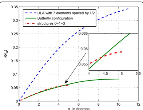
In Figure 3, we compare the functionsΛ(s_ω) obtained for both ULA and butterfly configurations (see Figure 1d). Since our nonlinear structure presents distant antenna-elements spaced by 3l, we consider a ULA with seven elements spaced byλ₂. Note that while a ULA configuration can estimate AS values higher than 10°, the functions Λ(sω) of the butterfly and (0-1-3)

struc-tures show lower limits.

B. Angular distribution selection using ESRM

As mentioned before, the new AS estimator selects the angular distribution according to the standard deviations of the mean AoA and AS estimates. In this article, we adopt the same approach for the ESRM. As in our method, we need two symmetric structures with at least a 3D correlation matrix. Indeed, ESRM will require two dimensions for the signal subspace and another one for the noise subspace. In this case, one can consider the following antenna-elements combinations (see Figure 1d: (Ant.0-1-3) and (Ant.2-1-4). To build the function

Λ(sω), Root-MUSIC requires symmetric structures. In

our case, the considered array structures give the follow-ing results:

{1(σ),2(σ)}= Root−MUSIC(Rc(θm= 0,K= 0), 2), (46)

whereRcis the covariance matrix. We then consider the functionΛ(sω) define by

(σω) = |1(σω)|+|2((σω))|

2 . (47)

The resulting function keeps the same properties as for symmetric arrays.

Once we build the function Λ(s_ω), we apply the Spread Falgorithm [5] to estimate the AS. At this step, for each angular distribution type (g), two AS estimates are obtained. The firs one, s013(g), is associated to the structure Ant.(0-1-3) and the second, s214(g), is asso-ciated to the structure Ant.(2-1-4), see Figure 1d. The selected angular distribution type(γˆ)is the one asso-ciated with the minimum of the standard deviations of the AS estimates:

ˆ

γ = min

γ (std(σ013(γ), σ214(γ))). (48)

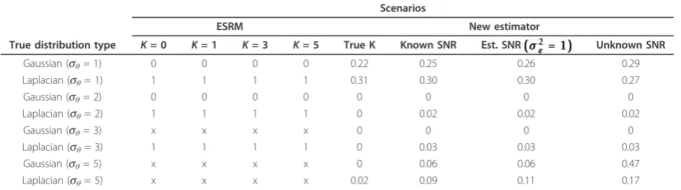
Simulations show that the angular distribution selec-tion using ESRM is irrelevant. Whether the distribuselec-tion type is Gaussian or Laplacian, the same mean AoA is observed. Indeed, (43) does not require the knowledge of the angular distribution type. That is why the stan-dard deviation of the mean AoA estimates is not used in (48). Moreover, as shown in Figure 3, ESRM cannot estimate an AS higher than 4° using the structures (0-1-3) and (2-1-4). Using the same AS value in both struc-tures, the angular distribution selection cannot be achieved considering the standard deviation of AS esti-mates. These cases are marked “x” in Table 1. This is why the a priori knowledge of the angular distribution type is required for ESRM.

C. The two-stage approach

In [13], a new two-stage approach similar to Spread Root-MUSIC was presented. The estimation of the mean AoA and the AS of the scattered source is trans-formed there into the localization of two closely spaced point sources. The new approach approximates the function Λ(s_ω) by a linear function. Indeed for a ULA with M antenna-elements spaced byd= λ₂, Λ(sω)≈ sω.

As noticed, the function Λ(s_ω) no longer depends on the angular distribution type. In other terms, the selec-tion of the distribuselec-tion type is not required for the two-stage approach. The algorithm is as follows:

ˆ dm= 1

M−m M−m

l=1 Rˆcl+m,l ˆ

ω(1)_{= (d}ˆ 1)

ˆ

θ= arcsin

ˆ

ω(1)

2πd

ˆ

ω(M−1)₌ (dˆM−1)

M−1 ˆ

δ(M−1)

ω =

1

M−1arccos

RdˆM−1

ˆ

d0 e

−j(M−1)ωˆ(M−1)

ˆ

σθ= δˆ

(M−1) ω

2πdcos(θˆ)

(49)

0 2 4 6 8 10 12

0 0.05 0.1 0.15 0.2 0.25 0.3 0.35

σ_θ in degrees

Λ

(

σθ

)

ULA with 7 elements spaced by λ/2 Butterfly configuration

structures 0í1í3

4 4.5 5 5.5

0.055 0.06 0.065

where ∠(.) andR(.)represent operators that extract, respectively, the angle and the real parts. As other esti-mators, the approach described in [13] considers only LOS-free scenarios. In this article, we consider, as for ESRM and the new estimator, the NLOS component of the covariance matrix. The method exploits the Toeplitz structure of the covariance matrix by averaging the coef-ficient of the mth subdiagonals of Rˆc. It was shown in [13] that the covariance coefficients on the first subdia-gonals give better mean AoA estimates. Simulations in [13] showed also that antenna- elements spaced by 2.5l offer better AS estimation. For the butterfly configura-tion, the algorithm described above can be applied by considering antenna pairs. In other terms, the antenna-elements spaced by d= λ₂ are utilized to estimate the mean AoA and the distant ones are considered for the AS estimates. In this article, we select the antenna pairs spaced by 3l, the closest distance to the one used in [13]. Indeed, the pairs (ant.1-ant.3) and (ant.1-ant.4) can be modeled by a ULA composed by six antenna-ele-ments. In this case, the algorithm of the two-stage approach is applied withm= 5.

V. Simulation results

We illustrate the performance of the new AS estimator by means of Monte-Carlo simulations. We assume here that the channel coefficients are obtained through an appropriate channel estimation algorithm, and that the resulting time-varying channel coefficient estimates can be adequately modeled by the sum of the true time-varying channel coefficients with an AWGN component. The accuracy of the channel estimation procedure is then controlled by the variance of the AWGN compo-nent. In our simulations, for the diffuse component, we used a non-selective frequency (f at) Rayleigh channel. We considered the Rayleigh channel simulator described in [32]. The azimuth AS distribution for the incoming multipath signals are of Gaussian or Laplacian type. The carrier frequency was set to 1.9 GHz, which results in a

wavelength lof 15.79 cm. The mobile speed was set to 80 Km/h (22.2 m/s), which results in a Doppler fre-quency FDof 140.74 Hz. The sampling interval was set toTs= ₁₅₀₀1 ms. The SNR of the estimated channel coef-ficients is 15 dB.

First, we study the new estimator performance when the angular distribution is known. In this case, we con-sider a ULA with five antenna-elements spaced by a half wavelength. We compare the algorithm described in III. C. with the weighted least square (WLS) method and the stochastic CRB developed in [10]. In this article, we consider the unknown parameter vector defined as

η= [Sσ2

nσθθm], whereSandσn2are the transmitted signal and noise powers. In [10], the varianceσ2

θ is considered

instead of s_θ. Thereby, we recompute the CRB using (13) of [10]. The normalized mean square error (NRMSE) is used to evaluate both estimators:

NRMSE(σ_θ) =

1

N

N

n=1(σˆθ−σθ) 2

σθ .

(50)

As shown in Figure 4, for mean AoA estimation the new estimator presents lower NRMSE and is the closest one to the CRB. For the AS estimation, the new estima-tor and the WLS method present close NRMSE (see Figure 5), for different computational complexities. For instance, the Gauss-Newton method used in the WLS technique converges in around 600 iterations, which increases significantly its computational complexity. One can also notice that the SNR estimation error does not affect the mean AoA and AS estimation. Indeed, whether the SNR is assumed known or with a Gaussian estimation error with variance σ2

ω = 1, both estimators

show the same results.

Second, we study the angular distribution selection and its impact on the new estimator. To this purpose, we consider the butterfly configuration withj = 10°,

d01=d12= λ₂, and d13 = d14 = 3l. Since it does not

Table 1 Error probability of angular distribution selection

Scenarios

ESRM New estimator

True distribution type K= 0 K= 1 K= 3 K= 5 True K Known SNR Est. SNR(σ2

ε =1) Unknown SNR

Gaussian (sθ= 1) 0 0 0 0 0.22 0.25 0.26 0.29

Laplacian (sθ= 1) 1 1 1 1 0.31 0.30 0.30 0.27

Gaussian (sθ= 2) 0 0 0 0 0 0 0 0

Laplacian (sθ= 2) 1 1 1 1 0 0.02 0.02 0.02

Gaussian (sθ= 3) x x x x 0 0 0 0

Laplacian (sθ= 3) 1 1 1 1 0 0.03 0.03 0.03

Gaussian (sθ= 5) x x x x 0 0.06 0.06 0.47

Laplacian (sθ= 5) x x x x 0.02 0.09 0.11 0.17

allow the proper selection of the angular distribution type, the a priori knowledge of the angular distribution type is assumed for ESRM. To study the effect of theK -factor estimation error and the variance of the estimated

σ2

ε,σε2, on AS estimation, we consider several scenarios.

In the first one, we assume the a priori knowledge of theK-factor, i.e., we use the true value of the K-factor to estimate the diffuse component. In the second case, we consider the true value of the SNR. In the last two cases, an estimated_SNRˆ with varianceσ2

ε = 1is used.

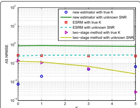
As shown in Figure 6, the new estimator shows lower NRMSE for the mean AoA estimation. In Figure 7, the AS estimation with the variation of theK-factor value is studied. As noticed, the new estimator presents high NRMSE when the SNR is assumed unknown. As

mentioned before, this is due to the important estima-tion error exhibited by the K-factor estimator (11). Indeed, If we consider the true value of theK-factor, the new estimator achieves more accurate results. The ESRM and the two-stage approach also show lower NRMSE when the true K-factor is assumed, especially when its value is high.

One can argue that the new estimator fails in the case of unknown SNR. Note that while ESRM requires the eigen-decomposition of the covariance matrix and find-ing the roots of a polynomial, our method uses only LUTs, simple closed forms, and some logical operations. Indeed, the Spread Root-MUSIC shows high complexity around M3_{log(M) +M}2_(N

a+T) +N2aN floating point operations, whereas the new estimator and the two-stage approach admit almost the same complexity of

0 2 4 6 8 10

10í3

10í2

10í1

100

101 102 103

σ_θ

AS NRMSE

new estimator with knwon SNR

new estimator with estimated SNR (σ_ω2=1)

WLS estimator with knwon SNR

WLS estimator with estimated SNR (σ_ω2₌₁₎

CRB

Figure 5 NRMSE in mean AS using a ULA with 5 elements (Gaussian,_θm= 10°,SNR= 20 dB, K = 1).

0 1 2 3 4 5

10í4 10í3 10í2 10í1

K

AoA NRMSE

new estimator ESRM twoístage method

Figure 6NRMSE in AoA using the butterfly configuration (Gaussian,θm= 10°,sθ= 1°,SNRdB= 20 dB).

0 1 2 3 4 5

10í3

10í2

10í1

100 101 102

K

AS NRMSE

new estimator with true K new estimator with unknown SNR ESRM with true K

ESRM with unknown SNR

twoístage method with true K

twoístage method with unknown SNR

Figure 7NRMSE in AS using the butterfly configuration (_θm=

10°,_sθ= 1°,SNRdB= 20 dB).

0 2 4 6 8 10

10í4 10í3

10í2 10í1

100 101

σ_θ

mean AoA NRMSE

new estimator with knwon SNR

new estimator with estimated SNR (σ_ω2₌₁₎

WLS estimator with knwon SNR

WLS estimator with estimated SNR (σ_ω2₌₁₎

CRB

floating point operations. Moreover, owing to the defi-nition of the function Λ(s_ω), ESRM cannot estimate an AS greater than a certain limit. Therefore, for a large AS, ESRM exhibits high NRMSE.

The two-stage approach, similar to Spread Root-MUSIC, with a linear function Λ(sω), is then

consid-ered. For the AS estimation (see Figures 8, 9), the new estimator shows lower NRMSE than ESRM and the two-stage approach, as expected. In fact, for a high AS, the function Λ(sω) (see Figure 3) is not quite linear.

Hence, the accuracy of AS estimation is affected. In contrast, the new estimator shows lower NRMSE for large AS values since unlike the ESRM or the two-stage approach.

As shown in Figure 10, for different values of the AS, the new estimator achieves better results then the

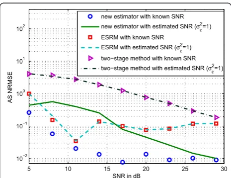
ESRM and the two-stage approach. However, for low SNR values, the new estimator shows higher NRMSE then the ESRM, when an estimate of the SNR is consid-ered. When the SNR is assumed known, the new esti-mator shows the best results (see Figure 11).

VI. Conclusion

In this article, we described a new low-complexity AS estimator for Rician fading channels. The new estimator first estimates the LOS component of the correlation coefficient. Then, the desired parameters are extracted from LUTs computed off-line. The estimate of the LOS component of the correlation coefficient requires the use of a K-factor estimator. The second- and fourth-order momentsK-factor estimator is considered for its simplicity and relatively good accuracy. To reduce the

0 1 2 3 4 5

10í2 10í1 100 101

K

AS NRMSE

new estimator with known SNR new estimator with estimated SNR (σ_ε2=1) ESRM with known SNR

ESRM with estimated SNR (σ_ε2₌₁₎

twoístage method with known SNR twoístage method with estimated SNR (σ_ε2=1)

Figure 9 NRMSE in AS using the butterfly configuration (Gaussian,_θm= 10°,sθ= 5°,SNRdB= 20 dB).

5 10 15 20 25 30

10í2 10í1 100 101 102

SNR in dB

AS NRMSE

new estimator with known SNR new estimator with estimated SNR (σ_ε2=1)

ESRM with known SNR ESRM with estimated SNR (σ_ε2₌₁₎

twoístage method with known SNR twoístage method with estimated SNR (σ_ε2=1)

Figure 11 NRMSE in AS using the butterfly configuration (Gaussian,_θm= 10°,sθ= 1°,K= 1,SNRdB= 20 dB).

0 2 4 6 8 10

10í2 10í1 100 101 102

σ_θ

AS NRMSE

new estimator with known SNR new estimator with estimated SNR (σ_ε2₌₁₎

ESRM with known SNR ESRM with estimated SNR (σ_ε2=1) twoístage method with known SNR twoístage method with estimated SNR (σ_ε2₌₁₎

Figure 10 NRMSE in AS using the butterfly configuration (Gaussian,θm= 10°,SNR= 20 dB,K= 1).

0 1 2 3 4 5

10í2 10í1 100

K

AS NRMSE

new estimator with known SNR new estimator with estimated SNR (σ_ε2₌₁₎

ESRM with known SNR ESRM with estimated SNR (σ_ε2=1) twoístage method with known SNR twoístage method with estimated SNR (σ_ε2₌₁₎

impact of the K-factor estimation error on AS estima-tion, the noise-induced biases in both the correlation coefficient and the moments of the received signal are reduced using an estimated SNR. The new estimator also includes a new method to select the angular distri-bution type of the received signal, which requires the use of a nonlinear array structure. The performance of the new method was compared with Spread Root-MUSIC extended to a nonlinear antenna array config-uration and with the two-stage approach presented in [13]. Simulations showed that the new technique gives lower NRMSE.

VII. Competing interests

The authors declare that they have no competing interests.

VIII. End notes a

The conventional array model described in [3] and [11] can be extended to a nonlinear structure by rewriting the associated steering vector. In this case, our problem can be reformulated using a matrix repre-sentation. However, this would only complicate the new algorithm by adding a new step for the determina-tion of the steering vector. That is why we consider the correlation coefficient of each antenna branch instead of the array formulation. b For each angular distribution type, there are two LUTs. The first is for the mean AoA, and the second is for the AS. c We rewrite the correlation coefficient for the different antenna pairs as in (8).

Abbreviations

AoA: angle of arrival; AS: angular spread; AWGN: additive white Gaussian noise; COE: contrast of eigenvalues; COMET: covariance matching estimation techniques; CRB: Cramér Rao bound; ESPRIT: estimation of signal parameters via rotational invariance techniques; ESRM: extended spread Root-MUSIC; LOS: line-of-sight; LS: least square; LUT: look-up table; ML: maximum likelihood; MUSIC; multiple signal classification; NLOS: Non-LOS; NRMSE: normalized mean square error; SIMO: single input-multiple output; SNR: signal-to-noise ratio; TLS: total least squares; ULA: uniform linear array; WLS: weighted least square

Acknowledgements

This article was presented in part at the IEEE Wireless Communications and Network Conference [14] and in the U.S. Patent Application no.

20070287385A1 [33].

Author details 1

Tunisian Polytechnic School, B.P. 743-2078, La Marsa, Tunisia2Wireless Communications Group, Institut National de la Recherche Scientifique, Centre Energie, Matériaux, et Télécommunications, 800, de la Gauchetiére Ouest, Bureau 6900, Montreal, QC, H5A 1K6, Canada3_{Huawei Technologies,} Markham, ON, Canada

Received: 27 October 2010 Accepted: 13 October 2011 Published: 13 October 2011

References

1. K Miyoshi, M Uesugi, U.S. Patent 20020123371A1

2. S Kikuchi, A Sano, H Tsuji, R Miura, A Novel Approach to Mobile-Terminal Positioning Using Single Array Antenna in Urban Environments, inIEEE VTS-Fall, vol. 58. (VTC, Orlando, 2003), pp. 1010–1014

3. S Valaee, B Champagne, P Kabal, Parametric localization of distributed sources. IEEE Trans Sig Process.43(9), 2144–2153 (1995). doi:10.1109/78.414777 4. Y Meng, P Stoica, KM Wong, Estimation of the directions of arrival of

spatially dispersed signals in array processing. IEEE Proc Inst Electron Eng Radar Sonar Navig.143(1), 1_–9 (1996). doi:10.1049/ip-rsn:19960170 5. M Bengtsson, B Ottersten, Low-complexity estimators for distributed sources.

IEEE Trans Sig Process.48(8), 2185–2194 (2000). doi:10.1109/78.851999 6. M Bengtsson, B Ottersten, A generalization of weighted subspace fitting to

full-rank models. IEEE Trans Sig Process.49(5), 1002–1012 (2001). doi:10.1109/78.917804

7. S Shahbazpanahi, S Valaee, MH Bastani, Distributed source localization using ESPRIT algorithm. IEEE Trans Sig Process.49, 2169_–2178 (2001). doi:10.1109/ 78.950773

8. S Shahbazpanahi, S Valaee, AB Gershman, A covariance fitting approach to parametric localization of multiple incoherently distributed sources. IEEE Trans Sig Process.52(3), 592–600 (2004). doi:10.1109/TSP.2003.822352 9. T Trump, B Ottersten, Estimation of nominal direction of arrival and angular

spread using an array of sensors. IEEE Trans Sig Process.45(1), 57–69 (1996) 10. T Trump, B Ottersten, Estimation of nominal direction of arrival and angular spread using an array of sensors. Sig Process.50, 57–69 (1996). doi:10.1016/ 0165-1684(96)00003-5

11. B Ottersten, P Stoica, R Roy, Covariance matching estimation techniques for array signal processing, Digit. Sig Process.8(3), 185_–210 (1998)

12. G Li, J Xu, Y Peng, X Xia, A low-complexity estimator for incoherently distributed sources with narrow or wide spread angles. Sig Process.87(5), 1058–1065 (2007). doi:10.1016/j.sigpro.2006.09.013

13. M Souden, S Affes, J Benesty, A two-stage approach to estimate the angles of arrival and the angular spreads of locally scattered sources. IEEE Trans Sig Process.56(5), 1968–1983 (2008)

14. I Bousnina, A Stéphenne, S Affes, A Samet, Performance of a New Low-Complexity Angular Spread Estimator in the Presence of Line-Of-Sight. IEEE Wireless Communications and Network Conference, 231_–236 (April 2008) 15. Y Jin, B Friedlander, Detection of distributed sources using sensor Arrays. IEEE Trans Sig Process.52(6), 1537_–1548 (2004). doi:10.1109/TSP.2004.827196 16. A Abdi, M Kaveh, A space-time correlation model for multi-element

antenna systems in mobile fading channels. IEEE J Select Areas Commun. 20(3), 550–560 (2002). doi:10.1109/49.995514

17. P Zetterberg, Mobile Cellular Communications with Base Station Antenna Arrays: Spectrum Efficiency, Algorithms and Propagation Models. Ph.D. Thesis, Signal Processing Department of Signals, Sensors and Systems, Royal Institute of Technology, Stockholm, Sweden (1997)

18. MR Spiegel,Schaum’s Mathematical Handbook of Formulas and Tables, (McGraw-Hill, USA, 1974)

19. K Kaouri,Left-Right Ambiguity Resolution of a Towed Array Sonar, (PhD. Thesis, Somerville College, University of Oxford, 2000)

20. M Hawkes, A Nehorai, Acoustic vector-sensor beamforming and capon direction estimation. IEEE Trans Sig Process.46(9), 2291–2304 (1998). doi:10.1109/78.709509

21. BC Liu, KH Lin, JY Chen, Ricean K-factor Estimation in Cellular

Communications Using Kolmogorov-Smirnov Statistic, APCC_‘06. Asia-Pacifc Conference on Communications, 1–5 (August 2006)

22. G Azemi, B Senadji, B Boashash, Ricean K-factor estimation in mobile communication systems. IEEE Commun Lett.8(10), 550–560 (2004) 23. Y Chen, NC Beaulieu, Maximum likelihood estimation of the K-factor in

ricean fading channels. IEEE Commun Lett.9(12), 1040–1042 (2005). doi:10.1109/LCOMM.2005.1576581

24. C Tepedelenlioglu, A Abdi, GB Giannakis, The Ricean K-factor: estimation and performance analysis. IEEE Trans Wirel Commun.2(4), 799–810 (2003) 25. C Tepedelenlioglu, A Abdi, GB Giannakis, M Kaveh, Performance Analysis of

Moment-Based Estimators for thekParameter of The Rice Fading Distribution. IEEE International Conference on Acoustics, Speech, and Signal Processing ICASSP’01.4, 2521–2524 (2001)

26. M Bakkali, A Stéphenne, S Affes, Generalized Moment-Based Method for SNR Estimation. inIEEE Wireless Communications and Networking Conference, WCNC, 2226–2230 (March 2007)

28. A Stéphenne, F Bellili, S Affes, Moment-Based SNR Estimation for SIMO Wireless Communication Systems Using Arbitrary QAM, inProceedings of 41st Asilomar Conference on Signals, Systems and Computers, ACSSC, 601_–605 (November 2007)

29. D Pauluzzi, N Beaulieu, A comparison of SNR estimation techniques for the AWGN channel. IEEE Trans Commun.48, 1681_–1691 (2000). doi:10.1109/ 26.871393

30. P Gao, C Tepedelenlioglu, SNR estimation for non-constant modulus Constellations. IEEE Trans Sig Process.53(3), 865–870 (2005)

31. F Belloni, A Richter, V Koivunen, Extension of Root-MUSIC to Non-ULA Array Configurations, Acoustics, Speech and Signal Processing, inICASSP 2006 Proceedings4, 897–900 (May 2006)

32. A Stéphenne, B Champagne, Effective multi-path vector channel simulator for antenna array systems. IEEE Trans Vehicul Technol.49(6), 2370–2381 (2000). doi:10.1109/25.901906

33. A Stéphenne, U.S. Patent 20070287385A1

doi:10.1186/1687-6180-2011-88

Cite this article as:Bousninaet al.:A new low-complexity angular spread estimator in the presence of line-of-sight with angular distribution selection.EURASIP Journal on Advances in Signal Processing

20112011:88.

Submit your manuscript to a

journal and benefi t from:

7Convenient online submission 7Rigorous peer review

7Immediate publication on acceptance 7Open access: articles freely available online 7High visibility within the fi eld

7Retaining the copyright to your article