A Comparative Study of Two Statistical Modelling Approaches
for Estimating Multivariate Likelihood Ratios
in Forensic Voice Comparison
Shunichi Ishihara
The Australian National University
Department of Linguistics
[email protected]
Abstract
The acoustic features used in forensic voice comparison (FVC) are correlated in almost all cases. A sizeable proportion of FVC studies and casework has relied, for statistical modelling, on the multivariate kernel density likelihood ratio (MVKDLR) formula, which considers the correlations between the features and computes an overall combined likelihood ratio (LR) for the offender-suspect com-parison. However, following concerns over the robustness of the MVKDLR, in particular its computational weakness and numerical instability specifically when a large number of features are employed, the principal component analysis kernel densi-ty likelihood ratio (PCAKDLR) approach was developed as an alternative. In this study, the performance of the two ap-proaches is investigated and compared us-ing Monte Carlo-simulated synthetic data based on the 16th-order Mel Frequency Cepstrum Coefficients extracted from the long vowel /e:/ segments of spontaneous speech uttered by 118 native Japanese male speakers. Performance is assessed in terms of validity (= accuracy) and reliabil-ity (= precision), with the log-likelihood ratio cost (Cllr) being used to assess
validi-ty and the 95% credible interval (95%CI) to assess reliability.
1
Introduction
In many branches of the forensic sciences, includ-ing finclud-ingerprint (Neumann et al., 2007), handwrit-ing (Marquis et al., 2011), voice (Morrison, 2009a), DNA (Evett et al., 1993), glass fragments (Curran, 2003), earmarks and footwear marks (Evett et al., 1998), strength of evidence is widely
measured using the LR framework, increasingly accepted as the standard framework for forensic inference and statistics. Calculating an LR for
voice evidence requires, as a first step, that each individual’s evidence (e.g. offender and suspect recordings) be modelled using various acoustic features (e.g. formant frequencies) that are corre-lated almost without exceptions. However, esti-mating an LR based on correlated variables is not a simple problem; it was addressed by Aitken and Lucy (2004), resulting in the development of the multivariate kernel density likelihood ratio (MVKDLR) approach. The MVKDLR has been extensively used, especially in acoustic-phonetic based forensic voice comparison (FVC) (Kinoshita et al., 2009; Morrison, 2009b), but was recently shown to be prone to instability, in par-ticular when the number of features for modelling is too high (e.g. features ≥ 5-6). The MVKDLR formula has the propensity to collapse when some of the covariance matrices of the offender and suspect data are ill-conditioned (e.g. sparse data, large number of input features) (Nair et al., 2014, pp. 90-91). This has motivated the development of an alternative, known as the principal component analysis kernel density likelihood ratio (PCAKDLR) approach (Nair et al., 2014).
To date, FVC studies in which the PCAKDLR is used to estimate LRs are limited; thus we don’t know how the PCAKDLR performs in compari-son to the MVKDLR (cf. Enzinger, 2016). To ad-dress this gap in our knowledge, the current study seeks to compare the performance of the MVKDLR and PCAKDLR approaches when the number of features for modelling changes, using synthetic data generated by Monte Carlo simula-tions (Fishman, 1995). The outcomes (scores) of the two approaches are calibrated using the lo-gistic-regression calibration technique proposed
by Brümmer and du Preez (2006). The perfor-mance of the approaches is assessed in terms of validity (= accuracy), for which the metric is the log-likelihood-ratio cost (Cllr) (Brümmer & du Preez, 2006), as well as reliability (= precision), for which the metric is the 95% credible interval (95%CI) (Morrison, 2011).
2
Likelihood Ratio
The likelihood ratio (LR), a measure of the quan-titative strength of evidence, is a ratio of two con-ditional probabilities: one is the probability (p) of observed evidence (E) assuming that one hypoth-esis (e.g. prosecution = Hp) is true; the other is the
probability of the same observed evidence assum-ing that the alternative hypothesis (e.g defence = Hd) is true (Robertson & Vignaux, 1995).Thus,
the LR can be expressed as 1).
In the case of FVC, the LR will be the proba-bility of observing the difference between the
of-fender’s and the suspect’s speech samples (re-ferred to as the evidence, E) if they had been produced by the same speaker (Hp) relative to the
probability of observing the same evidence (E) if they had been from different speakers (Hd). The
relative strength of the given evidence with re-spect to the competing hypotheses (Hp vs. Hd) is
reflected in the magnitude of the LR. The more the LR deviates from unity (LR = 1; logLR = 0), the greater support for either the prosecution pothesis (LR > 1; logLR > 0) or the defence hy-pothesis (LR < 1; logLR < 0).
The important point is that the LR is con-cerned with the probability of the evidence, giv-en the hypothesis (either Hp or Hd), which is the
province of forensic scientists, while the trier-of-fact is concerned with the probability of the hy-pothesis, given the evidence. That is, the ultimate decision as to whether the suspect is guilty or not does not lie with the forensic expert, but with the court. The role of the forensic scientist is to esti-mate the strength of evidence (= LR) with a view to help the trier-of-fact make a final decision (Morrison, 2009a, p. 229).
3
Database, target segment, and
speak-ers
In this study, monologues from the Corpus of Spontaneous Japanese (CSJ) (Maekawa et al.,
2000) are used for FVC experiments. The record-ings are 10-25 minutes long.
For this study, it was decided to target fillers. Fillers are sounds or words (e.g. um, you know, like in English) uttered by a speaker to signal that he/she is thinking or hesitating. The filler /e:/ and the /e:/ segment of the filler /e:to:/ were chosen because i) they are two of the most frequently used fillers in Japanese (many monologues con-tain at least ten of them) (Ishihara, 2010), ii) the vowel /e/ reportedly has the strongest speaker-discriminatory power out of the five Japanese vowels /i,e,a,o,u/ (Kinoshita, 2001), and iii) the segment /e:/ is significantly long so that it is easy to extract stable spectral features from this seg-ment. It is also considered that fillers are uttered unconsciously or semiconsciously by the speaker and carry no lexical meaning. They are thus not likely to be affected by the pragmatic focus of the utterance.
For the experiments, speakers were selected from the CSJ based on five criteria: i) availability of two non-contemporaneous recordings per speaker (n.b. suspect and offender recordings are non-contemporaneous in real cases), ii) high only male speakers were chosen for experiments. This is because males are more likely to commit crimes than females (Kanazawa & Still, 2000). The five criteria combined resulted in 236 re-cordings (118 speakers x 2 non-contemporaneous recordings), all of which were used in our experiments.
The 118 speakers were divided into three mu-tually exclusive sub-databases: the test database (40 speakers), the background database (39 speakers) and the development database (39 speakers). Each speaker in these databases has two recordings that are non-contemporaneous. The first ten /e:/ segments were annotated in each recording. Thus, for example, there are 800 an-notated /e:/ segments in the test database (= 40 speakers x 2 sessions x 10 segments). Data spar-sity is a common issue in FVC. Ten samples for each recording can be judged as a realistic set-ting. All statistics required for conducting Monte Carlo simulations were calculated using these da-tabases.
The speaker comparisons derived from the test database were used to assess the performance of the FVC system. The background database was
LR=p(E|Hp)
used as a background reference population, and the development database was for obtaining the logistic-regression weight, which was used to calibrate the scores of the test database (refer to §4.5 for a detailed explanation of calibration).
4
Experiments
4.1 FeaturesWe used 16 Mel Frequency Cepstrum Coeffi-cients (MFCC) in the experiments as feature vec-tors. MFCC is a standard spectral feature used in many voice-related applications, including auto-matic speaker recognition. All original speech samples were downsampled to 16kHz before MFCC values were extracted from the mid-duration-point of the target segment /e:/ with a 20 ms wide hamming window.
4.2 General experimental design
There are two types of tests for FVC. One relies on so-called Same Speaker Comparisons (SS comparisons), where two speech samples pro-duced by the same speakers are compared. They are expected to receive LR values > 1 given the same-origins. The other type of test relies on Dif-ferent Speaker Comparisons (DS comparisons), where two speech samples produced by different speakers are compared. They are expected to re-ceive LR values < 1 given the different-origins.
For example, the 40 speakers of the test data-base enable us to undertake 40 SS comparisons and 1560 (= 50C2 x 2) independent (e.g.
not-overlapping) DS comparisons. Theoretically speaking, origin being identical, the 40 SS com-parisons should receive an LR > 1 (log10LR > 0);
on the other hand, origin being different, the 1560 DS comparisons should receive an LR < 1 (or log10LR < 0).
4.3 Likelihood ratio calculation MVKDLR Approach
The MVKDLR formula computes a single LR from multiple variables (e.g. 16th-order MFCC),
considering the correlations among them (Aitken & Lucy, 2004).
The numerator of the MVKDLR formula cal-culates the probability of evidence, which is the difference between the offender and suspect speech samples, when it is assumed that both samples have the same origin (in other words,
that the persecution hypothesis Hp is true). For
this calculation, the feature vectors of the
offend-er and suspect samples and the within-speaker
variance, which is given in the form of a vari-ance/covariance matrix, are needed. The same feature vectors of the offender and suspect
sam-ples and the between-speaker variance are used
in the denominator of the formula to estimate the probability of getting the same evidence when it is assumed that they have different origins (i.e.
that the defence hypothesis Hd is true). These
within- and between-speaker variances are esti-mated from the background database. The MVKDLR formula assumes normality for with-in-speaker variance while it uses a kernel-density model for between-speaker variance.
In the MVKDLR formula, the covariance ma-trices for offender and suspect data are used ex-tensively. The inverses of these matrices are re-quired at some stages in the process, and there are also some instances of these inverted matri-ces being re-inverted. All of these promatri-cesses con-tribute to the decorrelation of the original fea-tures and the equalisation of their contribution. However, in return, the MVKDLR formula has the propensity to collapse when some of the co-variance matrices of the offender and suspect da-ta are ill-conditioned due to, for example, sparse data and large input parameters.
PCAKDLR Approach
In the PCAKDLR approach, in particular when high-dimensional features are used, the issue of the instability described for the MVKDLR is han-dled by decorrelating the features through princi-pal component analysis (PCA), and then estimat-ing LRs as the product of the univariate LRs of the resultant uncorrelated features. Thus, PCA is merely used to decorrelate the features (not to re-duce feature dimensionality). With the resultant orthogonal features, a univariate LR was estimat-ed separately for each feature using the modifiestimat-ed kernel density model (Nair et al., 2014, pp. 88
-90); the independent LRs were multiplied to gen-erate an overall LR.
4.4 Repeated experiments using Monte Car-lo simulations
As explained earlier, each speaker has two sets of ten /e:/ segments, and 16 MFCC values were ex-tracted from each of them. That is, each session of each speaker can be modelled maximally with ten sets of 16th-order feature vectors. From these ten
for the Monte Carlo simulations. In this study, we randomly generated, for each session of each speaker, ten feature vectors, each of which con-sists of 16 MFCC values. We repeated this proce-dure 150 times using the normal distribution func-tion modelled with the basic statistics.
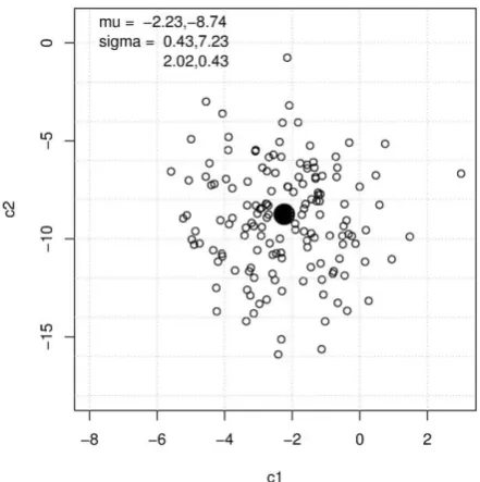
Figure 1 is an example of the Monte Carlo simulation showing 150 randomly generated first two MFCC values (c1 and c2) from the normal distribution function based on the statistics ( and ) obtained from the first session of the first speaker in the test database.
Figure 1: 150 randomly generated values (c1 and c2) from the statistics ( and ) obtained from the first session of the first speaker in the test database (only the first and second MFCC). The filled black circle =
.
Experiments were repeatedly conducted using randomly generated synthetic feature vectors with different dimensions (= {2,4,6,8,10,12,14,16}). For example, a feature dimension of {2} means that the first two MFCC values were used for experiments, and a feature dimension of {14} means that the first 14 MFCC were used.
4.5 Calibration
A logistic-regression calibration (Brümmer & du Preez, 2006) was applied to the outputs (scores) of the MVKDLR and PCAKDLR approaches. Given two sets of scores derived from the SS and DS comparisons and a decision boundary, cali-bration is a normalisation procedure involving linear monotonic shifting and scaling of the scores relative to the decision boundary, so as to
minimise a cost function, resulting in LRs. The FoCal toolkit 1 was used for the
logistic-regression calibration in this study (Brümmer & du Preez, 2006). The logistic-regression weight was obtained from the development database.
4.6 Evaluation of performance: validity and reliability
The performance of the LR-based FVC system needs to be assessed in terms of its validity (= accuracy) and reliability (= precision). To ex-plain the concepts of validity and reliability, we will look at an example. Let us imagine we have speech samples collected from two speakers at four different sessions denoted as S1.1, S1.2, S1.3, S1.4, S2.1, S2.2, S2.3 and S2.4, where S = speaker, and 1, 2, 3 and 4 = the first, second, third and fourth sessions (e.g. S1.1 refers to the first session recording collected from (S)peaker1, and S1.4 to the fourth session from that same speaker). From these speech samples, four inde-pendent (not overlapping) DS comparisons are possible: S1.1 vs. S2.1, S1.2 vs. S2.2, S1.3 vs. S2.3 and S1.4 vs. S2.4. Let us further suppose that we conducted two separate FVC tests using two different systems (Systems 1 and 2), and that we obtained the log10LRs given in Table 1 for
these four DS comparisons.
Since the comparisons given in Table 1 are all DS comparisons, the desired log10LR value needs
to be lower than 0, and the greater the negative log10LR value is, the better the system is, as it
more strongly supports the correct hypothesis. For both Systems 1 and 2, all of the comparisons received log10LR < 0. That is, all of these
log10LR values correctly single out the defence
hypothesis. However, System 1 performs better than System 2 in that its log10LR values are
fur-ther away from unity (log10LR = 0) than the
log10LR values of System 2. This means that the
log10LR values estimated by System 1 provide
greater support for the correct hypothesis than System 2. Thus, it can be said that the validity (=
1 https://sites.google.com/site/nikobrummer/focal
DS comparison System 1 System 2 S1.1 vs. S2.1 -8.3 -5.1 S1.2 vs. S2.2 -7.9 -1.2 S1.3 vs. S2.3 -8.0 -3.1
S1.4 vs. S2.4 -8.2 -0.1 Table 1: Example log10LRs explaining the concepts of
accuracy) of System 1 is higher than that of Sys-tem 2. This is the basic concept of validity.
In this study, the log-likelihood-ratio cost (Cllr), which is a gradient metric based on LR, was used as the metric for validity. The calcula-tion of Cllr is given in 2) (Brümmer & du Preez,
LRs derived from the SS and DS comparisons, re-spectively. Given the same origins, all the SS comparisons should produce LRs greater than 1, and given the different origins, the DS compari-sons should produce LRs less than 1. Cllr takes in-to account the magnitude of derived LR values, and assigns them appropriate penalties. In Cllr, LRs that support counter-factual hypotheses or, in other words, contrary-to-fact LRs (LR < 1 for SS comparisons and LR > 1 for DS comparisons) are heavily penalised and the magnitude of the penal-ty is proportional to how much the LRs deviate from unity. The lower the Cllr value, the better the performance.
The Cllr measures the overall performance of a system in terms of validity based on a cost func-tion in which there are two main components of loss: namely discrimination loss (Cllrmin) and cali-bration loss (Cllrcal) (Brümmer & du Preez, 2006). The former is obtained after the application of the so-called pooled-adjacent-violators (PAV) trans-formation – an optimal non-parametric calibration procedure. The latter is obtained by subtracting the former from the Cllr. In this study, besides Cllr, Cllrmin and Cllrcal are also referred to. Once again, the FoCal toolkit1 was used in this study for
calcu-lating Cllr (including both Cllrmin and Cllrcal) (Brümmer & du Preez, 2006).
Let us now move to the concept of reliability. All of the DS comparisons given in Table 1 are comparisons of the same speaker pair (S1 vs. S2). Thus, it can be expected that the LR values ob-tained for these four DS comparisons should be similar as they are comparing the same speaker pair. However, the log10LR values based on
Sys-tem 1 are closer to each other (-8.3, -7.9, -8.0 and
-8.2) than those based on System 2 (-5.1, -1.2, -3.1 and -0.1). In other words, the reliability (=
preci-sion) of System 1 is higher than that of System 2. This is the basic concept of reliability.
As a metric of reliability, we used 95%credible intervals, the Bayesian analogue of frequentist confidence intervals (Morrison, 2011). In this study, we calculated 95% credible intervals (95%CI) in the parametric manner based on the deviation-from-mean values collected from all of the DS comparison pairs. For example, 95%CI = 1.23 and log10LR = 2 means, for this particular
comparison, that it is 95% certain that log10LR >
0.77 (= 2-1.23) and log10LR < 3.23 (= 2+1.23).
The smaller the 95%CI, the better the reliability. The 95%CI is obtainable only from the DS com-parisons in the present study.
5
Experiment with Original Data
Before presenting the results of the experiments using synthetic data, we conducted experiments using the full 16th-order MFCC values from the
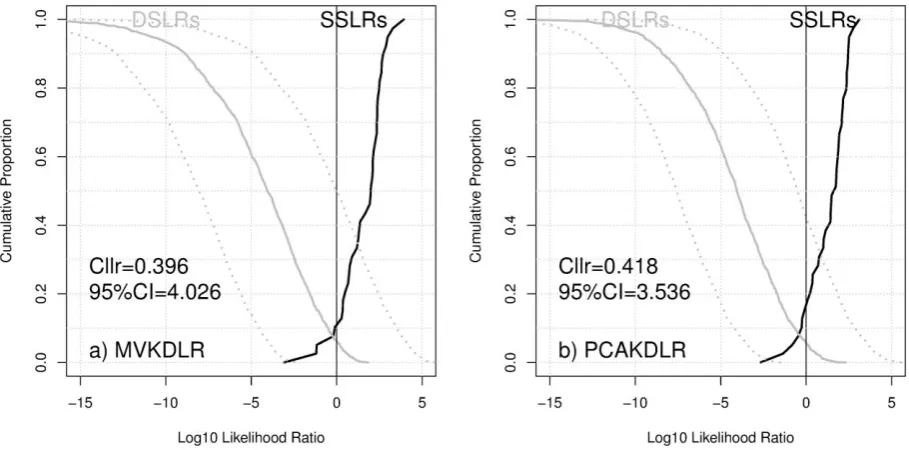
original databases with the two different ap-proaches. The results of these experiments are given as Tippett plots in Figure 2 with the Cllr and 95%CI values. Figure 2a is for the MVKDLR and Figure 2b is for the PCAKDLR. In these Tippett plots, the solid black curve indicates the cumula-tive proportion of the SS comparison log10LRs
(40) that are equal or smaller than the value indi-cated on the x-axis, and the solid grey curve indi-cates the cumulative proportion of the DS com-parison log10LRs (1560) that are equal or greater
than the value indicated on the x-axis. Tippett plots graphically show how strongly the derived LRs not only support the correct hypothesis but also misleadingly support the contrary-to-fact hy-pothesis. In Figure 2, the log10LRs for the DS
comparisons are plotted together with 95%CI band.
metric value, they are virtually the same and therefore comparable.
6
Experimental Results and Discussions
It was shown in §5 that, in terms of the Cllr (in-cluding both Cllrmin and Cllrcal), the MVKDLR per-formed marginally better than the PCAKDLR (they performed equally well in a practical sense), but that the PCAKDLR outperformed the MVKDLR in terms of the 95%CI. It will be in-vestigated in this section whether the observation made in §5 is a general observation that retains its validity when synthetic data are used. It will also be investigated how the number of features affects the performance of the two different approaches because the MVKDLR reportedly has an issue of instability when high-dimensional features are used.
Before the results of the experiments are dis-played, it needs to be pointed out that the Cllr (MVKDLR = 0.396 and PCAKDLR = 0.418) and 95%CI values (MVKDLR = 4.026 and PCAKDLR = 3.536) with the 16th-order MFCC
feature vector of the original data, which were given in §5, are similar to the mean Cllr (MVKDLR = 0.439 and PCAKDLR = 0.465) and 95%CI values (MVKDLR = 0.3348 and PCAKDLR = 2.689) of the 150 simulations with the synthetic 16th-order MFCC feature vector. This
suggests the appropriateness of the Monte Carlo simulation.
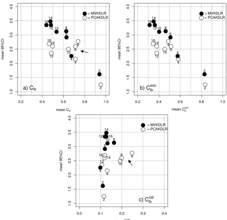
In Figure 3, the mean Cllr (Panel a), Cllrmin (Pan-el b) and Cllrcal (Panel c) values of the 150 simula-tions are plotted for the different feature numbers (= {2,4,6,8,10,12,14,16}) against the mean 95%CI values (y-axis), but separately for the MVKDLR (filled circles) and PCAKDLR (empty circles) ap-proaches. The numerical information of Figure 3 is given in Table 2.
It can be seen from Figure 3a that the overall performance of the MVKDLR in terms of validity (Cllr) improves as the number of features increases in that there is substantial improvement when moving from two to four features (from Cllr = 0.939 for {2} to Cllr = 0.674 for {4}), after which the improvement still continues, yet to a substan-tially lesser degree. The general trend of the relia-bility (95%CI) for the MVKDLR is that it deterio-rates as the feature number increases. Thus, the trade-off between validity and reliability is fairly clearly observable in the case of the MVKDLR. Although, in terms of validity, the PCAKDLR shows a more or less similar trend compared to the MVKDLR, some exceptions (e.g. the feature number = {6,8}) can also be observed in that the inclusion of additional features did not contribute to an improvement in validity (from Cllr = 0.712 for {6} to Cllr = 0.736 for {8}). These exceptions Figure 2: Tippett plots showing the magnitude of the derived LRs plotted separately for the SS (black) and DS (grey) comparisons. 95%CI bands (grey dotted lines) are superimposed on the DS LRs. Panel a = MVKDLR and Panel b = PCAKDLR. Cllr value was calculated from the calibrated LRs and 95%CI value was calculated only for
will be further investigated below with reference to calibration loss (Cllrcal).
The main difference between the two ap-proaches that can be observed from Figure 3a is that the inverse-correlation identified between va-lidity and reliability for the MVKDLR is not
clearly observable in the case of the PCAKDLR; the 95%CI values stay relatively constant around a 95%CI = 2.5 when six or more features are used for the experiments. As a result, although the PCAKDLR is constantly better in reliability (95%CI) than the MVKDLR, reliability is consid-erably better for the former than for the latter, in particular when the feature number is large
(fea-ture number ≥ 5-6). The observations derived from Figure 3a above more or less coincide with Enzinger (2016) finding that the MVKDLR is su-perior to the PCAKDLR in terms of validity, but inferior in terms of reliability.
Close observation of Figure 3b, which plots the discriminability of the system (Cllrmin) against its reliability shows an even clearer difference be-tween the MVKDLR and PCAKDLR approaches described on the basis of Figure 3a in that the 95%CI values seem to hit a ceiling with six fea-tures or more for the PCAKDLR, while the 95%CI value continues to increase for the MVKDLR as a function of the feature number. Figure 3: Mean Cllr (Panel a), Cllrmin (b) and Cllrcal (c) values (x-axis) plotted against mean 95%CI values (y-axis). Filled and empty circles = MVKDLR and PCAKDLR, respectively. The number attached to each circle indicates the dimension of the feature vector. Note that the range of the x-axis scale is narrower for Panel c) than for Panels
Figure 3b shows that i) system discriminability improves as a function of the number of features both for the MVKDLR and PCAKDLR ap-proaches, ii) discriminability is marginally but constantly better for the MVKDLR, and iii) relia-bility is constantly better for the PCAKDLR; the former is considerably better than the latter when the feature number is large (feature number ≥ 6).
From Figure 3c, it can be seen that calibration performance is fairly constant and comparable (ca. Cllrmin = 0.125) between the MVKDLR and PCAKDLR approaches across different feature numbers, except for feature number = {6,8,10} for the PCAKDLR, which is indicated by an arrow in Figure 3c. The poor performance in calibration for feature numbers = {6,8,10} of the PCAKDLR contributes to the overall poor Cllr values of the PCAKDLR for the same feature numbers, which can be clearly seen in Figure 3a (as indicated by the arrow). As a result, the Cllr values of feature numbers = {6,8,10} are fairly better for the MVKDLR than for the PCAKDLR, while the former approach is only marginally better than the latter for the other feature numbers. However, it is not clear at this stage whether these poor calibra-tions are due to the PCAKDLR approach or other intrinsic or extrinsic reasons.
It has been reported in some studies that validi-ty and reliabilivalidi-ty are often (but not always) nega-tively correlated (Frost, 2013; Ishihara, 2017; Morrison, 2011). That is, the better performance of the PCAKDLR in reliability may be merely due to the trade-off between validity and reliabil-ity because the MVKDLR performs better than the PCAKDLR in terms of validity. Although the effect of the trade-off should not be neglected, it is true that the PCAKDLR is substantially better in reliability than the MVKDLR, while the MVKDLR only marginally performed better than the PCAKDLR in terms of discriminability. The general trend for the 95%CI value to continue to
increase as the feature number increases is another aspect of the MVKDLR that the PCAKDLR does not exhibit; the 95%CI values become saturated with a feature number ≥ 6. Thus, it is a sensible conclusion that the PCAKDLR is better than the MVKDLR in terms of reliability.
7
Conclusions and Future Directions
The outcomes of the experiments with the simu-lated data demonstrate some general characteris-tics of the PCAKDLR approach as compared to the MVKDLR approach: i) the PCAKDLR ap-proach marginally underperforms the MVKDLR approach in terms of discriminability (Cllrmin), ii) the PCAKDLR approach performs constantly bet-ter than the MVKDLR in bet-terms of reliability, and iii) a substantial difference in reliability perfor-mance can be observed in particular when the fea-ture number is six or more. In some cases, the MVKDLR performed noticeably (not marginally) better than the PCAKDLR (e.g. feature number = {6,8,10}) with respect to Cllr, but it was pointed out that this is due to the poor calibration perfor-mance of the PCAKDLR. However, it is not clear whether these poor calibrations are indeed caused by the PCAKDLR or by other unrelated factors.
In the current study, the maximum number of /e:/ tokens, which is ten, was used to model each session of each speaker. It would be interesting to explore how a different number of tokens for modelling will influence the performance of the MVKDLR and PCAKDLR approaches because, in real cases, one is less likely to have many com-parable tokens for modelling.
Acknowledgments
The author thanks the three reviewers for their valuable comments.
Metrics Approaches 2 4 6 8 10 12 14 16
Cllr MVKDLR PCAKDLR 0.939 0.950 0.674 0.712 0.712 0.628 0.626 0.736 0.534 0.646 0.485 0.482 0.497 0.477 0.439 0.465
Cllrmin MVKDLR PCAKDLR 0.834 0.828 0.576 0.581 0.508 0.513 0.462 0.488 0.454 0.401 0.379 0.361 0.379 0.350 0.312 0.345
Cllrcal MVKDLR PCAKDLR 0.115 0.110 0.098 0.131 0.120 0.198 0.163 0.248 0.192 0.132 0.106 0.120 0.118 0.127 0.127 0.120
95%CI MVKDLR PCAKDLR 1.615 1.250 2.258 2.148 2.595 2.915 3.132 2.771 3.112 2.498 2.360 3.348 2.603 3.478 3.348 2.689
References
Aitken, C. G. G., & Lucy, D. (2004). Evaluation of trace evidence in the form of multivariate data. Journal of the Royal Statistical Society, Series C (Applied Statistics), 53(1), 109-122.
Brümmer, N., & du Preez, J. (2006). Application-independent evaluation of speaker detection. Computer Speech and Language, 20(2-3), 230-275.
Curran, J. M. (2003). The statistical interpretation of forensic glass evidence. International Statistical Review, 71(3), 497-520.
Enzinger, E. (2016). Likelihood ratio calculation in acoustic-phonetic forensic voice comparison: Comparison of three statistical modelling approaches. Proceedings of the Interspeech 2016, 535-539.
Evett, I. W., Lambert, J. A., & Buckleton, J. S. (1998). A Bayesian approach to interpreting footwear marks in forensic casework. Science & Justice, 38(4), 241-247.
Evett, I. W., Scranage, J., & Pinchin, R. (1993). An illustration of the advantages of efficient statistical-methods for RFLP analysis in forensic-science. American Journal of Human Genetics, 52(3), 498-505.
Fishman, G. S. (1995). Monte Carlo: Concepts, Algorithms, and Applications. New York: Springer.
Frost, D. (2013). Likelihood Ratio-based Forensic Voice Comparison on L2 Speakers: A Case of Hong Kong Male Production of English Vowels. (Unpublished Honours thesis), The Australian National University, Canberra.
Ishihara, S. (2010). Variability and consistency in the idiosyncratic selection of fillers in Japanese monologues: Gender differences. Proceedings of
the Australasian Language Technology
Association Workshop 2010, 9-17.
Ishihara, S. (2017). Strength of forensic text comparison evidence from stylometric features: A multivariate likelihood ratio-based analysis. The International Journal of Speech, Language and the Law, 24(1), 67-98.
Kanazawa, S., & Still, M. C. (2000). Why men commit crimes (and why they desist). Sociological Theory, 18(3), 434-447.
Kinoshita, Y. (2001). Testing Realistic Forensic Speaker Identification in Japanese: A Likelihood
Ratio Based Approach Using Formants.
(Unpublished PhD thesis), The Australian National University, Canberra.
Kinoshita, Y., Ishihara, S., & Rose, P. (2009). Exploring the discriminatory potential of F0 distribution parameters in traditional forensic speaker recognition. International Journal of Speech Language and the Law, 16(1), 91-111.
Maekawa, K., Koiso, H., Furui, S., & Isahara, H. (2000). Spontaneous speech corpus of Japanese. Proceedings of the 2nd International Conference of Language Resources and Evaluation, 947-952. Marquis, R., Bozza, S., Schmittbuhl, M., & Taroni, F.
(2011). Handwriting evidence evaluation based on the shape of characters: Application of multivariate likelihood ratios. Journal of forensic sciences, 56(Supplement 1), S238-242.
Morrison, G. S. (2009a). Forensic voice comparison and the paradigm shift. Science & Justice, 49(4), 298-308.
Morrison, G. S. (2009b). Likelihood-ratio forensic voice comparison using parametric representations of the formant trajectories of diphthongs. Journal of the Acoustical Society of America, 125(4), 2387-2397.
Morrison, G. S. (2011). Measuring the validity and reliability of forensic likelihood-ratio systems. Science & Justice, 51(3), 91-98.
Nair, B., Alzqhoul, E., & Guillemin, B. J. (2014). Determination of likelihood ratios for forensic voice comparison using principal component analysis. International Journal of Speech Language and the Law, 21(1), 83-112.
Neumann, C., Champod, C., Puch-Solis, R., Egli, N., Anthonioz, A., & Bromage-Griffiths, A. (2007). Computation of likelihood ratios in fingerprint identification for configurations of any number of minutiae. Journal of forensic sciences, 52(1), 54-64.