Optimal Redundancy Allocation in Complex Systems

(1)

IJEDR1603110

International Journal of Engineering Development and Research (www.ijedr.org)

672

Optimal Redundancy Allocation in Complex

Systems

1

_{Chandan Choubey,}

2

_{Abhas Kanungo,}

3

_{Piyush Chandra Ojha,}

4

_{Ajeet Pratap Singh}

1_{Assistant Professor,}2_{Assistant Professor,}3_{Assistant Professor}

1_{Electronics & Instrumentation Department,}

1_{Krishna Institute of Engineering & Technology, Ghaziabad, India}

________________________________________________________________________________________________________

Abstract—A simple computational procedure has been developed by using Monte Carlo for allocating redundancy among subsystems so as to achieve maximum reliability of a complex systems subjected to multiple constraints which may be linear, non linear separable or non separable. Two examples of linear, non linear separable and non separable constraints with having twenty problems are solved.

Index Terms— Active Redundancy, System Reliability, Constraints, Problem formulation, Monte Carlo Algorithm.

________________________________________________________________________________________________________

I.INTRODUCTION

Reliability of an overall system can be increased by introducing redundancies in subsystems. In order to ensure that factors such as cost, weight, and volume remain within resources available, system reliability is optimized with respect to these constraints. The redundancy optimization problem is a classical problem that has attracted considerable attention from the research community. It has been solved by using optimization approaches and techniques such as dynamic programming[1], integer programming[3], mixed-integer linear programming[2], heuristics[4] and meta-heuristics[5] which gives either optimal or very good solutions.

This paper presents a Monte Carlo Method [6] that solves the problems of constrained redundancy optimization in complex system which gives the local optimal system reliability. Our aim is to show how to maximize system reliability subjected to the given constraints. For optimizing the system reliability we prefer simulation because it gives the result fast & accurate.

For solving this problem (or optimizing system reliability) many authors have used cumbersome approaches. However in this paper the proposed Monte Carlo Method is applied for all systems and to all type of constraints and also it has been tried on many problems, with satisfactory results.

II. PROBLEM FORMULATION AND COMPUTATION PROCEDURE

A. Notations

 Ri(xi), Qi(xi) reliability, unreliability of subsystem-i with xi components.  Rs(x) system reliability

 xi number of components in subsystem-i  x (x1,... xn)

 x*(ru) optimum value of x in iteration u

 Gir (xi) resource-r consumed in subsystem-i with xi components.  br maximum of resource-r

 k number of constraints  n number of subsystems

 f(.) function that yields the system reliability, based on n unique, subsystems and which depends on the configuration of the subsystems.

 αl (x) Sensitivity-factor  bi(xi) Selection-factor

 p1 Minimal path Set-l of the system  ci Cost of the xi subsystem

B. Assumptions

 The system and all of its subsystems are coherent.

 There are n subsystems in the system. Subsystem structure (other than coherence) is not restricted.  All component states are mutually statistically in dependent.

 All constraints are separable and additive among components. Each constraint is an increasing function of xi for each subsystem.

(2)

IJEDR1603110

673

C. Problem Formulation

 The problem of constrained redundancy optimization in complex systems can be reduced to the following integer programming problem:

 Maximize: Rs(x) = f ( R1(x1),...,Rn(xn) )  Subject to multiple linear or nonlinear constraints :

∑𝑘𝑖=1𝐺ᵢᵣ(𝑥) ≤ 𝑏ᵣ; r = 1,2,3...s where the 𝑥ᵢ are positive integers, for all i

III. MONTE CARLO ALGORITHM

Steps of Algorithm 1. Let xi =1 for all i 2. Calculate Rs(x) 3. Repeat 100 times

𝑥𝑖∗ = random number between 1 to 10 for all i.

Both linear and nonlinear (∑𝑘𝑖=1𝐺ᵢᵣ(𝑥ᵢ) ≤ 𝑏ᵣ) are violated. If no constraint are violated Calculate Rs(x*)

If Rs(x*) ≥ Rs(x)

Then Rs(x) = Rs(x*) at x = x* Calculate the output 𝑥𝑖∗, G(𝑥) and Rs(𝑥)

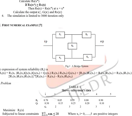
4. The simulation is limited to 3000 iteration only

IV.FIRST NUMERICAL EXAMPLE [7]

Fig.1 A Bridge System The expression of system reliability (Rs) is

Rs(x) = R1(x1 )R2(x2)Q3(x3)Q5(x5) + Q1(x1) R3(x3) R4(x4) Q5(x5) + [R1(x1)R3(x3) + R3(x3)R5(x5) + R5(x5)R1(x1) – 2R1(x1)R3(x3)R5(x5)] *[R2(x2) + R4(x4) - R2(x2)R4(x4)

A. Problem

TABLE 1

Shows subsystem’s data

i 1 2 3 4 5

Rᵢ 0.70 0.85 0.75 0.80 0.90 Qi 0.30 0.15 0.25 0.20 0.10

cᵢ 2 3 2 3 1 Maximize Rs(x)

Subjected to linear constraints ∑𝟓 𝐜ᵢ𝐱ᵢ

𝒊=𝟏 ≤ 20 Where xi, i= 0,...,5 are positive integers B. Solution

TABLE 2

Shows the optimal solution after particular Iteration

Ri 0.70 0.85 0.75 0.80 0.90 ∑cixi Rs(x) Iteration (u) Qi 0.30 0.15 0.25 0.20 0.10

20 0.9949 2400

ci 2 3 2 3 1

xi 1 2 4 1 1

cixi 2 6 8 3 1

(3)

IJEDR1603110

674

The above table shows the result of Monte Carlo Simulation. At 2400 iteration we get best combination of redundancy (x1,...x5), which satisfy the given constraints, It means the optimal solution is x*= {1,2,4,1,1} and Rs(x*) = 0.994

V.

TWENTY DIFFERENT SETS OF PROBLEM

Twenty different data sets are considered and are solved by the proposed algorithm to obtain the best combination of redundancy (xi) and system reliability (Rs).

A. Problems

TABLE 3

Shows the cost of the subsystems

Cost (ci) c1 c2 c3 c4 c5

2 3 2 3 1

TABLE 4

Shows the subsystem’s reliability and consumed resources

Problem No. R1(x1) R2(x2) R3(x3) R4(x4) R5(x5) ∑𝟓_𝒊=𝟏𝐜ᵢ𝐱ᵢ≤

1 0.70 0.85 0.75 0.80 0.90 20

2 0.60 0.70 0.80 0.90 0.60 30

3 0.70 0.85 0.90 0.80 0.75 30

4 0.70 0.85 0.90 0.80 0.75 35

5 0.80 0.80 0.90 0.90 0.90 25

6 0.80 0.80 0.90 0.90 0.90 30

7 0.80 0.80 0.90 0.90 0.90 35

8 0.75 0.65 0.85 0.95 0.55 20

9 0.75 0.65 0.85 0.95 0.55 25

10 0.75 0.65 0.85 0.95 0.55 30

11 0.80 0.65 0.72 0.78 0.60 25

12 0.80 0.65 0.72 0.78 0.60 30

13 0.80 0.65 0.72 0.78 0.60 34

14 0.90 0.90 0.75 0.75 0.75 25

15 0.90 0.90 0.75 0.80 0.75 25

16 0.90 0.90 0.75 0.80 0.75 30

17 0.72 0.62 0.59 0.93 0.67 25

18 0.72 0.62 0.59 0.93 0.67 30

19 0.72 0.62 0.59 0.93 0.67 35

20 0.95 0.67 0.59 0.93 0.67 30

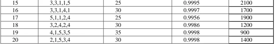
B. Solutions

TABLE 5

Shows Optimal Redundancy and system reliability for the given problems

Problem no. Redundancy {xi} Consumed Resources (∑cixi) Reliability (RS(xi)) Iteration (u)

1 1,2,4,1,1 20 0.9949 2600

2 1,2,5,3,3 30 0.9998 1900

3 4,2,1,4,2 30 0.9991 2100

4 5,3,3,3,1 35 0.99996 1700

5 3,1,1,4,2 25 0.9990 2700

6 2,3,3,3,2 30 0.9999 1600

7 4,1,4,4,4 35 0.99996 800

8 3,1,2,2,1 20 0.9953 2600

9 4,2,1,2,3 25 0.9974 2300

10 2,3,5,2,1 30 0.9998 1500

11 3,1,2,3,3 25 0.9939 2300

12 2,2,3,3,5 30 0.9978 1100

13 1,2,5,5,1 34 0.9995 900

(4)

IJEDR1603110

675

15 3,3,1,1,5 25 0.9995 2100

16 3,3,1,4,1 30 0.9997 1700

17 5,1,1,2,4 25 0.9956 1900

18 3,2,4,2,4 30 0.9986 1200

19 4,1,5,3,5 35 0.9998 900

20 2,1,5,3,4 30 0.9998 1400

VI.SECOND NUMERICAL EXAMPLE

Fig.2 A Complex System (5 nodes, 7edges) The system reliability (RS) equation is

RS(X) =(𝑄₆𝑥₆)[(1-𝑄₁𝑥₁)(1-𝑄₂𝑥₂)(1-𝑄₃𝑥₃)(𝑄₇𝑥₇)(𝑄₄𝑥₄)+(𝑄₁𝑥₁)(𝑄₂𝑥₂)(1-𝑄₄𝑥₄)(1-𝑄₅𝑥₅)(𝑄₇𝑥₇)+[(1-𝑄₁𝑥₁)(1-𝑄₂𝑥₂)(1-𝑄₄𝑥₄)+(1-𝑄₄𝑥₄ )(1-𝑄₇𝑥₇_)+(1-𝑄₇𝑥₇_(1-𝑄₁𝑥₁_)(1-𝑄₂𝑥₂_{)-2(1-𝑄₁}𝑥₁_)(1-𝑄₂𝑥₂_)(1-𝑄₄𝑥₄_)(1-𝑄₇𝑥₇_{)][(1-𝑄₃}𝑥₃_)+(1-𝑄₅𝑥₅_)-(1-𝑄₃𝑥₃_)(1-𝑄₅𝑥₅_{)]] +(1-𝑄₆}𝑥₆_)(1-𝑄₁𝑥₁_𝑄₄𝑥₄₎

[1-((1-𝑄₂𝑥₂_𝑄₇𝑥₇_{) (1-𝑄₁}𝑥₁_))𝑄₅𝑥₅_]

A. Problem

Maximize the System Reliability Rs(x)

Subject to the given constraints ∑7𝑖=1cᵢxᵢ ≤ 35 where xi, i = 1, ..., 7 are positive integers.

B. Solution

TABLE 6

Shows the optimal solution after particular Iteration

Ri 0.60 0.55 0.75 0.90 0.90 0.75 0.60

∑cixi Rs(x)

Iteration (u)

Qi 0.40 0.45 0.25 0.10 0.10 0.25 0.40

35 0.9899 1700

ci 2 3 3 2 2 1 1

xi 1 2 3 3 2 3 5

cixi 2 6 9 6 4 3 5

The above table shows the result of Monte Carlo Simulation; at 1700 iteration we get best combination of redundancy (x1...x7). It means the optimal solution is x*= {1,2,3,3,2,3,5} and Rs(x*) = 0.9899 .

VII.APPLICATIONS

Monte Carlo is also applicable for both linear and nonlinear Constraints. Same bridge systems as shown in fig.1 are taken and new twenty different problems are framed by changing the each subsystem reliability, we can obtain the optimal system reliability under the subjected non linear constraints.

Maximize the system reliability Rs(x) = R1(x1 )R2(x2)Q3(x3)Q5(x5) + Q1(x1) R3(x3) R4(x4) Q5(x5) + [R1(x1)R3(x3) + R3(x3)R5(x5)+R5(x5)R1(x1)–2R1(x1)R3(x3)R5(x5)]*[R2(x2)+R4(x4)-R2(x2)R4(x4)] A. Subjected to the Non Linear (Separable) Constraints [8]

g1(x) = x12 +2x22 +3x32 +4x42 +2x52 ≤ C1

g2(x) = 7(x1+exp(x1/4))+7(x2+exp(x2/4))+5(x3+exp(x3/4)) + 9(x4+exp(x4/4)+4(x5+exp(x5/4)) ≤ C2 g3(x) = 7x1exp(x1/4) + 8x2exp(x2/4) +8x3exp(x3/4) + 6x4exp(x4/4) +9x5exp(x5/4) ≤ C3

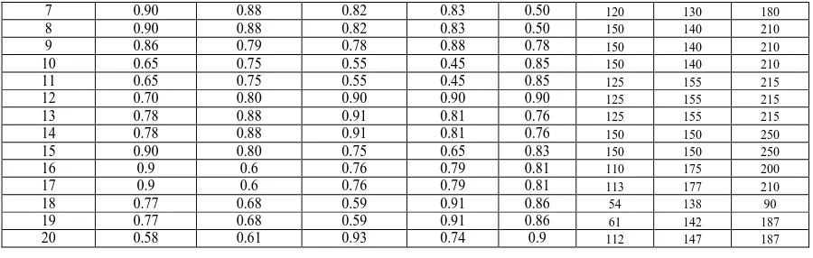
B. Twenty Different Problems

TABLE 7

Shows 20 problems containing subsystem’s reliability

Problem No. R1(x1) R2(x2) R3(x3) R4(x4) R5(x5) C1 C2 C3

1 0.80 0.85 0.90 0.65 0.75 110 175 200

2 0.70 0.90 0.55 0.65 0.85 110 175 200

3 0.90 0.95 0.55 0.85 0.55 110 175 220

4 0.80 0.70 0.60 0.80 0.70 115 140 220

5 0.60 0.78 0.65 0.82 0.70 115 140 220

(5)

IJEDR1603110

676

7 0.90 0.88 0.82 0.83 0.50 120 130 180

8 0.90 0.88 0.82 0.83 0.50 150 140 210

9 0.86 0.79 0.78 0.88 0.78 150 140 210

10 0.65 0.75 0.55 0.45 0.85 150 140 210

11 0.65 0.75 0.55 0.45 0.85 125 155 215

12 0.70 0.80 0.90 0.90 0.90 125 155 215

13 0.78 0.88 0.91 0.81 0.76 125 155 215

14 0.78 0.88 0.91 0.81 0.76 150 150 250

15 0.90 0.80 0.75 0.65 0.83 150 150 250

16 0.9 0.6 0.76 0.79 0.81 110 175 200

17 0.9 0.6 0.76 0.79 0.81 113 177 210

18 0.77 0.68 0.59 0.91 0.86 54 138 90

19 0.77 0.68 0.59 0.91 0.86 61 142 187

20 0.58 0.61 0.93 0.74 0.9 112 147 187

C. Solutions of Twenty Different Problems

TABLE 8

Shows Optimal Redundancy, system reliability and iteration.

Problem No. Redundancy

Constrains Reliability Iteration

x1,x2,x3,x4,x5 C1 C2 C3 Rs(xi) u

1 3,3,3,2,1 110 175 200 0.9993 2800 2 2,1,4,3,1 110 175 200 0.9910 1800 3 4,2,2,1,3 110 175 220 0.9996 900 4 3,2,2,2,2 115 140 220 0.9939 2500 5 3,2,3,2,1 115 140 220 0.9933 1900 6 2,2,4,2,1 120 130 180 0.9944 2600 7 1,1,2,3,3 120 130 180 0.9957 1900 8 1,3,3,2,2 150 140 210 0.9986 1100 9 2,1,3,3,1 150 140 210 0.9989 1700 10 2,4,3,1,1 150 140 210 0.9775 1600 11 2,4,3,3,1 125 155 215 0.9854 2100 12 3,2,3,2,1 125 155 215 0.9995 1200 13 3,2,2,3,3 125 155 215 0.9998 1000 14 2,3,3,3,2 150 150 250 0.9858 1300 15 3,4,3,1,1 150 150 250 0.9994 1600 16 1,2,3,3,3 110 175 200 0.9971 1100 17 3,2,3,4,1 113 177 210 0.9993 1400 18 5,2,1,2,1 54 138 90 0.9931 1700 19 4,3,1,2,2 61 142 187 0.9983 1900 20 1,3,3,4,1 112 147 187 0.9994 2400

D. Subjected to Non Linear (Non Separable) Constraints

g1(x) = 2x1x22 + 3x3x42 + 4x4x52 ≤ C1

g2(x) = 7(x1+exp(x1/4))+7(x2+exp(x2/4))+5(x3+exp(x3/4))+9(x4+exp(x4/4) ≤ C2 g3(x) = 7x1exp(x2/4) + 8x2exp(x1/4) +8x3exp(x4/4) + 6x4exp(x3/4) + 9x4exp(x5/4) ≤ C3

E. Twenty Different Problems

TABLE 9

Contains the subsystem’s reliability and consumed resources

Reliabilities Ri (xi) Constraints

Problem No. R1 R2 R3 R4 R5 C1 C2 C3

(6)

IJEDR1603110

677

18 0.77 0.68 0.59 0.91 0.86 70 145 150 19 0.77 0.68 0.59 0.91 0.86 70 138 140 20 0.58 0.61 0.93 0.74 0.90 170 160 210

F. Solution of Twenty Different Problems

TABLE 10

Shows Optimal Redundancy and system reliability and Constrains

Problem No. Redundancy Constraints Reliability Iteration

{xi} C1 C2 C3 RS(xi) u

1 1,3,4,1,3 66 126 122 0.9977 1600

2 5,2,4,1,2 68 154 186 0.9964 2600

3 3,2,2,1,2 46 115 114 0.9993 600

4 2,3,3,2,2 104 134 164 0.9961 2400

5 3,3,2,2,1 86 132 165 0.9909 2700

6 1,2,4,2,2 88 123 147 0.9913 1800

7 2,3,1,2,2 80 120 127 0.9980 2800

8 3,3,2,2,2 110 137 171 0.9999 1400

9 1,3,3,3,1 111 133 169 0.9984 1700

10 3,3,4,1,1 70 135 164 0.9863 2500

11 3,4,3,1,1 109 138 180 0.9907 2800

12 4,3,1,2,1 116 142 183 0.9991 1400

13 2,3,3,3,1 129 142 193 0.9999 1800

14 1,3,3,3,2 147 138 179 0.9997 1900

15 2,3,3,3,1 129 142 193 0.9994 2400

16 3,3,3,2,1 98 139 183 0.9970 1200

17 1,3,3,3,1 111 133 169 0.9977 2600

18 5,1,2,2,2 66 141 149 0.9963 2100

19 1,3,5,1,3 69 135 137 0.9943 2800

20 4,3,2,2,3 168 168 209 0.9992 1800

VIII.RESULTSANDCONCLUSIONS

In this paper, the Proposed Monte Carlo method is applied to different problems of bridge and complex (5 nodes,7edges) system to optimize the system reliability under the given constraints.

This leads to the conclusion that the system reliability of Monte Carlo is much more optimized and we can get better result. The proposed method is also not affected by any kind or number of constraints which is shown by applying different problems. Its simplicity and suitability for computer solution makes this method highly useful to reliability engineers. It has not been rigorously proved that this method is exact, but no faulty solution has yet been found. Even if the method is not exact, it appears to be very close and we get better optimal solution for any complex system.

REFERENCES

1. D.K. Kulshrestha, M.C. Gupta, "Use of dynamic programming for reliability engineers, IEEE Trans. Reliability, vol R-22, pp 240- 241 (Oct 1973).

2. P.J. Kolesar, "Linear programming and the reliability of multi component systems," Naval Research Logistics Quarterly, vol 15, pp 317-327 (Sep 1967).

3. K.B. Misra, "A method of solving redundancy optimization problems," IEEE Trans. Reliability, vol R-20, pp 1 17-120 (Aug 1971).

4. K.K. Aggarwal, "Redundancy optimization in general systems," IEEE Trans. Reliability, vol R-25, pp 330-332 (Dec 1976). 5. F. Altiparmak, B. Dengiz, and A. E. Smith, “Optimal design of reliable computer networks: A comparison of

metaheuristics,” J. Heuristics vol. 9, no. 6, pp. 471–487, Dec. 2003.

6. J. Y. Lin and C. E. Donaghey, “Monte Carlo simulation to determine minimal cut sets and system reliability,” in Proceedings of the 1993 Annual Reliability and Maintainability Symposium, Atlanta, GA, USA, 1993.

7. Dinghua, Shi; “A New Heuristic Algorithm for Constrained Redundancy-Optimization in Complex Systems,” IEEE Trans.Reliability, Volume: R-36, pp 621 – 623(Dec 1987)