Serial and Parallel Iterative Splitting Methods:
Algorithms and Applications
J¨
urgen Geiser
a, Jose L. Hueso
b, Eulalia Mart´ınez
baDept. of Electrical Engineering and Information Technology, Ruhr-University of Bochum, Germany bInstituto Universitario de Matem´atica Multidisciplinar. Universitat Polit`ecnica de Val`encia, Spain
Abstract
The properties of iterative splitting methods with serial versions have been analyzed since recent years, see [1] and [3]. We extend the iterative splitting methods to a class of parallel versions, which allow to reduce the computational time and keep the benefit of the higher accuracy with each iterative step. Parallel splitting methods are nowadays important to solve large problems, which can be splitted in subproblems and computed independently with the different processors. We present a novel parallel iterative splitting method, which is based on the multi-splitting methods, see [2], [10] and [15]. Such a flexibilisation with multisplitting methods allow to decompose large iterative splitting methods and recover the benefit of their underlying waveform-relaxation (WR) methods. We discuss the convergence results of the parallel iterative splitting methods, while we could reformulate such an error to a summation of the individual WR methods. We discuss the numerical convergence of the serial and parallel iterative splitting methods and present different numerical applications to validate the benefit of the parallel versions.
Key words: Multisplitting method; iterative splitting method; numerical analysis; operator-splitting method; initial value problem; iterative solver method; Waveform relaxation method.
AMS subject classifications:35K45, 35K90, 47D60, 65M06, 65M55.
1. Introduction
Iterative splitting methods are nowadays important solver methods to solve large systems of ordinary, partial or stochastic differential equations, see [1], [3] and [7]. Iterative splitting methods are based on two solver ideas, while in the first part we separate the full operators into different sub-operators and reduce the computational time for such sub-computation, an additional benefit is the iterative part, which allows to solve a relaxation problem, like known in waveform-relaxation method or Picard’s iterative method, see [6], [11] [12] and [13]. Both parts reduce the computational time and the complexity as if we solve all parts (full operator and direct method) together, see [5]. Such iterative splitting methods can be used to solve with less computational amount an approximate solution of the ordinary differential equations (ODEs) or semi-discretized partial differential equations (PDEs), see [5] and [13]. The bottleneck of all the iterative methods are given by the large sizes of the iterative matrices, see [10] and [15], therefore we
considered parallel versions of the iterative splitting method, see [2] and [4]. We concentrate on solving linear evolution equations, such as the differential equation,
∂tc=Ac= L
X
l=1
Alc, c(0) =c0, (1)
whereA∈IRm×IRm is the full operator withm is the finite dimension of the operator andA
l are
sub-operators. Furtherc ∈C1([0, T]; IRm) is the solution andc
0 ∈IRm is the initial condition. Based on the decomposition of the large scale differential equation with operatorAinto different smaller sub-differential equations with operators Al, where l = 1, . . . , L and L is the number of processors, we distribute the
computational time to many processors and reduce the computational time, see [15]. Further, we modify the synchronous parallel splitting method with chaotic (asynchronous) ideas, such that the computation and communication of the various processors can be done completely independently, see [14].
The outline of this paper is as follows. The serial iterative splitting method is explained in Section 2. The parallel iterative splitting method is introduced in Section 3. We discuss the theoretical results in Section 4. The numerical examples are presented in Section 5. In Section 6, we discuss the theoretical and practical results.
2. Serial iterative splitting method
We consider a two-level iterative splitting method, which is discussed for two operators in [3] and for L-operators in [8].
Based on the differential equation (1), we have the following decomposition of the operatorA: – A=PL
l=1Al , whileAl are the sub-operators for the iterative part (solver part),
– andBl=A−Alare the sub-operators for the relaxation part (right hand side part).
where we havel= 1, . . . , L.
The serial iterative splitting method is given in the following algorithm. Here, we apply a fixed-splitting discretization step-size τ, namely, on the time-interval [tn, tn+1]. We solve the following sub-problems consecutively fori= 0, L, . . . ,(m−1)L:
∂ci+1(t)
∂t =A1ci+1(t) + B1ci(t), with ci+1(t
n) =cn, (2)
∂ci+2(t)
∂t =A2ci+2(t) + B2ci+1(t), with ci+2(t
n) =cn, (3)
. . . (4)
∂ci+L(t)
∂t =ALci+L(t) + BLci+L−1(t), with ci+L(t
n) =cn, (5)
where we assume for the first initialisation c0(t) = 0.0, further cn is the known split approximation
at the time-level t = tn. The split approximation at the time-level t = tn+1 is defined as cn+1 = c(m−1)L(tn+1). The stopping criterion is ||c(m−1)L −c(m−2)L|| ≤ err and then we have the solution c(tn+1) =c(m−1)L(tn+1).
The solutions are given as:
ci+1(t) = exp(A1(t−tn))cn+
Z t
tn
exp(A1(t−s))B1ci(s)ds, (6)
ci+2(t) = exp(A2(t−tn))cn+
Z t
tn
exp(A2(t−s))B2ci+1(s)ds, (7)
. . . , (8)
ci+L(t) = exp(AL(t−tn))cn+
Z t
tn
exp(AL(t−s))BLci+L−1(s)ds, (9)
wheret∈[tn, tn+1].
We define the error-function as ei(t) = c(t)−ci(t) with e0(t) = c(t)−c0 and the maximum-norm
||ei||= maxt∈[0,T]||ei(t)||∞and the maximum operator norm||Al||=||Al||∞.
Theorem 2.1 We have bounded operatorsAl∈IRm×IRm. Then the iterations (2)-(5), which are applied
with i= 0, L, . . . ,(m−1)L, withL are the number of operators, for the Cauchy-problem (1) is of order O(τmL).
Proof 2.2 The proof is done for the 2-level method in the paper [8]. We apply a recursive argument of the iterative scheme with theL operators and obtain:
||emL|| ≤ ΠLl=1Cl||Bl||
m
||e0||, (10)
whereCl is given withCl=O(τ), see also [8].
In the following, we concentrate extend the two-level iterative splitting method to a parallel iterative splitting method, while we could transform the two-level method with multisplitting method.
3. Parallel iterative splitting method
In the following, we parallelise the serial iterative splitting approach with the idea of multisplitting-approaches.
We present in the following approaches: – Multi-splitting iterative approach,
– Two operator iterative splitting approach.
3.1. Multi-splitting iterative approach
The problem is given as ∂c∂t =Ac(t) =PL
l=1Alc(t), c=c0.
The idea is amultipledecomposition of
A=Al+Bl, l= 1, . . . , L, (11)
Bl=A−Al, (12)
whereAl is a non-singular andBl is the rest matrix.
Further, we have the decomposition of the parallel computable vectors:
ci= L
X
l=1
Elci,l, andE= L
X
l=1
El, (13)
where ci is the i-th iterative solution and ci,l are the parallel computable solutions in the i-th iterative
step.E is the identity matrix andEl are diagonal matrices with positive entries.
The multisplitting iterative approach is given as:
∂ci,l(t)
∂t =Alci,l(t) + Blci−1(t), fort∈[t
n, tn+1] (14)
with ci,l(tn) =c(tn), l= 1, . . . L,
where the initalisation is c0(t) = c(tn), we have i = 1, . . . , I iterative steps. The stopping criterion is
||ci−ci−1|| ≤errand then we have the solutionc(tn+1) =ci(tn+1).
The splitting error of the iterative splitting is ofk+ 1 order, i.e.O(τk+1), with
||erri+1||=Kiτni||err0||+O(τni+1), (15)
where Ki = P L l=1
1
ωl ||Bl|| and
PL
l=1 1
ωl = 1 are the weights (ωl > 1) and ||err0|| = ||c0(t)||, while c−1(t) = 0.
Benefit:
– Good error balance between the different operators Drawback:
– Balances in the decomposition ofElimportant to damp large errors
3.2. Parallel splitting with two operators: Classical version
We have to apply the following algorithm, which is applied with synchronisation:
∂ci,1(t)
∂t =Aci,1(t) + Bci−1(t), with ci,1(t
n) =cn, c
0= 0.0,
∂ci,2(t)
∂t =Bci,2(t) + Aci−1(t), with ci,2(t
n) =cn, c
0= 0.0,
ci(t) =
1
2(ci,1(t) +ci,2(t)), (16)
where cn is the known split approximation at the time-level t = tn. The split approximation at the
time-levelt=tn+1 is defined ascn+1=c
i(tn+1). We have the stopping criterion ||ci−ci−1|| ≤err. The solutions are given as:
ci,1(t) = exp(A(t−tn))cn+
Z t
tn
exp(A(t−s))B ci−1(s)ds, (17)
ci,2(t) = exp(B(t−tn))cn+
Z t
tn
exp(B (t−s))A ci−1(s)ds, (18)
ci(t) =
1
2(ci,1(t) +ci,2(t)), (19)
wheret∈[tn, tn+1].
The integrals can be solved by higher order integration-rules, e.g., with the Trapezoidal- or Simpson’s-rule.
3.3. Parallel splitting with two operators: Modern version
We have the following algorithm, which is applied without synchronization:
∂ci,1(t)
∂t =Aci,1(t) + Bci−1,1(t), with ci,1(t
n) =cn, c
0,1= 0.0,
∂ci,2(t)
∂t =Bci,2(t) + Aci−1,2(t), with ci,2(t
n) =cn, c
0,2= 0.0,
wherecn is the known split approximation at the time-levelt=tn.
Processorl, l= 1,2 runs the iterations independently until the stopping criterion||ci,l−ci−1,l|| ≤err
is reached . Then, the approximations are synchronized
ci(t) =
1
2(ci1,1(t) +ci2,2(t)), where processorlstops at iteration il.
The split approximation at the time-levelt=tn+1 is defined ascn+1=ci(tn+1).
4. Theoretical Results
In the following, we deal with the m-dimensional initial value problem in the non-homogeneous form, see also the homogeneous form in Equation (1):
c0(t) =Ac(t) +f(t), x(0) =x0, (20)
Further, we deal in the following with the proof-ideas related to Waveform relaxation methods, see [9] and [14].
The initial value problem (20) is solved with the multisplitting Waveform-relaxation method, which is given as:
c0i+1(t) =M ci+1(t) +N ci(t) +f(t), c(0) =c0, (21)
whereAis given in Equation (1). Furtherc0(t) =c0is the starting condition. For the multisplitting approach, we have the following Definition 4.1.
Definition 4.1 We have L≥1 is the number of the splittings. Further, we haveA, Al, Bl, El, which are
real-valuedm×m matrices. Such that we obtain the multisplitting triple(Al, Bl, El)forl= 1, . . . , L:
– A=Al+Bl andBl=P L
k=1,k6=lAk with l= 1, . . . , L,
– The matricesEl are nonnegative diagonal matrices and satisfy:P L
l=1El=I ,
whereI is the identity matrix.
– sl(i+ 1)≤i+ 1 indicates the iteration, where thel-th component is computed prior to i+ 1.
– The multisplitting approach based on the Waveform-relaxation in the classical version is given in the following notation:
c0l,i+1(t) =Alcl,i+1(t) +Blci+f(t), cl,i+1(0) =c0, (22)
ci+1(t) = L
X
l=1
Elcl,i+1(t). (23)
– The multisplitting approach based on the Waveform-relaxation in the modern version is given in the following notation:
c0s
l(i+1)(t) =Alcsl(i+1)(t) +Blci+f(t), csl(i+1)(0) =c0, (24)
ci+1(t) =
L
X
l=1
Elcsl(i+1)(t). (25)
4.1. Convergence Analysis
The solution of the multisplitting Waveform-relaxation method (22) and (23), is given as following: We solve the individual equations (22) as: can be written as:
cl,i+1(t) =Klci(t) +φl(t), (26)
where we have
Klc(t) =
Z t
0
kl(t−s)c(s)ds, forl= 1, . . . , L, (27)
φl(t) = exp(tAl)c0+
Z t
0
exp((t−s)Al)f(s)ds, forl= 1, . . . , L. (28)
wherekl(t) = exp(tAl)Blforl= 1, . . . , L.
Further, we apply the multisplitting notation (23) and obtain the summations:
Kc(t) =
L
X
l=1
ElKlc(t), (29)
φ(t) =
L
X
l=1
Elφl(t), (30)
wherek(t) =PL
ci+1(t) =Kci(t) +φ(t). (31)
We assume, that the Lemma 4.2 is fulfilled, see also [9].
Lemma 4.2 We assume that the following items are equivalent: – We assume c(t) is a solution of the initial value problem (20).
– c(t)is a solution of each multisplitted equationc(t) =Klc(t) +φl(t), c(0) =c0, l= 1, . . . , L.
– c(t)is the solution of the fixpoint equation c(t) =Kc(t) +φl(t).
We define||c||T = maxt∈[0,T]|c(t)|as maximum norm and we also us|| · ||as a matrix norm induced by the vector norm| · |.
Based on the assumptions, we derive in the following the errors and the convergence results.
In the Theorem 4.3 we derive the error of thei-th approximation, see also [9].
Theorem 4.3 There exists a constant C := PL
l=1Cl, which is given to estimate the kernel k of the
multisplitting waveform-relaxation operator, such that we obtain ||k||T = C. Then the error of the i-th
approximation of the classical multisplitting WR method (22)-(23) is given by
||ci−c||T ≤
(CT)i
i! (exp(CT)||φ||T +||c0||T). (32)
Proof 4.4 We have given
ci(t) =Kci−1(t) +φ(t), (33)
We apply the Lemma 4.2 and follow with the iterative approach:
ci(t) =Kic0(t) + i−1
X
j=0
Kiφ(t), (34)
where isKiu(t)is thei-times convolution
Kiu(t) =Rt
0k(t−si)(
Rsi
0 k(t−si−si−1)(. . .
Rt− Pi
j=0si−j 0 k(t−
Pi
j=0si−j)u(s1)ds1. . .)dsi−1)dsi.
Further we have ||u||T = maxt∈[0,t]|u(t)|, where| · | is an appropriate Banach-Norm.
It exists:
||kl||T ≤Cl, forl= 1, . . . , L, (35)
and we have
|k(t)| ≤ ||k||T =|| L
X
l=1
Elkl|| ≤ L
X
l=1
Cl=C, (36)
we apply the estimation of the Waveform-relaxation, see [11], and obtain:
||Ki||T ≤
(CT)i
i! , (37)
where we have limi→∞||Ki||T →0.
The error estimate is than given as
||c−ci||T =||( lim j→∞K
jc
0−
∞
X
j=0
Kjφ(t))−(Kic0−
i−1
X
j=0
Kjφ(t))||
≤ ||
∞
X
j=i
Kjφ(t) +Kic0|| ≤ ||Ki||T(||
∞
X
j=0
Kj||φ(t)||T +||c0||T). (38)
∞
X
j=0
Kj=K0+K1+. . .+K∞≤exp(CT). (39)
Then we obtain the estimation
||c−ci||T =≤
(CT)i
i! (exp(CT)||φ||T +||c0||T). (40)
We have the following new convergence Theorem 4.5 based on the extension of the classical convergence Theorem version 4.3.
Theorem 4.5 There exists a constant C := PL
l=1Cl, which is given to estimate the kernel k of the
multisplitting waveform-relaxation operator, such that we obtain ||k||T =C. Then the convergence of the
modern multisplittting WR method (24)-(25) is given by
||cimin−c|| T ≤
(C T)imin imin! ||c
0−c||
T, (41)
whereimin= minLl=1sl(i), wheresl(i)≤iare the retarded iterations of the l-th processor. Proof 4.6 We start with the estimation of the i-th iteration:
||cimin−c|| T ≤ ||
X
l=1
ElKl(csl(i)−c)||T ≤ (42)
≤ ||X
l=1
ElKl(cimin−1−c)||T ≤ ||K||T ||(cimin−1−c)||T. (43)
Then, we have the recursion:
||cimin−c||
T ≤ ||Kimin||T||(c0−c)||T. (44)
where we apply ||Kimin||
T ≤ (C T) imin
imin! , based on the idea in [11], and we obtain:
||cimin−c|| T ≤
(C T)imin imin!
||(c0−c)||T, (45)
whereimin= minLl=1sl(i).
Remark 4.7 For the parallel error, we have the order O(τm), if we assume that all processors have at
leastmiterative cycles, while for the serial error, we have the orderO(τmL). Means in the serial version,
we have to apply mL iterative steps in sum to obtain the result, while in the parallel version, we only apply m iterative steps, while L processors share the computation to solve the L sub-equations. Further, we can assume, that the sub-equations are faster to solve, while the sub-operators are much more smaller and simpler to handle. Such that we have tsub≤
tf ull
L , while tsub is the time to solve a sub-problem and tf ull the time to solve the full problem. Therefore, we have a benefit in the parallel distribution and we
obtain faster the higher order O(τmL)as with the serial version.
Remark 4.8 We can modify the parallel method with inner and outer iterative cycles. Means we deal withL inner cycles for each processor and applym outer cycles for all the processors. For such methods, we also obtain the higher order O(τmL) but more faster than in the serial version.
5. Numerical examples
In the following, we deal with different numerical example to verify and test the theoretical results. We deal with:
– Only time-dependent problem: We apply ordinary differential equation to verify the theoretical results. – Linear time and spatial dependent problem: We apply a diffusion equation with different spatial
depen-dent operators and test the application to partial differential equations.
5.1. First Example: Matrix problem
For a first test example, consider the matrix equation,
u0(t) =
1 2
0 1
u, u(0) =u0=
1
1
, (46)
the exact solution is
exp( 1 2 0 1 t) =
exp(t) 2t exp(t)
0 exp(t)
. (47)
We split the matrix as, – Two operator approach
A+B=
1 2 0 1 =
0.3 1
0 0.3
+
0.7 1
0 0.7
(48)
– Multiple operator approach
A1+B1=
1 2 0 1 =
0.1 1.0
0 0.1
+
0.9 1.0
0 0.9
(49)
A2+B2=
1 2 0 1 =
0.5 0.1
0 0.5
+
0.5 1.9
0 0.5
(50)
where theE1 andE2are given as:
E1=
0.9 0
0 0.1
, E2=
0.1 0
0 0.9
. (51)
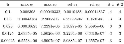
We include Tables 1 and 2 corresponding to Multi-splitting iterative approach classical and modern version with the above partitions and using different discretizations in [0,1] of stephallowing a maximum of 10 iterations and a tolerance of 10−3.We can see in the results the relative and absolute errors for each component of the solution and the mean of iterations performed in order to reach the tolerance.
h maxe1 maxe2 rele1 rele2 it 1 it 2 0.1 0.008308 0.00040332 0.0010188 0.00014837 4 4 0.05 0.00043184 2.906e-05 5.2955e-05 1.069e-05 3 3 0.025 0.00010623 7.2291e-06 1.3027e-05 2.6595e-06 3 3 0.0125 2.6335e-05 1.8026e-06 3.2294e-06 6.6316e-07 3 3 0.00625 6.5553e-06 4.5007e-07 8.0385e-07 1.6557e-07 3 3 Table 1
Multisplitting classic version
h maxe1 maxe2 rele1 rele2 it 1 it 2 0.1 0.0081586 0.0003996 0.0010005 0.000147 4 4 0.05 0.00030027 3.1292e-05 0.00012447 1.1512e-05 3.35 3 0.025 0.00027348 1.3123e-05 3.3536e-05 4.8277e-06 3 3 0.0125 6.8274e-05 3.281e-06 8.3723e-06 1.207e-06 3 3 0.00625 1.7056e-05 8.2026e-07 2.0915e-06 3.0176e-07 3 3 Table 2
Multisplitting Modern version
5.2. Second Example: Diffusion problem
We deal with the following diffusion problem:
u0(x, t) = ∆u(x, t), (x, t)∈∂Ω×[0, T], (52)
u(x,0) = sinx siny sinz, x∈Ω, (53)
u(x, t) = 0, (x, t)∈∂Ω×[0, T], (54)
where we have the analytical solution uan(x, t) = exp(−3t) sinx siny sinz, with x = (x, y, z)t and
Ω = [−π, π]×[−π, π]×[−π, π].
In operator notation, we write as following:
A=A1+A2+A3, (55)
where A1 = ∂ 2
∂x2, A2 = ∂ 2
∂y2, A3u = ∂ 2
∂z2 and we assume, that the zero-boundary conditions (Dirichlet boundary conditions) are embedded.
The problem is discretized by using a 4-D mesh in Ω×[0, T]. Denote byui,j,k,tthe approximated value of
the solution at node (xi, yj, zk, t) for a givent. For the time-integration, we apply the integral formulation,
see Equations (6)-(9).
For the spatial discretization, we test a second and fourth order scheme:
∂2
∂x2ui,j,k,t=
ui+1,j,k,t−2ui,j,k,t+ui−1,j,k,t
∆x2 , second order approach, (56)
∂2
∂x2ui,j,k,t=
−ui+2,j,k,t+ 16ui+1,j,k,t−30ui,j,k,t+ 16ui−1,j,k,t−ui−2,j,k,t
12∆x2 , 4th-order approach, (57)
where we have the analogous operators for they andz derivations.
In order to establish the convergence of the algorithms, we compute the solutionu(∆x, h) obtained using spatial and temporal steps ∆x= ∆y= ∆zandh,respectively. We use different measures to estimate the convergence. On one hand, we can compare the outcome of the methodu(∆x, h) with the exact solution uana for every point of the mesh, which shows the convergence of the method. On the other hand, we
can compare u(∆x, h) with the result obtained halving the time or space steps, h/2 or ∆x/2, at the points shared by the corresponding meshes. This allows to analyze how the results depend on these steps. Denote byei,j,k(∆x, h) the difference between the results at a mesh point (xi, yj, zk, T), obtained using
two different time or space steps, and by δi,j,k(∆x, h) the difference with the analytical solution at the
same point. In the tables, we will denote the maximum errors by
emax= max
i,j,k |ei,j,k(∆x, h)|, (58)
and
δmax= max
i,j,k |δi,j,k(∆x, h)|, (59)
and the mean errors by
emean= 1 N
X
i,j,k
and
δmean= 1 N
X
i,j,k
|δi,j,k(∆x, h)|, (61)
whereN is the number of spatial nodes at timeT.
In the following, we discuss different decompositions of the multi-operator splitting approach: – Directional decomposition: We decompose into the different directions:
A1= ∂2
∂x2, A2= ∂2
∂y2, A3= ∂2
∂z2. (62)
Here, we have the benefit of decomposing the different directions.
The drawback is related to the unbalanced decomposition, while the matrices have different sparse entries. Therefore the exponential matrices of the operators are different in their sparse behaviour and the error can not be optimal reduced.
We can reduce the unbalanced problem, if we deal with the idea to use ∆t≈∆x, see [8]. Then, we obtain at least a second order scheme (related to the spatial discretization).
At least, we test also the strong relation of the time- and spatial scales with respect to the explicit CFL condition, means, we have:
∆t≈ ∆x
2
6 , (63)
where ∆x= ∆y= ∆z.
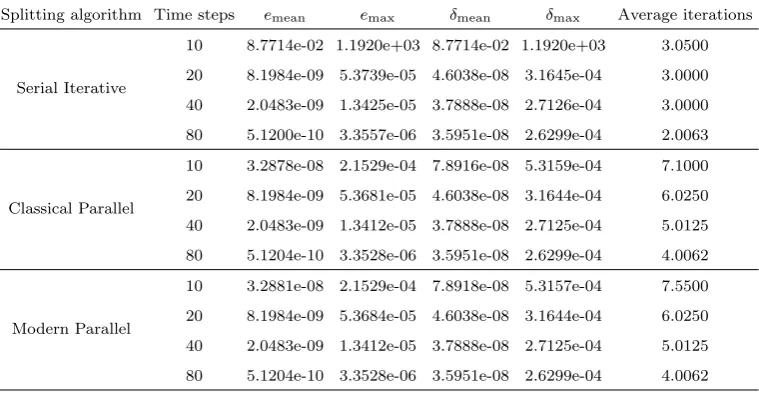
We apply the splitting algorithms with the directional decomposition in [0,1]. The splitting is iterated until a tolerance of 10−8 or a maximum of 10 iterations are reached. The values shown in the tables correspond to maximum or mean values at T = 1. Tables 3 and 4 present the results obtained using different number of temporal steps and the second and fourth order schemes for the spatial discretization, respectively. In tables 5 and 6, we fix the number of temporal steps to 1280 and vary the number of spatial intervals.
Splitting algorithm Time steps emean emax δmean δmax Average iterations
Serial Iterative
10 3.0021e-05 8.8220e-03 1.3021e-04 2.0943e-02 4.0000 20 1.6139e-05 4.7546e-03 1.1744e-04 2.0304e-02 3.0000 40 7.8770e-06 2.2831e-03 1.1352e-04 2.0135e-02 3.0000 80 3.8391e-06 1.1013e-03 1.1245e-04 2.0059e-02 2.0688
Classical Parallel
10 7.5244e-06 1.1242e-03 1.1498e-04 2.0319e-02 9.9500 20 4.1720e-06 6.1563e-04 1.2189e-04 2.0942e-02 7.0000 40 2.1715e-06 3.1759e-04 1.2579e-04 2.1295e-02 5.0750 80 1.1042e-06 1.6070e-04 1.2784e-04 2.1479e-02 4.8688
Modern Parallel
10 6.9978e-06 8.6818e-04 1.1445e-04 1.9636e-02 9.9000 20 4.2214e-06 5.4241e-04 1.2128e-04 2.0487e-02 7.9750 40 2.3180e-06 3.0696e-04 1.2536e-04 2.1029e-02 6.0000 80 1.2147e-06 1.6316e-04 1.2758e-04 2.1336e-02 4.9938 Table 3
Results using the second order scheme for the spatial discretization, with 10 spatial subintervals and different number of temporal steps
Splitting algorithm Time steps emean emax δmean δmax Average iterations
Serial Iterative
10 8.7714e-02 1.1920e+03 8.7714e-02 1.1920e+03 3.0500 20 8.1984e-09 5.3739e-05 4.6038e-08 3.1645e-04 3.0000 40 2.0483e-09 1.3425e-05 3.7888e-08 2.7126e-04 3.0000 80 5.1200e-10 3.3557e-06 3.5951e-08 2.6299e-04 2.0063
Classical Parallel
10 3.2878e-08 2.1529e-04 7.8916e-08 5.3159e-04 7.1000 20 8.1984e-09 5.3681e-05 4.6038e-08 3.1644e-04 6.0250 40 2.0483e-09 1.3412e-05 3.7888e-08 2.7125e-04 5.0125 80 5.1204e-10 3.3528e-06 3.5951e-08 2.6299e-04 4.0062
Modern Parallel
10 3.2881e-08 2.1529e-04 7.8918e-08 5.3157e-04 7.5500 20 8.1984e-09 5.3684e-05 4.6038e-08 3.1644e-04 6.0250 40 2.0483e-09 1.3412e-05 3.7888e-08 2.7125e-04 5.0125 80 5.1204e-10 3.3528e-06 3.5951e-08 2.6299e-04 4.0062 Table 4
Results using the fourth order scheme for the spatial discretization, with 10 subintervals in each dimension and different number of temporal steps
Table 4 shows that, using the fourth order scheme, the order of convergence of with respect to the temporal stephis 2, being the estimated errors proportional toh2.
Splitting algorithm Space intervals emean emax δmean δmax Average iterations 10 6.0092e-05 1.0185e-02 1.1203e-04 2.0006e-02 2.0031 Serial Iterative 20 2.7133e-05 4.9543e-03 5.3066e-05 9.8264e-03 2.0219
40 − − 2.6073e-05 4.8721e-03 3.0000
10 5.9473e-05 9.5024e-03 1.2940e-04 2.1621e-02 4.0031 Classical parallel 20 3.4999e-05 5.9655e-03 7.0607e-05 1.2119e-02 4.2938
40 − − 3.5660e-05 6.1534e-03 6.0219
10 5.9809e-05 9.5336e-03 1.2933e-04 2.1583e-02 4.0031 Modern Parallel 20 3.5212e-05 6.0031e-03 7.0192e-05 1.2050e-02 5.9781
40 − − 3.5029e-05 6.0466e-03 9.9812
Table 5
Results using the second order scheme for the spatial discretization, with 320 temporal steps and different number of spatial subintervals
In Table 5, the spatial step is reduced simultaneously in the three dimensions, in order to keep the increments equal, because the performance of the method is better in this case. The number of time steps is big enough to ensure the convergence in the case of smaller spatial subinterval and is used in all the cases to allow the comparison depending only on the spatial step. The error is halved when the step in each spatial dimension is halved, which increases the computational cost by a factor of 8, thus the behavior of the method is poor. The parallel methods obtain slightly less approximation to the analytical result and require more iterations than the serial iterative method. The modern parallel method needs more iterations per step to converge than the classical parallel method.
Table 6 compares the results obtained varying the number of spatial subintervals. The error is divided by about 20 when the step in each spatial dimension is halved, which indicates a convergence of order higher than linear with respect to the cube of the spatial step, improving the behavior of the method with respect to the order two scheme. There is no noticeable difference in the results among the different methods, although the parallel ones require double number of iterations than the sequential method to converge.
Splitting algorithm Space intervals emean emax δmean δmax Average iterations 1 10 3.3808e-08 2.4779e-04 3.5363e-08 2.6041e-04 2.0031 1 20 1.5518e-09 1.2258e-05 1.5936e-09 1.2625e-05 2.0031
1 40 − − 4.5839e-11 3.6643e-07 2.0031
2 10 3.3808e-08 2.4779e-04 3.5363e-08 2.6041e-04 4.0031 2 20 1.5518e-09 1.2258e-05 1.5936e-09 1.2625e-05 4.0031
2 40 − − 4.5838e-11 3.6642e-07 4.0031
3 10 3.3808e-08 2.4779e-04 3.5363e-08 2.6041e-04 4.0031 3 20 1.5518e-09 1.2258e-05 1.5936e-09 1.2625e-05 4.0031
3 40 − − 4.5838e-11 3.6642e-07 4.0031
Table 6
Results using the fourth order scheme for the spatial discretization, with 320 temporal steps and different number of subin-tervals in each dimension
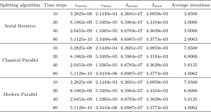
A1= 1
3A, A2= 1
3A, A3= 1
3A. (64)
Here, we have the benefit of equal load balances of the matrices, such that the exp-matrices have the same sparse structure.
Splitting algorithm Time steps emean emax δmean δmax Average iterations
Serial Iterative
10 3.2825e-08 2.1449e-04 6.2681e-07 4.0959e-03 3.0500 20 8.1862e-09 5.3493e-05 6.5964e-07 4.3104e-03 3.0000 40 2.0453e-09 1.3365e-05 6.6783e-07 4.3639e-03 3.0000 80 5.1125e-10 3.3408e-06 6.6987e-07 4.3773e-03 2.0063
Classical Parallel
10 3.2825e-08 2.1449e-04 6.2681e-07 4.0959e-03 7.0500 20 8.1862e-09 5.3493e-05 6.5964e-07 4.3104e-03 6.0000 40 2.0453e-09 1.3365e-05 6.6783e-07 4.3639e-03 5.0125 80 5.1128e-10 3.3410e-06 6.6987e-07 4.3773e-03 4.0062
Modern Parallel
10 3.2825e-08 2.1449e-04 6.2681e-07 4.0959e-03 7.0500 20 8.1862e-09 5.3493e-05 6.5964e-07 4.3104e-03 6.0000 40 2.0453e-09 1.3365e-05 6.6783e-07 4.3639e-03 5.0125 80 5.1128e-10 3.3410e-06 6.6987e-07 4.3773e-03 4.0062 Table 7
Results using the second order scheme for the spatial discretization, with 10 spatial subintervals and different number of temporal steps
– Mixed decomposition: We decompose into the different directions:
A1= (1−) ∂2 ∂x2 +
2(
∂2 ∂y2 +
∂2
∂z2), A2= (1−) ∂2 ∂y2 +
2(
∂2 ∂x2 +
∂2
∂z2), (65)
A3= (1−) ∂2 ∂z2 +
2(
∂2 ∂x2 +
∂2
∂y2), (66)
where = [0,2/3], means for = 0, we have the directional decomposition, while for= 2/3 we have the balanced decomposition.
Here, we have the benefit, e.g., for small= 0.1, we have nearly a directional decomposition scheme. Based on the6= 0, we stabilise the scheme.
Remark 5.3 We obtain the benefit of the classical and modern parallel iterative splitting method based on larger time-steps and more iterative steps. In such an optimal version, we are much faster than the serial version and also the result is more accurate. For very fine time-steps, we do not see an improvement in the accuracy, but we see a benefit in the computational time, means the parallel versions are more faster.
5.3. Third Example: Mixed convection-diffusion and Burgers equation
We deal with a partial differential equation, which is a 2D example of a mixed convection-diffusion and Burgers equation. For such equations, we can find analytical solution. The model problem is given as:
∂tu=−1/2u∂xu−1/2u∂yu−1/2∂xu−1/2∂yu
+µ(∂xxu+∂yyu) +f(x, y, t), (x, y, t)∈Ω×[0, T], (67)
u(x, y,0) =uana(x, y,0), (x, y)∈Ω, (68)
u(x, y, t) =uana(x, y, t) on∂Ω×[0, T], (69)
where Ω = [0,1]×[0,1],T = 1.25, and µis the viscosity. The analytical solution is given as
uana(x, y, t) = (1 + exp(
x+y−t 2µ ))
−1+ exp(x+y−t
2µ ), (70)
where we computef(x, y, t) accordingly.
As in the previous example, denote byu(∆, h) the numerical solution obtained using spatial subintervals of amplitude ∆ = ∆x = ∆y, time steps h and a tolerance of tol = 10−6, allowing a maximum of 40 iterations. On one hand, we will compare the numerical solution with the exact oneuana for every point
of the mesh, which shows the convergence of the method. On the other hand, we will compare u(∆, h) with the result obtained halving the time steps, h/2, at the points shared by the corresponding meshes. Denote by ei,j,k(∆, h) the difference between the results obtained using two different time steps, h and h/2, at a common mesh point (xi, yj, tk), and byδi,j,k(∆, h) the difference with the analytical solution at
the same point. In the tables, we will use the error estimates given by
emax= max
i,j,k |ei,j,k(∆, h)|, (71)
and
δmax= max
i,j,k |δi,j,k(∆, h)|, (72)
and the mean errors by
emean= 1 N
X
i,j,k
|ei,j,k(∆, h)|, (73)
and
δmean= 1 N
X
i,j,k
|δi,j,k(∆, h)|, (74)
whereN is the total number of nodes (xi, yj, tk).
In order to obtain the temporal cost of the parallel schemes, we measure the time consumed by processor lin each iterationm, in [tk, tk+1],tpk,l,m. In the classical parallel scheme the processors synchronize at each
iteration, so the cost for this time interval istpk=Pmmax
l=1,2tpk,l,m, whereas, in the modern parallel scheme, the processors iterate independently in [tk, tk+1] performingml, l= 1,2 iterations until convergence, thus,
the cost istpk = max l=1,2
P
m tpk,l,m. The final cost is obtained adding the results of all time subintervals.
The values have been obtained using etime, running Matlab 2015a on a desktop computer with an Intel Core i7 processor in a 64 bits operating system with Windows 7 Professional.
A(u)u=−1/2u∂xu−1/2∂xu+µ∂xxu, (75)
B(u)u=−1/2u∂yu−1/2∂yu+µ∂yyu+f(x, y, t). (76)
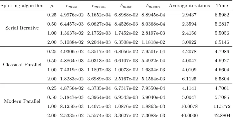
Before studying the convergence of the method, we analyze the influence of parameterµ. Tables 9 and 8 compare the results obtained for different values of µ using the second and the fourth order discretization scheme, respectively, taking 10 subintervals in each spatial dimension and 640 time steps. As we can observe, the error generally increases with µ. Along this example, we will take µ = 0.5, because for this value, the methods require the minimum number of iterations, except in one case.
Splitting algorithm µ emax emean δmax δmean Average iterations Time
Generalized Iterative
0.25 4.3464e-02 5.3355e-04 2.2106e-01 8.4732e-03 2.9719 6.1689 0.50 5.1944e-03 5.5729e-04 6.0042e-03 9.4742e-04 2.5703 5.4561 1.00 1.3508e-02 2.0793e-03 1.7504e-02 2.7070e-03 2.7891 5.9197 2.00 4.9564e-02 8.9366e-03 6.2889e-02 1.1465e-02 3.0187 6.5253
Classical Parallel
0.25 1.6915e-02 3.7593e-04 2.2038e-01 8.4779e-03 4.1391 4.4844 0.50 4.0117e-03 4.0302e-04 4.6768e-03 7.1258e-04 4.0047 4.8457 1.00 8.2553e-03 1.2533e-03 1.1192e-02 1.7195e-03 4.0094 4.3426 2.00 2.1603e-02 3.9868e-03 2.9915e-02 5.5900e-03 5.0422 5.5451
Modern Parallel
0.25 1.7583e-02 3.7876e-04 2.1864e-01 8.4754e-03 4.1578 4.4456 0.50 4.2148e-03 4.3094e-04 4.9121e-03 7.4444e-04 4.0062 4.3670 1.00 9.0609e-03 1.4340e-03 1.2127e-02 1.9278e-03 8.0031 8.6506 2.00 2.5669e-02 5.1563e-03 3.4678e-02 6.9560e-03 30.0156 33.3511 Table 8
Results of the directional decomposition using the second order scheme for the spatial discretization, with 10 spatial subin-tervals, 640 temporal intervals and different values ofµ.
Splitting algorithm µ emax emean δmax δmean Average iterations Time
Serial Iterative
0.25 4.9976e-02 5.1652e-04 6.8988e-02 8.8945e-04 2.9437 6.5982 0.50 6.4457e-03 6.0827e-04 8.4526e-03 8.0368e-04 2.3594 5.2817 1.00 1.3637e-02 2.1752e-03 1.7452e-02 2.8197e-03 2.4156 5.5056 2.00 5.1088e-02 9.2044e-03 6.3508e-02 1.1818e-02 3.0922 6.5146
Classical Parallel
0.25 4.9306e-02 4.3517e-04 6.8056e-02 7.9501e-04 4.2078 4.7986 0.50 4.8864e-03 4.0313e-04 6.6107e-03 5.4922e-04 4.0047 4.5927 1.00 7.4319e-03 1.1897e-03 1.0073e-02 1.6334e-03 4.0109 4.6604 2.00 1.8283e-02 3.6989e-03 2.5167e-02 5.1564e-03 6.1125 6.5804
Modern Parallel
0.25 4.8756e-02 4.3735e-04 6.7317e-02 7.9550e-04 4.1141 4.7061 0.50 5.1847e-03 4.3964e-04 6.9543e-03 5.9040e-04 5.0047 5.7085 1.00 8.1250e-03 1.4075e-03 1.0876e-02 1.8863e-03 10.0078 11.5772 2.00 2.5335e-02 5.5574e-03 3.3627e-02 7.3088e-03 40.0000 42.8804 Table 9
Results of the directional decomposition using the fourth order scheme for the spatial discretization, with 10 spatial subin-tervals, 640 temporal intervals and different values ofµ.
We will first analyze the influence on the convergence of the number of time steps, using second or fourth order approximations for the spatial derivatives.
Table 10 show that the estimated errors are roughly proportional to the square of the time step, although, in the end, the differences with the analytical solution δ decrease more slowly, due to the discretization error. The classical and modern parallel methods converge more slowly in the casent= 160, but, in the other cases, they have better performance in terms of error estimates and temporal cost. The utilization of fourth order approximations instead of second order approximations for the discretization spatial derivatives also gives better results for more than 160 time intervals, at a slightly higher cost.
Splitting algorithm Time steps emax emean δmax δmean Average iterations Time
Serial iterative
160 1.5166e-01 1.2191e-02 1.8951e-01 1.5624e-02 5.9875 3.1916 320 2.9397e-02 2.6622e-03 3.7849e-02 3.4590e-03 3.0094 3.5150 640 6.4457e-03 6.0827e-04 8.4526e-03 8.0368e-04 2.3594 5.4186 1280 1.5092e-03 1.4657e-04 2.0076e-03 1.9688e-04 2.0008 9.1334
Classical Parallel
160 6.1519e-02 4.8300e-03 8.6168e-02 6.7805e-03 39.8937 10.8616 320 1.8052e-02 1.4475e-03 2.4663e-02 1.9953e-03 5.0188 2.9691 640 4.8864e-03 4.0313e-04 6.6107e-03 5.4922e-04 4.0047 4.6626 1280 1.2736e-03 1.0740e-04 1.7251e-03 1.4737e-04 3.0023 6.9907
Modern Parallel
160 1.1044e-01 7.5050e-03 1.3589e-01 9.7029e-03 40.0000 10.8955 320 2.0231e-02 1.7146e-03 2.7185e-02 2.3017e-03 10.0156 5.9235 640 5.1847e-03 4.3964e-04 6.9543e-03 5.9040e-04 5.0047 5.8144 1280 1.3121e-03 1.1194e-04 1.7697e-03 1.5233e-04 3.0023 6.9861 Table 10
Results of the directional decomposition using the fourth order scheme for the spatial discretization, with 10 spatial subin-tervals and different number of temporal steps
Now we analyze the dependence on the number of spatial subintervals. Tables 11 and 12 display the errors obtained varying the number of space subintervals, considering 1280 time steps,µ= 0.5, tolerance 10−6 and maximum number of iterations 40.
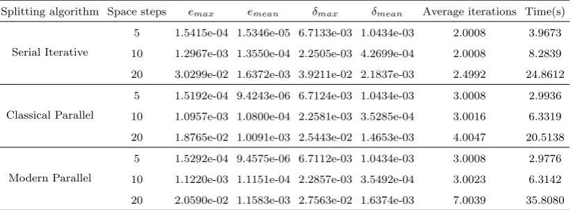
Splitting algorithm Space steps emax emean δmax δmean Average iterations Time(s)
Serial Iterative
5 1.5415e-04 1.5346e-05 6.7133e-03 1.0434e-03 2.0008 3.9673 10 1.2967e-03 1.3550e-04 2.2505e-03 4.2699e-04 2.0008 8.2839 20 3.0299e-02 1.6372e-03 3.9211e-02 2.1837e-03 2.4992 24.8612
Classical Parallel
5 1.5192e-04 9.4243e-06 6.7124e-03 1.0434e-03 3.0008 2.9936 10 1.0957e-03 1.0800e-04 2.2581e-03 3.5285e-04 3.0016 6.3319 20 1.8765e-02 1.0091e-03 2.5443e-02 1.4653e-03 4.0047 20.5138
Modern Parallel
5 1.5292e-04 9.4575e-06 6.7112e-03 1.0434e-03 3.0008 2.9776 10 1.1220e-03 1.1151e-04 2.2857e-03 3.5492e-04 3.0023 6.3142 20 2.0590e-02 1.1583e-03 2.7563e-02 1.6374e-03 7.0039 35.8080 Table 11
Results of the directional decomposition using the second order scheme for the spatial discretization, with 1280 time subin-tervals and different number of spatial steps
The parallel splittings obtain better results in error and temporal cost than the serial method in almost all cases. The utilization of fourth order approximations for the spatial derivatives gives less error, mainly for small number of spatial intervals.
The temporal cost increases between linearly and quadratically with the number of spatial steps, being higher for the fourth order scheme.
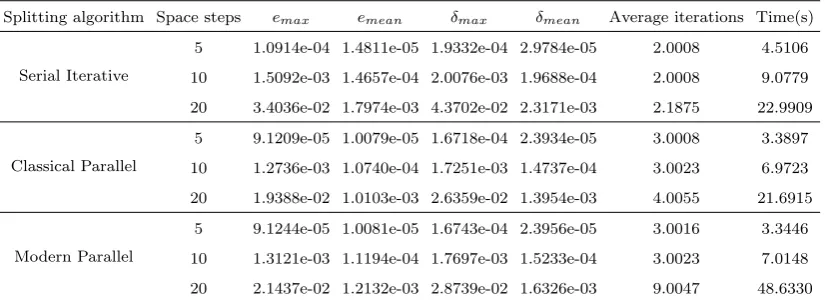
Splitting algorithm Space steps emax emean δmax δmean Average iterations Time(s)
Serial Iterative
5 1.0914e-04 1.4811e-05 1.9332e-04 2.9784e-05 2.0008 4.5106 10 1.5092e-03 1.4657e-04 2.0076e-03 1.9688e-04 2.0008 9.0779 20 3.4036e-02 1.7974e-03 4.3702e-02 2.3171e-03 2.1875 22.9909
Classical Parallel
5 9.1209e-05 1.0079e-05 1.6718e-04 2.3934e-05 3.0008 3.3897 10 1.2736e-03 1.0740e-04 1.7251e-03 1.4737e-04 3.0023 6.9723 20 1.9388e-02 1.0103e-03 2.6359e-02 1.3954e-03 4.0055 21.6915
Modern Parallel
5 9.1244e-05 1.0081e-05 1.6743e-04 2.3956e-05 3.0016 3.3446 10 1.3121e-03 1.1194e-04 1.7697e-03 1.5233e-04 3.0023 7.0148 20 2.1437e-02 1.2132e-03 2.8739e-02 1.6326e-03 9.0047 48.6330 Table 12
Results of the directional decomposition using the fourth order scheme for the spatial discretization, with 1280 time subin-tervals and different number of spatial steps
– Convection and diffusion decomposition:
Here, we decompose to an explicit part, which is the convection, and into an implicit part, which is the diffusion.
A(u)u=−1/2u(∂xu+∂yu)−1/2(∂xu+∂yu), (77)
Bu=1
2µ(∂xxu+∂yyu) +f(x, y, t). (78)
Tables 13 and 14 analyze the convergence of the different splitting methods for the convection and diffusion decomposition varying the time step.
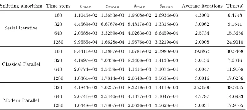
Splitting algorithm Time steps emax emean δmax δmean Average iterations Time(s)
Serial Iterative
160 1.1984e-02 1.3870e-03 2.2076e-02 3.0691e-03 3.7250 5.2347 320 4.8721e-03 6.7652e-04 1.0137e-02 1.6865e-03 3.0062 8.3601 640 2.1637e-03 3.3484e-04 5.2782e-03 1.0112e-03 2.0031 10.6301 1280 1.0151e-03 1.6667e-04 3.1179e-03 6.7675e-04 2.0008 21.1887
Classical Parallel
160 9.7517e-03 1.4278e-03 1.9648e-02 3.1946e-03 10.1000 7.0953 320 4.5454e-03 7.1452e-04 9.9089e-03 1.7712e-03 5.0125 7.0217 640 2.1597e-03 3.5723e-04 5.3681e-03 1.0580e-03 4.0031 10.9344 1280 1.0506e-03 1.7865e-04 3.2100e-03 7.0114e-04 3.0016 16.4434
Modern Parallel
320 4.5794e-03 7.1442e-04 9.9479e-03 1.7711e-03 9.6687 13.3257 640 2.1612e-03 3.5716e-04 5.3734e-03 1.0579e-03 4.8344 15.4879 1280 1.0537e-03 1.7866e-04 3.2137e-03 7.0116e-04 3.0047 17.1489 Table 13
Results for the convection diffusion decomposition using the second order scheme for the spatial discretization with 10 spatial subintervals and different number of temporal steps
of the convection and diffusion decomposition, in each part of the split, they appear derivatives in both directions, preventing the solution in blocks. In the fourth order case, the modern parallel algorithm with 160 temporal steps diverges.
Splitting algorithm Time steps emax emean δmax δmean Average iterations Time(s)
Serial Iterative
160 1.1045e-02 1.3653e-03 1.9508e-02 2.6934e-03 4.3000 6.4748 320 4.4569e-03 6.6767e-04 8.4817e-03 1.3315e-03 3.0062 9.1641 640 2.0588e-03 3.3259e-04 4.0263e-03 6.6459e-04 2.5734 15.3656 1280 9.9555e-04 1.6628e-04 1.9676e-03 3.3219e-04 2.0008 24.9010
Classical Parallel
160 8.4411e-03 1.3887e-03 1.6781e-02 2.7980e-03 39.8875 30.5468 320 4.1997e-03 7.0339e-04 8.3408e-03 1.4133e-03 5.0156 7.6316 640 2.0774e-03 3.5459e-04 4.1414e-03 7.1074e-04 4.0047 11.9168 1280 1.0361e-03 1.7814e-04 2.0640e-03 3.5636e-04 3.0016 17.6236
Modern Parallel
320 4.1843e-03 7.0237e-04 8.3219e-03 1.4119e-03 25.3500 39.5635 640 2.0741e-03 3.5440e-04 4.1377e-03 7.1047e-04 4.7797 14.6983 1280 1.0348e-03 1.7807e-04 2.0636e-03 3.5628e-04 3.0031 17.9165 Table 14
Results for the convection diffusion decomposition using the fourth order scheme for the spatial discretization with 10 spatial subintervals and different number of temporal steps
The dependence on the spatial step is analyzed in tables 15 and 16. The behavior is similar to the case of the directional decomposition, presenting an increment of the estimated error with the number of spatial subintervals for a fixed time step. In the second order scheme, the δ-errors decrease with the space step. In the fourth order scheme, theδ-errors are lower, but they slightly increase when the space step decreases. For this scheme, the modern parallel algorithm with 20 spatial steps diverges. The temporal cost is relatively high in the case of 20 subintervals, due tho the computational overhead for dealing with big matrices.
Splitting algorithm Spatial intervals emax emean δmax δmean Average iterations Time(s)
Serial Iterative
5 5.6621e-04 1.0099e-04 8.0418e-03 1.2428e-03 2.0008 12.6049 10 1.0151e-03 1.6667e-04 3.1179e-03 6.7675e-04 2.0008 25.1408 20 1.5741e-03 2.1460e-04 3.1037e-03 5.2448e-04 2.0016 244.2272
Classical Parallel
5 6.4980e-04 1.1055e-04 8.2248e-03 1.2617e-03 3.0008 9.1133 10 1.0506e-03 1.7865e-04 3.2100e-03 7.0114e-04 3.0016 19.2526 20 1.4562e-03 2.2646e-04 2.9778e-03 5.4990e-04 4.0039 244.5342
Modern Parallel
5 6.4782e-04 1.1048e-04 8.2242e-03 1.2617e-03 3.0016 9.0470 10 1.0537e-03 1.7866e-04 3.2137e-03 7.0116e-04 3.0047 19.5866 20 1.4709e-03 2.2651e-04 2.9890e-03 5.4993e-04 6.0141 339.3991 Table 15
Results for the convection diffusion decomposition using the second order scheme for the spatial discretization with 10 temporal steps and different number of spatial subintervals
The use of order approximations to the space derivatives has little influence in the results of the algorithm.
– Balanced decomposition: We decompose into:
A(u)u= (1−) (−1/2u∂xu−1/2∂xu+µ∂xxu) +(−1/2u∂yu−1/2∂yu+µ∂yyu) +f(x, y, t), (79)
B(u)u=(−1/2u∂xu−1/2∂xu+µ∂xxu) + (1−) (−1/2u∂yu−1/2∂yu+µ∂yyu) + (1−)f(x, y, t).(80)
Splitting algorithm Time steps emax emean δmax δmean Average iterations Time(s)
Serial Iterative
5 6.0051e-04 1.0212e-04 1.1690e-03 2.0887e-04 2.0008 14.2460 10 9.9555e-04 1.6628e-04 1.9676e-03 3.3219e-04 2.0008 25.2884 20 1.4979e-03 2.1332e-04 2.8794e-03 4.2570e-04 2.3289 290.9178
Classical Parallel
5 6.7972e-04 1.1140e-04 1.3249e-03 2.2717e-04 3.0008 10.6702 10 1.0361e-03 1.7814e-04 2.0640e-03 3.5636e-04 3.0016 18.2544 20 1.3859e-03 2.2483e-04 2.7619e-03 4.5066e-04 4.0047 268.6941
Modern Parallel
5 6.7894e-04 1.1130e-04 1.3246e-03 2.2718e-04 3.0016 10.2447 10 1.0348e-03 1.7807e-04 2.0636e-03 3.5628e-04 3.0031 18.4238 Table 16
Results for the convection diffusion decomposition using the fourth order scheme for the spatial discretization with 1280 temporal subintervals and different number of spatial steps
has the same behavior for values of which are symmetric with respect to 0.5. The results are quite uniform forin the range [−0.1,1.1] whereas for other parameter values, the method diverges. Only the classical parallel algorithm obtains the result for = 2, whereas the serial iterative method even fails for= 1.1 in the second order as well as in the fourth order schemes.
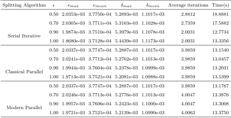
Splitting Algorithm emax emean δmax δmean Average iterations Time(s)
Serial Iterative
0.50 2.0353e-03 3.7750e-04 5.2893e-03 1.1017e-03 2.8812 18.8881 0.70 2.0305e-03 3.7711e-04 5.3163e-03 1.1028e-03 2.7359 17.5882 0.90 1.9874e-03 3.7510e-04 5.3979e-03 1.1078e-03 2.0031 12.7734 1.00 1.8680e-03 3.7128e-04 5.4439e-03 1.1173e-03 2.0031 13.3356
Classical Parallel
0.50 2.0337e-03 3.7747e-04 5.2887e-03 1.1017e-03 3.9859 13.1540 0.70 2.0241e-03 3.7712e-04 5.2762e-03 1.1013e-03 3.9859 13.0457 0.90 1.9944e-03 3.7604e-04 5.2378e-03 1.0999e-03 3.9859 13.2031 1.00 1.9713e-03 3.7521e-04 5.2081e-03 1.0988e-03 3.9859 13.5399
Modern Parallel
0.50 2.0337e-03 3.7747e-04 5.2887e-03 1.1017e-03 3.9859 13.1767 0.70 2.0246e-03 3.7713e-04 5.2776e-03 1.1013e-03 4.0047 13.3876 0.90 1.9957e-03 3.7606e-04 5.2423e-03 1.1000e-03 4.0047 13.3008 1.00 1.9721e-03 3.7521e-04 5.2139e-03 1.0990e-03 4.0062 13.3750 Table 17
Results for the balanced decomposition using the second order scheme for the spatial discretization with 640 temporal subintervals and different values of parameter
We fix the parameter = 0.9 for the analysis of the method. Table 19 compare the results of the considered splitting algorithms for different number of temporal steps using the fourth order schemes, respectively. The fourth order scheme provides better approximations than the second order one. The parallel methods behave better than the serial method for more than 160 temporal steps.
Finally, we compare the temporal cost of the different combinations of algorithms for different num-ber of time steps and 10 space subintervals. The results are shown in table 20. But for the case of 160 time steps, the classical parallel algorithm obtains the best results for the different analyzed decompo-sition methods. For 1280 time steps, the modern parallel algorithm also outperforms the serial iterative algorithm.
Here, we have the benefit, e.g., for small= 0.1, we have nearly a directional decomposition scheme. Based on the6= 0, we stabilize the scheme.
Remark 5.4 We also compared the computational time of the serial iterative, classical parallel iterative and modern parallel iterative method. We obtain a speedup for the parallel versions of a factor nearly
Lclass ≤L, if we apply L-processors. For the modern parallel version, we obtain with the same accuracy
Splitting Algorithm emax emean δmax δmean Average iterations Time(s)
Serial Iterative
0.50 2.0372e-03 3.7851e-04 4.1693e-03 7.5936e-04 2.8953 18.0265 0.70 2.0322e-03 3.7806e-04 4.1578e-03 7.5847e-04 2.7594 17.4235 0.90 1.9852e-03 3.7580e-04 4.0627e-03 7.5404e-04 2.0031 14.1016 1.00 1.8577e-03 3.7189e-04 3.8137e-03 7.4641e-04 2.0031 12.6249
Classical Parallel
0.50 2.0351e-03 3.7850e-04 4.1684e-03 7.5935e-04 4.0000 13.0915 0.70 2.0238e-03 3.7818e-04 4.1532e-03 7.5894e-04 4.0000 12.7921 0.90 1.9891e-03 3.7724e-04 4.1063e-03 7.5767e-04 4.0000 14.7150 1.00 1.9620e-03 3.7651e-04 4.0699e-03 7.5671e-04 4.0000 12.7658
Modern Parallel
0.50 2.0351e-03 3.7850e-04 4.1684e-03 7.5935e-04 4.0000 12.9446 0.70 2.0237e-03 3.7817e-04 4.1532e-03 7.5892e-04 4.0047 13.3572 0.90 1.9872e-03 3.7717e-04 4.1051e-03 7.5759e-04 4.0062 12.9882 1.00 1.9573e-03 3.7639e-04 4.0660e-03 7.5656e-04 4.0062 12.7415 Table 18
Results for the balanced decomposition using the fourth order scheme for the spatial discretization with 640 temporal subintervals and different values of parameter
Splitting Algorithm Time steps emax emean δmax δmean Average iterations Time(s)
Serial Iterative
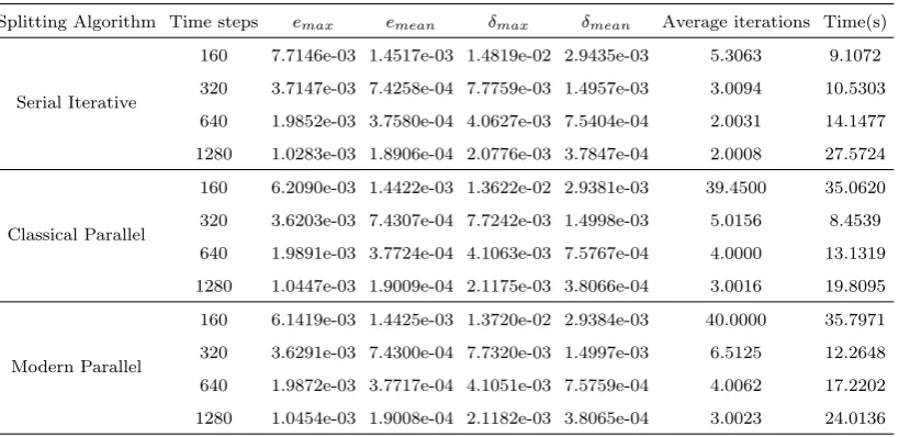
160 7.7146e-03 1.4517e-03 1.4819e-02 2.9435e-03 5.3063 9.1072 320 3.7147e-03 7.4258e-04 7.7759e-03 1.4957e-03 3.0094 10.5303 640 1.9852e-03 3.7580e-04 4.0627e-03 7.5404e-04 2.0031 14.1477 1280 1.0283e-03 1.8906e-04 2.0776e-03 3.7847e-04 2.0008 27.5724
Classical Parallel
160 6.2090e-03 1.4422e-03 1.3622e-02 2.9381e-03 39.4500 35.0620 320 3.6203e-03 7.4307e-04 7.7242e-03 1.4998e-03 5.0156 8.4539 640 1.9891e-03 3.7724e-04 4.1063e-03 7.5767e-04 4.0000 13.1319 1280 1.0447e-03 1.9009e-04 2.1175e-03 3.8066e-04 3.0016 19.8095
Modern Parallel
160 6.1419e-03 1.4425e-03 1.3720e-02 2.9384e-03 40.0000 35.7971 320 3.6291e-03 7.4300e-04 7.7320e-03 1.4997e-03 6.5125 12.2648 640 1.9872e-03 3.7717e-04 4.1051e-03 7.5759e-04 4.0062 17.2202 1280 1.0454e-03 1.9008e-04 2.1182e-03 3.8065e-04 3.0023 24.0136 Table 19
Results for the balanced decomposition with= 0.9 using the fourth order scheme for the spatial discretization with 10 spatial subintervals and different number of temporal steps
Remark 5.5 Based on balancing the decomposition of the operators with, we also obtain the benefit of the classical and modern parallel iterative splitting method with larger time-steps and more iterative steps to improve the accuracy. We can accelerate the speed of computations with the parallel versions and obtain speed ups with the modern parallel version.
6. Conclusion
Derivative approximation
Time steps 2nd order 4th order 2nd order 4th order 2nd order 4th order Splitting method Directional decomposition Convection Diffusion dec. Balanced decomposition
Serial Iterative
160 2.7961 3.1916 5.2347 6.4748 10.7499 9.1072
320 3.2505 3.5150 8.3601 9.1641 10.2080 10.5303 640 5.5462 5.4186 10.6301 15.3656 14.0321 14.1477 1280 8.4610 9.1334 21.1887 24.9010 29.1536 27.5724
Classical Parallel
160 3.2553 10.8616 7.0953 30.5468 9.4198 35.0620
320 2.7616 2.9691 7.0217 7.6316 9.1697 8.4539
640 4.4090 4.6626 10.9344 11.9168 14.8338 13.1319 1280 6.4774 6.9907 16.4434 17.6236 21.0049 19.8095
Modern Parallel
320 4.3984 5.9235 13.3257 39.5635 9.5343 12.2648 640 4.4004 5.8144 15.4879 14.6983 13.1658 17.2202 1280 6.4701 6.9861 17.1489 17.9165 21.9695 24.0136 Table 20
Cost in time of the different algorithms.
benefit of the parallel resources.
In future, we consider more real-life problems and extend the parallel iterative methods to stochastic differential equations.
Acknowledgment:
Preparation of this paper was partly supported by the project of Generalitat Valenciana Prome-teo/2016/089 and PGC2018-095896-B-C22 of the Spanish Ministry of Science and Innovation.
References
[1] I. Farago and J. Geiser. Iterative Operator-Splitting methods for Linear Problems. International Journal of Computational Science and Engineering, 3(4), 255-263, 2007.
[2] A. Frommer and D.B. Szyld. On asynchronous iterations. J. Comput. Appl. Math., 123:201–216, 2000.
[3] J. Geiser. Iterative Splitting Methods for Differential Equations. Numerical Analysis and Scientific Computing Series, Taylor & Francis Group, Boca Raton, London, New York, 2011.
[4] J. Geiser. Multi-stage waveform Relaxation and Multisplitting Methods for Differential Algebraic Systems. arxiv:1601.00495 (http://arxiv.org/abs/1601.00495), January 2016.
[5] J. Geiser.Multicomponent and Multiscale Systems: Theory, Methods, and Applications in Engineering. Springer, Cham, Heidelberg, New York, Dordrecht, London, 2016.
[6] J. Geiser. Picards iterative method for nonlinear multicomponent transport equations. Cogent Mathematics, 3(1), 1158510, 2016.
[7] J. Geiser. Iterative Splitting Methods for Coulomb Collisions in Plasma Simulations. arxiv:1706.06744 (http://arxiv.org/abs/1706.06744), June 2017.
[8] T. Ladics and I. Farago. Generalizations and error analysis of the iterative operator splitting method. Cent. Eur. J. Math., 11(8):1416-1428, 2013.
[9] R. Jeltsch and B. Pohl.Waveform Relaxation with Overlapping Splittings. SIAM J.Sci.Comput., 16(1):40-49, 1995. [10] D.P. O’Leary and R.E. White. Multi-splittings of matrices and parallel solution of linear systems. SIAM J. Algebraic
Discrete Methods, 6:630–640, 1985.
[11] U. Miekkala and O. Nevanlinna. Convergence of dynamic iteration methods for initial value problems. SIAM J. Sci. Stat. Comput., 8: 459-482, 1987.
[12] U. Miekkala and O. Nevanlinna.Iterative solution of systems of linear differential equations. Acta Numerica, 5: 259-307, 1996.
[13] S. Vandewalle. Parallel Multigrid Waveform Relaxation for Parabolic Problems. Teubner Skripten zur Numerik, B.G. Teubner Stuttgart, 1993.
[14] D. Yuan and K. Burrage. Convergence of the parallel chaotic waveform relaxation method for sti systems. Journal of Computational and Applied Mathematics, 151: 201-213, 2003.