A Comparative Study of Classification Algorithms to Analyse Biological Data sets

Available online:

http://edupediapublications.org/journals/index.php/IJR/

A Comparative Study of Classification Algorithms to Analyse

Biological Data sets

Kommareddy Roja Rani & Dr G Lavanya Devi

1

_{M.Tech CST-Bioinformatics, CS&SE Department, Andhra University, Visakhapatnam}

[email protected]

2

_{Assistant Professor, CS&SE Department, Andhra University, Visakhapatnam}

[email protected]

Abstract:

Data mining is an area of computer science with a huge prospective and it is the process of discovering or extracting information from large database or data sets. Classification also can be implemented through different number of approaches or algorithms. The main theme is applying classification algorithms on the considered breast cancer data set. The theme explains about Decision tree, Bayesian classification, Support vector machines and K-Nearest neighbor algorithms and comparison between these four algorithms can be done with the help of R Programming language, which is a open source software. For the comparison of the results, we have used accuracy, error rate, sensitivity, and specificity to find out from the confusion matrix or error matrix.

Keywords

Classification; Decision tree; Naïve bayes; K-nearest neighbor; Support vector machines; Breast cancer

1.

Introduction

Breast cancer is the second leading cause of death among women and it is the second stage of lung cancer [1]. The health and medical sector is more in need of data mining today. By using various data mining methods, valuable information can be extracted from large data base and that can help the medical practitioner to take decision, and improve health services. There are few arguments that can support the use of data mining in health sector for breast cancer like early detection, early avoidance, and indication based medication, rectifying hospital data errors [2]. For statistical analysis, graphical representation and reporting, a programming language named R is used, which provides a software environment. It is freely available under the GNU General Public License, and pre-compiled binary versions are provided for various operating systems like Mac, Linux and Windows. The main reason behind using R programming is helps researchers like us to implement and compare data

mining techniques very easily on real or synthetic data. R is free software distributed under a GNU-style copy left, and an official part of the GNU project called GNU’s.

Breast cancer is a malignant or benign tumor, inside breast, wherein cells divide and grow without control [4]. Scientists have tried to know the exact reason behind breast cancer, as there are few risk factors which increase the like childhood of a woman developing breast cancer. Age, Genetic and Hereditary problems are some factors being considered for breast cancer [3].

Treatments of breast cancer are divided into two types, local and systematic. Surgery and radiation are comes under local type of treatments whereas chemotherapy and hormone therapies are examples of systematic therapies. For getting best results, both treatments are used together in different variations as per the patient and disease intensity [9].

2.

Classification Algorithms

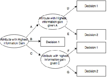
A. Decision Tree

Available online:

http://edupediapublications.org/journals/index.php/IJR/

because it is strong enough for data distribution. Here, in this used ID3 classifier for the dataset. It is a collection of pruned decision tree. ID3 has been well established for relatively small datasets. Efficiency becomes an issue of concern when these algorithms are applied to the mining of very large real-world databases. The pioneering decision tree algorithms that we have discussed so far have the restriction that the training tuples should reside in memory [6].

Fig 1: Decision Tree

B. Bayes classification

Bayesian classifier is a statistical classifier as well as a supervised learning method. It will predict class membership probabilities. It provides useful perception for understanding and assessing many learning algorithms. It calculates explicit probabilities for hypothesis and it is robust to noise in input data. When Bayesian classifier is applied to large database, it shows high accuracy and speed. The values of other attributes as the attribute value on a given class are independence to each other, the effect of this can be assumed by the naive Bayesian classifiers. This assumption is called class-conditional independence. For this purpose, the Naive Bayesian classification is used for testing [6]. The determination of the posterior probability is best defined using Bayes’ theorem.

P (H|X) = P (X|H) P (H)/ P (X)

C. Support Vector Machines

The data set teaches support vector machine to classify the new data as for classification or regression problems, supervised machine learning algorithm also known as support vector machine (SVM) is been used. It works by classifying the data into different classes by finding a line (hyper plane) which separates the training data set into classes. To maximize the distance between the various classes

that are involved in linear hyper planes, the support vector algorithm is been used and this is referred as margin maximization.

SVM’s are classified into two categories: Linear SVM’s – In linear SVM’s the

training data i.e. classifiers are separated by a hyper plane.

Non-Linear SVM’s – In non linear SVM’s it is not possible to separate the training data using a hyper plane. For example, the training data for face detection consists of group of images that are faces and another group of images that are not faces (in other words all other images in the world except faces). The training data is too complex to find a representation for every feature vector which is not possible under this condition. Dividing the set of faces sequential from the set of non-face is a complex task.

D. K-Nearest Neighbor

K-Nearest Neighbor (K-NN) classifier is also known as a distance based classifier. Nearest neighbor classifiers are based on analogy learning. So that means, it is comparing given test tuples with training tuples that are similar to it. The unknown tuple is assigned to most common class among its K-nearest neighbors. When K = 1, the unknown tuple is assigned the class of the training tuple that is closest in the pattern space. It is also used for numeric prediction, that is, it returns real-value prediction for unknown tuple [5]. This method is also called the lazy learner method.

Fig 2: K-Nearest Neighbor

3. Implementation

A. Data mining in breast cancer comparison

Four different classification algorithms i.e. Decision tree (ID3), Naïve Bayes, K-Nearest Neighbor, and Support Vector Machine have been used to analyze data.

B. Data source

Available online:

http://edupediapublications.org/journals/index.php/IJR/

we have used dataset of UCI Machine Learning Repository [8]. This dataset has 569 instances. It contains 31 attributes and 1 class attribute. As we did class distribution, there are 357(62.7%) benign class distribution and 212(37.25%) malignant class distribution. No missing values are there in the dataset. To gives description of attributes of breast cancer dataset [11].

C. Performance study of Algorithms on dataset

 Number of instances: 569

 Number of attributes: 32 (ID, diagnosis, 30 real-valued input features)

 Attribute information 1) ID number

2) Diagnosis (B = benign, M = malignant)

Ten real-valued features are computed for each cell nucleus:

a)Radius b) Texture

c) Perimeter d) Area e) Smoothness f) Compactness g) Concavity h) Concave points i) Symmetry j) Fractal dimension

Several of the papers listed above contain detailed descriptions of how these features are computed [12]. All feature values are recoded with four significant digits.

 Missing attribute values: none

 Class distribution: 357 benign, 212 malignant

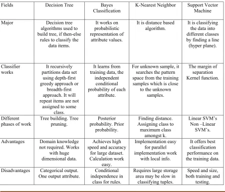
4. Comparison between the Different Classifiers

As shown in Table 1, based on different criteria, the comparison between the four algorithms Table 1 Comparison of Classifiers

Fields Decision Tree Bayes

Classification K-Nearest Neighbor Support Vector Machine

Major Decision tree

algorithms used to build tree, if then-else

rules to classify the data items.

It works on probabilistic representation of

attribute values.

It is distance based

algorithm. It is classifying the data into different classes by finding a line (hyper plane).

Classifier

works partitions data set It recursively using depth-first greedy approach or

breadth-first approach. It will repeat items are not

assigned to some class.

It learns from training data, the

independent conditional probability of each

attribute.

For unknown sample, it searches the pattern space from the training samples which is close

to the unknown samples.

The margin of separation Kernel function.

Different

phases of work Tree building. Tree pruning. probability. Prior Posterior probability.

Finding distance. Assigning class to

maximum class amongst k.

Linear SVM’s Non –Linear

SVM’s. Advantages Domain knowledge

not required. Works with huge dimensional data.

Achieves high speed and accuracy

for large dataset. Calculation work

easy.

Implementation easy for parallel implementation work

with local info.

It offers best classification performance on the training data. Disadvantages Categorical output.

One output attribute. independence in Conditional class for rules.

Requires large storage area may be slow in

classifying tuples.

Speed and size, both training and

Available online:

http://edupediapublications.org/journals/index.php/IJR/

Confusion matrix or error matrix:

A confusion matrix is obtained to calculate accuracy, error rate, Sensitivity and Specificity. Confusion matrix is a matrix representation for the classification [6]. It is shown in Table 2

 True Positives (TP): these are in which we predicated yes, and they do have the disease.

 True Negatives (TN): we predicted no, and they don’t have the disease.

 False Positives (FP): We predicted yes, but they don’t actually have the disease.  False Negatives (FN): We predicted no, but

they actually do have the disease.

The formula shown below is used to calculate accuracy, error rate, sensitivity, and specificity.

TABLE 2. Confusion Matrix

Classified as Classified as not Healthy Healthy

Actual Healthy TP FN

Actual Not FP TN

Healthy

Accuracy = (TP + TN) / (TP+FP+TN+FN) Error rate = (FP+FN)/ (TP+FP+TN+FN) Sensitivity=TP / (TP-FN)

Specificity=TN/ (TN-FP)

5. Results

Table 3. Performance Study of Algorithms of Total Data

Classifie r(569 instance

s)

Algorit hms implem

ented

Accu racy

Err or rate

Sensit ivity

Specif icity

Bayes Classific

ation

Naïve Bayes

94.02 %

5.9 7%

94.24 %

93.62 % Support Radial 98.24 1.7 99.90 95.20

Vector

Machine (rbfdot) Basis % 0% % %

K-Nearest Neighbo

r

--- 96.66

% 3.33% 99.43% 91.98%

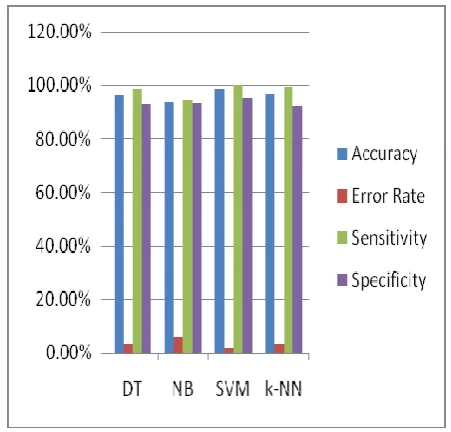
Table 3 represents the accuracy, error rate, sensitivity, and specificity for different classification techniques that have been implemented on total data set. Figure 3 represents the Support Vector Machines is superior algorithm compare to other three.

Fig 3: Comparison of Accuracy, Error rate, Specificity, Sensitivity of Total Data.

Table 4. Performance Study of Algorithms of Training Data

Classifi er(569 instanc es)

Algorit hms implem

ented

Accu racy

Error rate

Sensi tivity

Spec ificit y

Decisio n Tree

ID3 97.20 %

2.76 %

97.16 %

97.3 5% Bayes

Classifi cation

Naïve

Bayes 94.47% 5.50% 95.01% 93.43% Suppor

t Vector Machin

e

Radial Basis (rbfdot)

99.24 %

0.70 %

98.84 %

Available online:

http://edupediapublications.org/journals/index.php/IJR/

K-Nearest Neighb

or

--- 96.98

% 3.01% 98.22% 95.37%

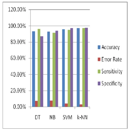
Table 4 represents the accuracy, error rate, sensitivity, and specificity for different classification techniques that have been implemented on training data set (70%). Figure 4 represents the Support Vector Machines is superior algorithm compare to other three.

Fig 4: Comparison of Accuracy, Error rate, Sensitivity, Specificity of Training Data. Table 5. Performance Study of Algorithms of Test

Data

Classifi er(569 instance

s)

Algorit hms implem

ented

Accu racy Error

rate

Sensit

ivity Specificity

Decisio

n Tree ID3 92.98% 0% 7.0 96.33% 87.09% Bayes

Classifi cation

Naïve

Bayes 92.39% 0% 7.6 91.42% 93.93% Support

Vector Machin

e

Radial Basis (rbfdot)

95.90

% 9% 4.0 95.14% 97.07%

K-Nearest Neighb

or

--- 97.07

% 0% 2.9 96.90% 97.40%

Table 5 represents the accuracy, error rate, sensitivity, and specificity for different classification techniques that have been implemented on test data set (30%). Figure 5 represents the Support Vector Machines is superior algorithm compare to other three.

Fig 5: Comparison of Accuracy, Error rate, Sensitivity, Specificity of Test Data.

CONCLUSION

Several data mining classification techniques can be applied for the identification and prevention of breast cancer among patients. In this, we used four different data miming classification methods for prediction of breast cancer. Comparison is done using different parameters for the prediction of cancer. But for superior prediction, we focus on accuracy, error rate, sensitivity, and specificity. Our studies filtered all the algorithms based on accuracy and error rate. We came up with conclusion that support vector machine is a superior algorithm.

REFERENCES

[1] U.S. Cancer Statistics Working Group.

United States Cancer Statistics: 1999–2008 Incidence and Mortality Web-based Report. Atlanta (GA): Department of Health and Human Services, Centers for Disease Control.

[2] V.Karthikeyani, I Parvin, K.Tajudin,

Available online:

http://edupediapublications.org/journals/index.php/IJR/

disease prediction. International journal of computer application 2012.12.26-31

[3] Jerez-Aragone ´s JM, Gomez-Ruiz JA,

Ramos-Jimenez G, Munoz-Perez J, Alba-Conejo E. A combined neural network and decision trees model for prognosis of breast cancer relapse. Artif Intell Med.

[4] Jiawei Han and Micheline Kamber, “Data

Mining Concepts and Techniques” , third edition, Morgan Kaufmann Publishers an imprint of Elsevier

[5] Deepa Rao, Phoebe Zhao, Breast cancer

Porject proposal

[6] Tin Kam Ho, "The random subspace

method for constructing decision forests," Pattern Analysis and Machine Intelligence, IEEE Transactions on , vol.20, no.8,

pp.832,844, Aug 1998 doi:

10.1109/34.709601

[7] Delen, D. (2009), Analysis of cancer data: a data mining approach. Expert Systems,

26: 100–112. doi:

10.1111/j.1468-0394.2008.00480.x.

[8] Using Cancer data set from UCI repository

data set ,the URL

address:\\WWW.UCI.com\\

[9] Presentations of Baysian classification can

be found in Duda, Hart, and Stork [DHS01], Weiss and Kulikowski [WK91], and Mitchell.

[10]For an analysis of the predictive power of na¨ıve Bayesian classifiers when the class-conditional independence assumption is violated, see Domingos and Pazzani [DP96]

[11]W.H. Wolberg, W.N. Street, and O.L.

Mangasarian. Machine learning techniques to diagnose breast cancer from fine-needle aspirates. Cancer Letters 77 (1994) 163-171.

[12] Computerized breast cancer diagnosis and