www.ijiset.com
Joint Channel Estimation Based on Compressive Sensing for
Multi-User Massive MIMO-OFDM Systems
Menglu SunP
*
P
Yingzhi ZhaoP
*
*Chongqing Key Lab of Mobile Communications Technology, Chongqing University of Posts and Telecommunications, Chongqing 400065, P. R. China
Abstract
With the number of transmit antennas increases largely in Massive MIMO systems, the training and feedback overhead for the acquisition of channel state information (CSI) at the transmitter becomes rather overwhelming. In order to solve the problem of huge overhead of channel estimation, this paper utilizes a new CSI estimation scheme and the hidden joint sparsity structure in multi-user channel impulse response vectors and thus proposes a joint channel estimation algorithm based on compressive sensing (CS) technique for orthogonal frequency division multiplexing systems. In this scenario, after the base station transmits training signals to each user, the users directly send back the observed signals to the base station and then the joint CSI acquisition problem could be realized at the base station. Then, by using the distributed sparse property of Massive MIMO-OFDM systems, the recovery of the CSI of all users can be realized by the joint channel estimation algorithm. Simulation results show that the proposed algorithm can achieve accurate CSI with lower overhead and complexity.
Keywords: Massive MIMO-OFDM, channel state information, joint channel estimation,
1. Introduction
Massive MIMO (multiple-input multiple-output) refers to the idea of equipping base stations with hundreds of antennas and has become one of the key techniques of 5G
wireless communicationP
[1]
P
. It can boost the system capacity and energy efficiency by orders of magnitude through effectively utilizing of the space resources. To fully realize the technological superiority of massive MIMO as well as for signal detecting and precoding, the accurate CSI is essential both in uplink and downlink channels. For the system of time division duplexing (TDD), the CSI can be obtained from uplink channel by using the channel reciprocityP
[2]
P
. While TDD has the advantage on channel estimation, the frequency division duplexing (FDD) can provide more efficient communications with symmetric
traffic and low latency than TDDP
[3]
P
, which is more popular in current cellular networks. Hence, it is important to
provide efficient solution of CSI estimation for FDD massive MIMO systems.
In conventional channel estimation for FDD MIMO systems, the BS firstly sent pilot signals to users in the downlink and each user then conduct their own channel estimation by using least square (LS) or minimum mean square error (MMSE). And then the estimated channel is fed back to the BS via dedicated uplink channels. Since the number of pilots grows with the same scale of transmit antennas at the BS, the pilot overhead for channel estimation is prohibitively high which will be a big challenge for massive MIMO-OFDM systems. In recent years, as many studies have shown that the channel impulse response (CIR) in wireless communication systems is sparse, that is, most of the energy of CIR is focused on fewer paths. Thus, it is natural to combining the compressive reconstruction algorithm with the sparse channel estimation, which can achieve better estimation performance than traditional channel estimation methods by using the same number of pilot symbols.
At present, different compressive sensing based approaches have been proposed in recent years. Many researchesP
[4,5]
P
applied greedy pursuit algorithms for sparse channel estimation as it can recovery the original channel frequency domain response with high probability, but it may also cause the large pilot overhead with the increase of the number of antennas in massive MIMO-OFDM systems. Besides, some other researches utilized the hidden sparsity in CIR vectors and thus improve the estimation performance than traditional greedy pursuit algorithms. For instance, in [6], a new model of massive MIMO-OFDM system is considered by utilizing the temporal correlation in different OFDM symbols and proposes the local common sparsity channel estimation algorithm (LCS) to achieve the higher estimation efficiency and accuracy than traditional LMMSE algorithm and greedy pursuit algorithms.
www.ijiset.com
channel estimation method by using the joint sparsity for multi-user MIMO-OFDM systems.
The rest of this paper is structured as follows: In the
second part is the establishment of multi-user
MIMO-OFDM systems; the second part is the design of joint sparsity channel estimation algorithm; the fourth part is the scheme of the simulation analysis. Finally, we conclude the paper in part 5.
Notations: Uppercase and lowercase boldface denote
matrices and vectors respectively. The operators ,
, , , , are the transpose, conjugate
transpose, inverse, pseudo inverse, cardinality, indicator function, big-O notation operator respectively. And
denotes the rank of matrix ; denotes the
Frobenius norm.
2. System Model
2.1 MIMO-OFDM system model
As is shown in Figure 1, we consider a MIMO-OFDM
system with transmit antennas and receive antennas,
and assume the channel between the th transmit antenna
and the th receive antenna is a frequency selective
fading channel.
Figure1. MIMO-OFDM system model
Assume that each OFDM symbol contains
subcarriers, where the number of pilot subcarriers is
and the number of data subcarriers is . The
position of the pilot subcarriers in the first OFDM symbol
is expressed as , which is randomly
selected from the sequence of . During the
data transmission procession, the OFDM modulation
signal is sent by the transmit
antenna, and then after the inverse discrete Fourier transform (IDFT), the pilots are multiplexed with data in the frequency domain. In addition, a cyclic prefix (CP) is finally added to each signal to avoid inter-symbol interference (ISI). At the receive antenna, each user firstly removes the CP and then performs the DFT transformation to get the received pilot signals.
Assuming that the channel parameters are constant during an OFDM symbol, then the signal received by the each user is expressed as:
(1)
where , and is the
discrete channel frequency response of the th
transmitting antenna and the th receiving antenna;
is the Gaussian white noise .
In the Rayleigh fading channel, the traditional channel estimation method requires that the pilots of the different antennas of the MIMO-OFDM system should be orthogonal to each other, 41Tfor simplicity,41T we assume that
only one antenna transmit pilots in the time-frequency
recourse elementsP
[7]
P
. Then the pilot symbols received by
the th receiving antenna can be expressed as:
(2)
where is the received
pilot signal in single antenna, is the
transmitted pilot signal; is the time-domain CIR vector
with size of and is assumed to be sparse,
is a DFT matrix and its element is
, is a partial DFT
matrix which is selected from the rows from the DFT
matrix with its index corresponding to the ,
is the coordinate matrix corresponding to
the columns selected from the unit matrix,
is the Gaussian white noise,
is the observation matrix and is defined as
. In addition, to ensure that the
www.ijiset.com
subcarriers is randomly selected
from the sequence , and the pilot signal is a
Gaussian random matrix.
2.2. Joint sparsity of Multi-user MIMO-OFDM
System
Suppose there are K users in massive MIMO-OFDM
system, as the number of scatters is limited near the base station, the transmitted signals from the base station to different users often passes through the common scatters, especially for the users with similar distance. So the CIR vectors of different users have the similar channel delay and thus their CIR vectors exhibit the common sparsity. Besides, 41Tdue to the rich scatters near each user41T, when the
signal arrives at different users through different scatters, each channel of user has a different arrival delay, thus their CIR vectors exhibit the individual sparsity. Figure 2 shows the joint structure of multi-user system, where the scatter 1 and the scatter 3 in the Figure 2(a) are the individual scatter for user 1 and user K, respectively, and the scatter 2 is the common scatter for all users. Therefore, the CIR vectors in Figure 2(b) has both the common sparse location and individual sparse location.
Figure2. Joint sparse model of Multi-user systems
Due to the time correlation of MIMO-OFDM systems, that is, the locations of domain locations usually vary slowly in time which can be considered as constant during certain time duration. Thus, in several continuous OFDM symbol time, the time common sparsity of time-domain CIR vector can be expressed as:
(3)
where is the CIR vector for each user
in R continuous OFDM symbols.
Besides, during each OFDM symbol, the common sparsity of CIR vectors among different users can be expressed as:
(4)
As shown in Figure 3, except for the common sparsity in different CIR vectors for all users, the remaining sparse locations of them are different. The total sparse
support of different users is expressed as and the
size of common support set and the individual support set
satisfy and ,
respectively.
Figure3. Joint sparsity structure of CIR vectors
Based on the system model of equation(2) and the above sparse properties, the joint multi-user massive MIMO-OFDM system model in can be formulated as:
(5)
where is the channel impulse response vector
of the k-th user in the n-th OFDM symbol.
In order to take advantage of the joint sparse features of multi-user massive MIMO-OFDM systems and to reduce the pilot overhead, we adopt an improved estimation scheme that each user directly feeds back the pilot observation after they receives the pilot signal, then we can get the stacked receive pilot vectors for each user as:
(6)
Since the CIR vectors within different OFDM symbols have the same sparsity (see Eq. (3)), the combined CIR vectors can be reorganized into a block sparse matrix:
(7)
As is a sparse block matrix, and its
www.ijiset.com ( ) ( ) 1 1 ( ) 1 N ( ) ( )
[ ... ] , 1
CIR CIR k k k k k N R k K = + ≤ ≤ d z
r Ψ Ψ
d z
(8)
where RNP R, ( 1, 2, , )
i i NCIR
×
∈ =
Ψ C is the observation
matrix corresponding to reordered vector[ 1( ), , ( ) ]
CIR
k k T
N
d d .
Considering the Rayleigh fading channel model with
the maximum Doppler frequency as fd, then the temporal
correlation of complex gain is given as:
(
)
( ) ( ) ( )
[ ] 1 ,
k k k H i R R
i j CIR
R R
P for i j
E i j N
for i j × × = = ≤ ≤ ≠ 0 J
d d (9)
where
P
i( )k=
E
[| (
h
nk) |]
i 2is the variance of the i-th elementof CIR vector, JR R× is the covariance matrix with its
( , )m n element asJ0(2
π
f T m nd s( − )).Thus, the channel estimation problem of the joint sparsity multi-user MIMO-OFDM system is the problem
of using the observation matrix
{
Ψi,1≤ ≤i NCIR}
and thepilot observations of multiple users to obtain the combined
time-domain CIR vector
{
r
( )k,1
≤ ≤
k
K
}
, which can beexpressed as the following joint model:
(1) (2) ( )
1 1 1
(1) (2) ( )
2 2 2
(1) ( ) 1
(1) (2) ( )
(1) ( )
1 1
(1) ( )
[ ,..., ] [ ... ]
(10)
CIR
CIR CIR CIR
K
K K
N
K
N N N
K K R R = +
d d d
d d d
r r Ψ Ψ
d d d
z z
z z
3. Joint Channel Estimation Algorithm
In order to solve the channel estimation problem of equation(10), we firstly use the temporal estimation
algorithm to calculate the common support setΩCof all
CIR vectors, and then calculate the remaining individual support set of each user which we called the joint channel estimation algorithm (JCE).
3.1. Temporal channel estimation algorithm
The algorithm firstly uses the greedy pursuit method to calculate the correlation between the observation matrix
i
Ψ and the residual matrix to find out the index of the
largest correlation, with the common support set updated at each iteration, the common support set is utilized to calculate the LMMSE correlation coefficient which will
finally obtain the estimated CIR vectors{dˆn i,,∀i}after S
times of iteration.
The specific steps are shown as follows:
1: Input: rn,
{
Ψi,∀i}
,{
Pi ,∀i}
,S, j,2: Output:
{
dn i,,∀i,}
3: Initialize M:=rn,Ω:=∅,j=1
4: Repeat the following steps until the iteration index =j S:
5: Find the index of largest correlation:
max: arg max H i F i
i = Ψ M
6: Update the common support set: Ω Ω:= {imax}
7: Compute the LMMSE estimation:
1
, : [ ,( ) ] [ ( ) ],
H H
n i E n i n E n n i
−
= ∀
W d r r r
[ ,( ) ] : ,
0,
H H i R R i n i n
P for i
E otherwise × ∈ =
J Ψ Ω
d r
[ ( ) ] : 2
P P
H H
n n i i R R i w RN RN i
E P ×
σ
×∈
=
∑
+Ω
r r Ψ J Ψ I
8: Calculate the estimated CIR vector:
, ,
ˆ : , 1
n i =Wn i n ≤ ≤i NCIR
d r
9: Update the residual and the iteration index, and then return to the step 5:
,
ˆ
: n i[ n i]
i∈ = −
∑
M r Ψ d
Ω
, j= +j 1
3.2. Joint channel estimation algorithm
The algorithm flow is shown as follows:
, k,C,i
MInitializationΩ Ω
Find the top indexes of maximum correlation value
Determine The common support set and update
the residuals
Iteration index
C k
i≥S −S Yes
No
Stop iteraton and output the estimated CIR
Calculate the correlation between each user residual
and the measurement matrix to get the
Calculates the estimated CIR through the temporal estimation algorithm and Update the residualM( )k C Ω k Ω k S
Initialize the individual sparse support set{ e: }
k= C
Ω Ω
www.ijiset.com
In the algorithm flow, the specific step for calculate
common sparsityΩCof all users are explained as follows:
Firstly, we initialize the residual ( ): ( )k
k =r
M , individual
sparse support set
{
Ωk:= ∅ ∀, k}
, common sparse supportset ΩC:= ∅, and the number of iterations s=1.
Secondly, compute the iteration calculation for SC
times:
1. Using the greedy pursuit method to calculate the
correlation between each user's residual M( )k and the
observation matrix {Ψi,∀i} , and then find the top
|
|
k C
S
−
Ω
′
index of maximum correlation value:: arg max H ( ) 2, | | | e|
k′ = Λ k F Λ = −Sk C
Ω Ψ M Ω (11)
2. Find out the index j with the largest number of
occurrences for different users and then update the estimated common support set:
{ }
1
arg max
k K e e
C = C j
∑
k= I j∈Ω′Ω Ω (12)
where ( )
k
IΩ′ x is the indicator function and is defined as:
1 , ( )
0 ,
k
k
k
if x
I x
if x
′
′ ∈
= ∉ ′
Ω
Ω
Ω (13)
3. Update the residual of all users, and estimate the channel frequency domain with the indexes corresponding to common sparse support set by using the temporal channel estimation algorithm:
(1) ( ) (1) ( )
: [ , , ] [ , , ]
e C
K K
i i i i∈
= −
∑
M r r Ψ d d
Ω
(14)
Thirdly, after SCtimes of the iteration, we can obtain
the common sparse support set, then carry out the update
of each user's sparse support setΩC, and then use the
temporal channel estimation to obtain the final channel
estimation{ˆ( )k, , }
i ∀i k
d .
5. Simulation analysis
In this part, we use the Matlab simulation platform to fully verify the performance of the proposed algorithm. In
order to prove that our proposed JCE41T algorithm is feasible
and effective,41T we compare it with typical greedy pursuit
algorithm and the LCS algorithm proposed in [6]41T, and set
the Oracle algorithm as the low bound. Besides, we also verify the effect of common sparsity and individual sparsity on estimation performance. Through the
simulation, it can show that 41Tthe proposed JCE algorithm
has better channel estimation performance than traditional estimation algorithms, which is of great usefulness for multi-user massive MIMO-OFDM systems.
The main parameters are shown in Table 1.
Table 1Simulation parameters Simulation parameters value
number of users 20 number of subcarriers 20 spacing of subcarriers 15kHz
Doppler frequency 70Hz maximum delay spread 4.88μs time interval of OFDM symbols 0.5ms length of CIR vector 150
channel sparsity SRCR=7, S=15 signal to noise ratio(SNR) 20dB
iteration times 500
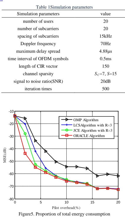
Figure5. Proportion of total energy consumption
Figure5 compares the mean square error (MSE) of
several algorithms to verify the 41Tfeasibility and
effectiveness41T of JCE algorithm. It can be seen from the
figure that the JCE algorithm is slightly better than the LCS algorithm and is far superior to the OMP algorithm. This is because the LCS algorithm and the OMP algorithm perform the recovery of separate support set for each user without using the common sparsity of all users which leads to the poor ability to recover the original signal with less observation.
In order to verify the efficiency and time complexity of different algorithms, we compute the operating time of various algorithms. For the typical OMP algorithm, to solve the problem of channel estimation in the model (10), it utilizes iteration estimation based on the direct selection of the support set which has the time complexity of
3 ( P)
O R KSN . The LCS algorithm proposed in [6] estimate
the individual support set of each user and has the time
complexity of 3 3 3
( P CIR P)
O R KSN +R N SN . The proposed JCE
algorithm firstly estimate the common sparsity and then estimate the remaining individual support set and has the
0 5 10 15 20
-80 -70 -60 -50 -40 -30 -20 -10
Pilot overhead(%)
MS
E
(d
B
)
www.ijiset.com
time complexity of 3 3 3
( P P )
O R KSN +R SN . The comparison of
time complexity of different algorithms is shown in Table 2:
Table 2 Comparison of time complexity of different algorithms Algorithms Time complexity
OMP 3
( P) O R KSN
LCS 3 3 3
( P CIR P)
O R KSN +R N SN
JCE 3 3 3
( P P )
O R KSN +R SN
Figure6. node mobility ratevs packet delivery ratio
Figure 6 verifies the operating time of various algorithms. It can be seen from the figure that the JCE algorithm has slightly less computational complexity than the LCS algorithm as the JCE algorithm compute the LMMSE estimation based on the obtaining of common sparsity. The LCS algorithm separately recoveries the support set for each user which requires higher number of calculations. For the OMP algorithm, even though it has a lower computing time due to the simple structure, it has a big gap to the oracle algorithm as shown in Figure5 which confirms that the overall performance is still poor. Combining the Figure 5 and Figure 6, it can get the conclusion that the proposed JCE algorithm has the big advantages for the channel estimation in joint sparse model.
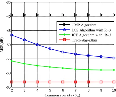
Figure 7 verifies the effect of common sparsity on the channel estimation performance of different algorithms with the pilot overhead set to 4%. It can be seen from the figure that when the user's individual sparseness remains a
constant and the common sparsity SRCR keeps increasing,
the estimation performance of JCE algorithm and LCS change better, whereas the estimation performance of
OMP algorithm does not change with the increasing of SRCR.
This is because the JCE algorithm takes advantage of the common sparsity of different users, and the probability of correct recovery becomes higher with the increasing of the number of common support set. However, the OMP
algorithm is related to the overall sparsity S and has
nothing to do with the common sparsity and therefore does not change with the increasing of SRCR..
Figure7. node mobility ratevs packet network lifetime
Figure8. node mobility ratevs network throughput
Figure 8 verifies the effect of individual sparsity on the channel estimation performance of different algorithms with the pilot overhead set to 4%. As can be seen from the figure, with the individual sparsity increasing, the estimation performance of the various algorithms becomes worse. The reason can be derived from the theory of compressive sensing, which illustrates that if the sparsity increases, the required observations should be increased in order to ensure the channel estimation performance. Therefore, the estimated performance of the system will
become worse with the increase of S under the same
dimension of pilot observation.
0 5 10 15 20
0 0.5 1 1.5 2 2.5 3 3.5 4 4.5
Pilot overhead(%)
T
ime
(s
)
LCS Algorithm JCE Algorithm OMP Algorithm
2 3 4 5 6 7 8 9 10
-65 -60 -55 -50 -45 -40 -35
Common sparsity (SC)
MS
E
(d
B
)
OMP Algorithm LCS Algorithm wirh R=3 JCE Algorithm with R=3 OracleAlgorithm
14 15 16 17 18 19 20 -80
-75 -70 -65 -60 -55
Individual sparsity(S)
MS
E
(d
B
)
www.ijiset.com
5. Conclusions
To solve the problem of overwhelming estimation overhead in massive MIMO-OFDM systems, this paper utilizes the hidden sparsity in channel impulse response vectors for multi user systems and proposes a joint sparsity channel estimation algorithm. Experimental results show that the proposed algorithm reduces the estimation overhead as well as time complexity and obtain the better estimation performance with comparison to the typical greedy pursuit algorithm.
Acknowledgments
This work was supported in part by the Program for Cheung Kong Scholars and Innovative Research Team of China (IRT1299) and funded by Chongqing key laboratory (CSTC2013yykfA40010).
References
[1] L. Lu, G. Y. Li, A. L. Swindlehurst, A. Ashikhmin, and R. Zhang “An overview of massive MIMO: Benefits and challenges,” IEEE Journal of Selected Topics in Signal Process., vol. 8, no. 5, pp. 742-758, Oct. 2014. [2] T. L. Marzetta, “Noncooperative cellular wireless with unlimited numbers of BS antennas,” IEEE Trans. Wireless Commun., vol. 9, no. 11, pp. 3590–3600, Nov. 2010.
[3] F. Rusek, D. Persson, B.K. Lau, and F. Tufvesson, “Scaling up MIMO: Opportunities and challenges with very large arrays,” IEEE Signal Process. Mag., vol. 30, no. 1, pp. 40-60, Jan. 2013.
[4] Karabulut G Z, Youngacoglu A. Sparse channel estimation using orthogonal matching pursuit algorithm [C]// IEEE 60th Vehicular Technology Conference. Los Angeles: IEEE Press, 2004: 3880-3884. [5] Donoho D L, Tsaig Y, Drori I, et al. Sparse solution of underdetermined linear equations by stagewise orthogonal matching pursuit[J]. IEEE Transactions on Information Theory, 2012, 58(2): 1094-1121.
[6] Jun W C, Byonghyo S, Seok H C. Downlink Pilot Reduction for Massive MIMO Systems via Compressed Sensing[J]. IEEE communication Letters, 2015, 19(11): 1889-1892.