Representing multifunctional cities: density and diversity in space and time

Representing

Multifunctional

Cities: Density and

Diversity in Space

Michael Batty

Elena Besussi

Kees Maat

Jan Jaap Harts

http://www.casa.ucl.ac.uk/working_papers/paper71.pdf

WORKING P

A

PER SERIES

ISSN: 1467-1298 © Copyright CASA, UCL

71

Representing Multifunctional Cities: Density and Diversity in

Space and Time

Michael Batty

1

, Elena Besussi

1

, Kees Maat

2

, and Jan Jaap Harts

3

[email protected] , [email protected], [email protected], [email protected] 1_{Centre for Advanced Spatial Analysis, University College London,}

1-19 Torrington Place, London WC1E 6BT, UK

2_{OTB Research Institute for Housing, Urban and Mobility Studies}

Delft University of Technology, P.O. Box 5030, 2600 GA Delft, The Netherlands

3_{Urban Research Centre, Utrecht University}

P.O. Box 80.115, 3508 TC Utrecht, The Netherlands

10 November 2003

Abstract

In this paper, we define measures of urban diversity, density and segregation using new data and software systems based on GIS. These allow us to visualise the meaning of the multifunctional city. We begin with a discussion of how cities have become more segregated in their land uses and activities during the last 200 years and how the current focus is on reversing this trend through limiting urban sprawl and bringing new life back to the inner and central city. We define various indices which show how diversity and density manifest themselves spatially. We argue that multifunctionalism is a relative concept, dependent upon the spatial and temporal scale that we use to think about the mixing and concentration of urban land uses. We present three examples using spatially smoothed indicators of diversity: for a world city – London, for a highly controlled polycentric urban region – Randstad Holland, and for a much more diffusely populated semi-urban region – Venice-Padua-Teviso. We conclude by illustrating that urban diversity varies as people engage in different activities associated with different land uses throughout the day, as well as through the vertical, third dimension of the city. This impresses the point that we need to understand multifunctional cities in all their dimensions of space and time.

Acknowledgements

Diversity and Density:

Concentration and Segregation of Urban Functions

By all accounts, the European medieval city was a place teaming with different activities where people accomplished their daily tasks in close proximity to one another. Through economic necessity, most activities clustered close together, literally on top of one another and what segregation existed was highly ritualised through the institutionalised power of church and state. All this was changed by the industrial revolution. Although new populations were concentrated in factory towns, this congestion was much more uniform than hitherto. As wealth began to increase, people and activities sought more space and the heterogeneity of the city in history began to reduce.

In the 20th _{century, this process has accelerated in the quest to deconcentrate activities in}

the search for more living and working space. This has been made economically possible by keeping urban activities linked together through new transport technologies with lower costs. Urban sprawl has lead to less diversity and greater segregation of populations according to income while economic activities have no longer needed to be as concentrated as close to one another as they have been in the past. This has led to highly specialised nodes such as edge cities appearing as a counterpart to the familiar decline of the city centre or downtown, particularly in North America (Besussi and Chin, 2003). Planning policies that sought to reduce such diversity were widely applied during the 20th century, ranging from the segregation of pedestrians from vehicles at the urban design scale, to the movement of industries away from their traditional cores through policies such as new towns and growth poles at the regional.

During the last half century, there are few who have questioned this almost unwitting association of planning policy with the economic momentum towards a decentralised, dispersed urban world. Although Jane Jacobs (1961) has been a lone voice in arguing that cities should fight to be more like their medieval counterparts than the kinds of soulless, low density forms that have become the norm, the idea that cities might be once again higher density, with mostly mixed rather than segregated uses, appears to be gaining ground. The diseconomies of urban sprawl are well known but transport congestion, the need to reduce pollution, and the need for more liveable environments are all being used to argue that the multifunctional city is now a distinct reality. Given the fact that modern economies are largely based on soft activities, on the knowledge economy, and on services rather than manufacturing or manual labour, the economic conditions appear more favourable for high density, mixed use location than at any time during the last 200 years.

examples we will use to demonstrate how such diversity can be measured, are based on two-dimensional map representations. However once we have presented these, we will illustrate how the 24 hour city changes our view of diversity and how the third dimension important in very large cities, mainly in their centres, must be central to extending our understanding of this concept. The indicators that we introduce are all designed to provide us first and foremost with a deeper understanding of the extent to which our cities are already multifunctional. But in developing these new ways of visualising urban structure provides us with the opportunity for using the same kinds of measure to visualise urban futures which are radically different in functional terms.

Measuring Multifunctionality through Spatial Indicators

In talking of multifunctional cities, we make the assumption that more than one activity or function exists in the same location and/or at the same time, which only strictly holds if we consider a neighbourhood or time interval in which these activities exist together. We will examine this in more detail later but for now, it is clear from our previous discussion, that multiple functions are often associated with higher densities as well as a greater range or mix of individual activities existing side by side. As densities get lower, activity is more spread out and less distinct activities exist in the same place; at high densities, many different activities can exist simultaneously simply due to their crowding. Density is usually defined as the normalised areal count of an activity; in contrast, mix can be best measured as a simple count of different activities in any one place or time.

Let us define the total number of activities or land uses as K and the amount of an activity k in a place i as a(i,k). The variable b(i,k) shows the existence of that variable

k at i; that is if a(i,k)>0, then b(i,j)=1, otherwise b(i,j)=0. The simplest measure of diversity δ(i) is a direct or raw count of the number of activities at i, that is

∑

= _kb i k i) (, ) (

δ which varies from 0 where there is no activity of any kind to K where all the activities in the entire system exist in that place. These and all subsequent statistics might be normalised to sum to 1 or expressed as differences from their means but none of these manipulations change their intrinsic meaning.

The diversity measure δ(i) does not take direct account of density but to create such a measure, some kind of normalisation must take place to enable different amounts of the activity to be compared. One way to do this is to express the amount of activity as a proportion of its maximum, and then sum these variables across all activities which exist in each place. We call this the density-diversity d(i)=

∑

_k

(

a(i,k) max_ia(i,k)

)

which also varies over the same range from 0 to K. When d(i)= K, this means that in the place i, the volume and mix of activities is the greatest it can be with the maximum volume of each activity existing there.

to )d(i as d~(i)=

∑

_k~a(i,k). Using this instead of the maximum ratio gives a statistic with the same interpretation as the raw count δ(i) but in density terms. A statistic which takes this place-based density-diversity from its regional mean has been used in the Amsterdam study below as a measure of separation or segregation and this is given as d(i)~

∑

_k a~(i,k)−

(

∑

_ka(i,k)

∑

_ika(i,k)

)

. When this statistic is equal to 0, then the mix of activities is identical to the regional mix. This difference increases the more the place is unlike the regional mix. Many other measures of diversity might be used ranging from location quotients, shift-share measures, and entropy statistics. One of the key issues however is not so much the actual statistics used but the shapes of the distribution that occur for it is this that provides our understanding of how multifunctionality varies in space and time.

Scale and Aggregation in the Definition of Multifunctionality

Whether or not a place has more than one function – land use or activity – depends on the size of that place. If places are too small, measured at the level of centimetres, say, then no human activity can take place that is recognisable in terms of urban geography. The finest scale that we usually deal with is at the scale of the person where only a single activity can take place at any one time. As we get larger scales and spaces, more and more activities that differ can take place. When we aggregate everything to one space – the level of the region, say – all the functions that can take place do take place there. The finest-scale places we will consider here are at the level of postcode geography which in the UK and Holland represent, on average, cells or polygons of about 50 metres square. Below this we might deal with land parcels on which more than one activity can take place but at coarsest scales such as blocks, block groups, and census tracts, then a much wider variety of activities is possible.

As we aggregate some places in suburban areas, these remain homogenous while other areas, particularly city centres, become more heterogeneous. What spatial analysis teaches us is that multifunctionality is a relative concept depending upon the way we define space, and its spatial variation will depend intrinsically on the scale used. We must always have in mind that wherever we examine the variation in activity a(i,k), there is another level of activity distribution at a finer spatial scale where there is no multifunctionality whatsoever. If this scale is j, then what we are doing is working with data which has been defined around a neighbourhood of i, Z(i), where we are aggregating the basic data from this scale to form a(i,k)=

∑

_j∈Z(i)a(j,k).

average a(i,k)=

∑

_j∈Z(i)a(j,k) 9. A more controlled method for achieving such smoothing is by using a kernel density estimator (KDE) such as the one in the proprietary GIS software ArcView (Mitchell, 1999). This is based on Silverman’s (1986) quadratic and it is used to generate different levels of surface smoothing choosing different sizes of bandwidth – akin to different window sizes.

With a specific kernel function, it is the value of the bandwidth, also called the

smoothing parameter, that determines the degree of averaging in the estimate of the density function. The possibility of “manipulating” the results of the KDE through the application of different bandwidths and functions can be empirically translated into testing different assumptions about the spatial behaviour of a particular variable such as its distance decay effects. In Figure 1, we show some simple smoothing of density data for employment in Amsterdam while in Figure 2 we show the effect of smoothing some population data for part of the Venice region using increasing bandwidths, These examples show how important it is to be clear about the effect of spatial aggregation on the interpretation of density and diversity. In the example we develop below, these kinds of function are used extensively to display and interpret spatial variations of multifunctionality. These surface modelling techniques also offer the possibility of estimating the values of a density or indicator at each location in space for which information is not available. By making assumptions on the spatial distribution of that particular variable or indicator around points of known value, such smoothing can be accomplished (Bracken and Martin 1989; Martin, Langford et al. 2000).

Map-Based Visualisations of Multifunctionality

Figure 1: Housing Density in Amsterdam at 250 by 250 metres (left) Aggregated and Smoothed to a 750m x 750m Grid Cell (right) (scale E-W 15kms)

a) area-based density b) bandwidth = 100m

d) bandwidth = 500m f) bandwidth = 1000m

In our second example, we examine two additional perspectives on diversity: first through density differences or mismatches between aggregate employment and population; second through variations in the intensities of land use which are used to construct an index of diversity based on weighted absolute values of employment and population. The urban region is based on the cities of Venice, Padua and Teviso which is often referred to in the Italian literature as the “diffuse city” (Indovina, Savino et al. 1990), a homogenous distribution of low density developments, punctuated by a few relatively small urban centres. This data set, unlike that of London, is based on assigning urban activity types – individual values of population and employment for the three major economic sectors (industrial, commercial-office, and service) available for built-up objects based on land parcels and building blocks – to the centroids of small census tracts. This is then used as the seed data for surface modelling, our standard technique of representation in this paper.

The mismatch between aggregate employment and population densities implies a strong separation of work from home as reflected particularly in commuter mobility patterns (Gottlieb and Lentnek 2001). In Figure 4, we compare two surfaces in the periphery of the Venice region based on density values for population a(i,1) and employment

) 2 , (i

a , standardised with respect to their mean values. The spatial autocorrelation between these surfaces is immediately clear and this seems to imply that the lower the density of population, the less the number of jobs in the same place, thus reinforcing the notion that sprawl implies homogeneity and lack of diversity. To make this more explicit, we have taken three transects along the main transport routes within this region. We show these in Figure 5 and these bear out our initial impressions. These again are useful visualisations taken from GIS which indicate the power of this technology for understanding different perspectives on density and diversity. These profile graphs can be interpreted as individual “signatures” of the functional organisation of activities along those routes. In the first one (Figure 5a), the profile is highly fragmented but without any significant interruption in the average density: lower levels of population densities are counterbalanced by higher levels of employment. Despite the continuity of the built-up areas, this transport corridor presents several “patches” where residential uses prevail over employment activities and vice versa. The second and third cases (Figures 5b and 5c) presents average densities. However the profiles show that along these two routes, areas of high density are separated by areas of lower-than-average densities, more typical of a strictly polycentric structure than of urban sprawl.

Figure 3: Spatial Variation in Diversity [δ(i)]in a World City: London

(a) Greater London showing the main town centres with diversity on a blue (low) to deep red (high scale) : E-W 40kms

(b) Central London showing the City and the West End: note the low diversity of Regents Park and Hyde Park: E-W 8.5kms

(a) Population Density Surface (b) Employment Density Surface

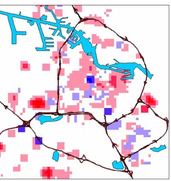
Our last example is for Amsterdam. This is a core city within Holland’s Randstad which has been subject to intensive planning controls for many decades. Here we will show how the indices of density and diversity based on [d(i)] and on segregation [d(i)] can be used to show not only the spatial variation of mixed uses in the core cities, the peripheral urban region, and the ‘green heart’ but also the trends in mixed use over a six year time period. In Figure 7, we show measures of density-diversity and segregation for Amsterdam where it is clear that, like central London, the centre is highly diverse. Single use specialised areas such as the docks and residential enclaves are clearly picked up by the index of segregation. This is part of a larger study which sheds light on spatial structure by examining variations and developments in dispersal of urban activities, mix of uses, density and diversity in urban areas throughout the Netherlands (Maat and Harts, 2001; Harts, et al., 2002). Analyses were performed at the detailed level of 250m for 1990 and 1996 entailing the application of grid cell and cluster analysis to four spatial databases from which typologies of urban environments were generated. In Figure 8, the shift in the diversity between 1990 and 1996 is shown where it is clear that areas in the centre decline in heterogeneity while other sub-centres become more diverse.

Maat and Harts (2001) have used these measures to classify urban environments in the Netherlands into 15 different categories based on the composition of their uses. The class divisions in the typology were based on cluster analysis. This technique classifies the data in such a way that the environments are internally as homogeneous as possible and, at the same time, differ as much as possible from one another. A distinction was drawn between urban and rural areas; then urban areas were further classified into urban environments. The developments were analyzed by comparing the trends of 1990 with those of 1996. To create a comparable typology for 1990, the classification criteria (based on the boundaries for each variable) of the 1996 typology were applied to the 1990 variables.

a b c Figure 5: Density Profiles based on Transects between the Main Centres in Figure 4

(the largest peaks in these figures are employment densities, the lower population)

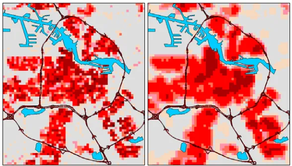
Figure 6: Density-Diversity Surfaces at Different Scales in the Venice Region (scales left to right E-W 20 kms, 8kms, and 3kms)

Figure 8: Changes in the Density-Diversity between 1990 and 1996(scale E-W 18kms) (red = increase, blue = decrease; bright = considerable change, light = limited

change)

What this analysis shows is that the whole concept of multifunctionality and mixed use is more convoluted spatially than its discussion implies. Often the argument for or against mixed use is predicated without any basis in data and although it is generally clear that suburban sprawl is much more homogeneous than previously developed residential locations closer to the urban core, this must be set against the fact that increasing wealth leads to new opportunities for developing mixed uses. Specialisation in time is also equally important; populations are now much more able to organise their working days around access to different uses and activities in time and as well as space. It is to this that we turn in concluding our brief discussion of the need for good data in generating a clear picture of how diverse our cities are becoming.

The Third and Fourth Dimensions: The Vertical City,

The 24 Hour City

Urban Area

Density

Index

Specialization

Index

Urban Environment

₁₉₉₆

[km2]

1990-96

[%] 1990-96 [%] Metropolitan centre

Urban centre

Weakly urbanized centre Concentration of services Metropolitan residential area Urban residential area

Moderately urbanized residential area Weakly urbanized residential area Business estates

Green space and sports Infrastructure

Residential area and green space Business and dwellings

Business and green space Services in countryside

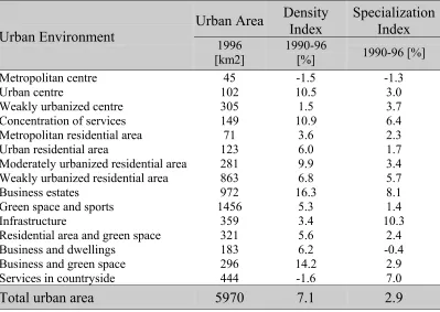
45 102 305 149 71 123 281 863 972 1456 359 321 183 296 444 -1.5 10.5 1.5 10.9 3.6 6.0 9.9 6.8 16.3 5.3 3.4 5.6 6.2 14.2 -1.6 -1.3 3.0 3.7 6.4 2.3 1.7 3.4 5.7 8.1 1.4 10.3 2.4 -0.4 2.9 7.0

Total urban area

5970

7.1

2.9

Table 1: The 15 Urban Environments in the Netherlands: Extent, Density, and Specialization 1990 – 1996

many functions associated with the volume but the association of numbers of uses with higher storeys and greater volumes is never direct. In fact in many large, declining downtowns, the highest buildings may not be in use at all and thus this kind of visualisation is crucial in understanding the economic health of high density cities.

Figure 9: The Index of Diversity (left) Mapped onto 3D Building Blocks in Central London (right)

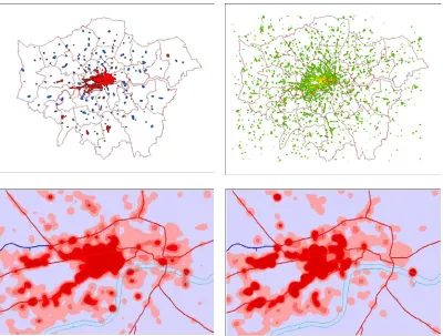
Figure 10: Classifying Diversity in 24 Hour City

(a)London’s Town centres Classified by into Night Life Hubs (red) (b) Night Life Actvitiy Based on Entertainment Employment

(c)Diversity of the Day Time Economy in Central London (d) Diversity of the Night Time Economy in Central London

Implications for Spatial Planning

All this suggests that the kinds of typology such as that for the Netherlands noted above which classify urban environments according to such measures, should be widely developed for multicultural and multinational comparisons. We may actually be quite surprised that what we consider to be homogeneous might turn out to be much more interesting and heterogeneous than physical appearance and form might imply. What we can do with the measures developed here is to test their sensitivity to changes in activities. For example, we can answer questions like: “how much less diverse would central London be if all retailing were to leave the core?” And equally well we could ask and answer questions like: “how much more diverse would central London be if certain amounts of residential population were to occupy the centre?”.

This suggests that we could examine the functional structure of more idealised forms, for example, the range of city shapes associated with the compact city idealisations developed by Italian Renaissance scholars to the musing of the modernists such as Frank Lloyd Wright and Le Corbusier and beyond to contemporary proposals as reflected in the New Urbanism. It is not very usual to speculate on what multifunctional cities might look like in terms of quantitative data concerning employment and related land use activities. But with good forecasting models that often lie behind the ideas developed here, it is possible to make small area predictions for future cities under different assumptions which imply a range of planning scenarios. In such cases, we should be able use the kinds of visualisation that we have introduced to generate useful discussion about future cities.

Although we have focused on methods for visualisation, the fact that we are able to map so many different variants of these indices also gives us the opportunity to make many contrasts between different kinds of index. We can relate these indicators to other issues of functionality and functioning, both economic and social. It would be possible to associate these to patterns of crime, deprivation, economic opportunity, local economic development potential, unemployment and so on which all correlate with multifunctionality. These are issues, however, for the future and we will conclude by returning to the immediate technical developments that our focusing on these technologies implies.

Conclusions: Next Steps

In contrast, our work on urban sprawl in the Venice region and in the Randstad, is motivated by a concern for understanding urban growth and the separation of home from work through concepts such as wasteful commuting (Martin, 2001). Sustainable planning underlies many of these ideas but in the quest to engender greater opportunities for urban living, the idea of mixed uses is increasingly attractive. However we must be clear as to the extent to which cities are changing spontaneously towards or away from such mixing. To this end, new data of the kind we have used here is essential while the need to link the fine scale geography of the city to its geometry and the move from the 2D map to the 3D model are key issues in getting to grips with the concept of the multifunctional city.

References

Batty, M. (2000) The new geography of the third dimension. Environment and Planning B, 27, pp. 483-484.

Besussi, E. and Chin, N. (2003) Identifying and measuring urban sprawl. In P. Longley and M. Batty (eds.) Advanced Spatial Analysis. Redlands, CA: ESRI Press, pp. 234-278. Bracken, I. and Martin D. (1989) The generation of spatial population-distributions from census-centroid data. Environment and Planning A, 21, pp. 537-543.

Gottlieb, P. D. and Lentnek, B. (2001) Spatial mismatch is not always a central-city problem: an analysis of commuting behaviour in Cleveland, Ohio, and its suburbs.

Urban Studies, 38(7), pp. 1161-1186

Harts, J.J., Maat, K. and H. Ottens (2002) An urbanisation monitoring system for strategic planning. In S. Geertman and J. Stillwell (eds.) Planning Support Systems in Practice. Berlin: Springer Verlag, pp. 315-329.

Indovina, F., Savino, M. et al. (1990) La Citta Diffusa. Venezia, Italia: DAEST.

Jacobs J. (1961) The Death and Life of Great American Cities. New York: Random House.

Maat, K. and Harts, J. J. (2001) Implications of urban development for travel demand in the Netherlands. Transportation Research Record, 1780, pp. 9-16.

Martin, D., Langford, M., et al. (2000) Refining population surface models: experiments with Northern Ireland Census data. Transactions in GIS, 4(4), pp. 343-357.

Martin, R. W. (2001) Spatial mismatch and costly suburban commutes: can commuting subsidies help? Urban Studies,38, pp. 1305-1318.

Silverman, B. W. (1986) Density Estimation for Statistics and Data Analysis. New York: Chapman and Hall.