A Review - LOOP Dependence Analysis for
Parallelizing Compiler
Pradip S. Devan1, R. K. Kamat2 1
Department of Computer Science, Shivaji University, Kolhapur, MH, India– 416 004 2
Department of Electronics, Shivaji University, Kolhapur MH, India – 416 004
Abstract— Business demands for better computing power
because the cost of hardware is declining day by day. Therefore, existing sequential software are either required to convert to a parallel equivalent and should be optimized, or a new software base must be written. However analyzing and detection of healthy code snippet manually is a tedious task. Loops are most important and attractive for parallelization as generally they consume more execution time as well as memory. The purpose of this paper is to review existing loop dependence analysis techniques for auto-parallelization. We present some technical background of data dependency analysis, followed by a review of loop dependence analysis. The review material focuses explicitly on dependence analysis techniques, dependence tests and their drawbacks. We conclude by discussing the nature of the review material and considering some possibility for future.
Keywords— Compiler, Parallelization, parallel computing,
loop dependence analysis.
I. INTRODUCTION
Many of the industries had followed traditional sequential programming before. Algorithms are constructed and implemented considering sequential call flow; hence only one instruction may execute at a time [1-4]. Parallel programming seems to be the most logical way to meet the current business demand. Therefore, existing traditional sequential software are either required to convert to a parallel equivalent and should be optimized, or a new software base must be written. However, both options require a skilled developer in dependence analysis. Converting these software’s in multithreaded for parallel computation increases the complexity and cost involved in software development due to rewriting legacy code, efforts to avoid race conditions, deadlocks and other problems associated with parallel programming.
Some parallel languages such as SISAL [5] and PCN [6] have found little favour with application programmers; however industries prefer to use their traditional sequential programs rather than learning a completely new language only for parallel programming. In view of this, auto-parallelization could be the best option to convert existing traditional sequential software instead of doing it manually.
Many researchers have worked on the development of automatic parallelization from different points of views. There are several well-known research groups involved in the development and improvement of parallel compilers, such as Polaries, PFA, Parafrase, SUIF etc [4,7]. Most research compilers consider FORTRAN programs only for automatic parallelization. FORTRAN programs are simpler to analyse as compared to C/C++ programs. Typical
examples are: Vienna FORTRAN, Paradigm, Polaris, SUIF compilers. Compiler should be able to reorder the sequential statements for parallelism exploitation. The challenge for such a reorder is ensuring the changed order always computes the same result for all possible inputs.
In particular, loops are a rich source of parallelism and can be used to achieve considerable improvement in efficiency on multiprocessors Therefore; we have reviewed the existing data dependence tests and algorithm for loops dependency. The review was conducted in order to locate the available literature in this field and to isolate potential research areas. The elements of data dependence computation that we consider are limited explicitly to methodologies, algorithms defined in different research papers.
II. DEPENDENCE ANALYSIS
The sequential language introduced few constrains which are not critical for preserving the computation. Finding such set of constrains is key for transforming programs to parallel one. Characterizing these constrains allow the PC to reorder execution of a program without changing its constraint. These constraints are called as dependency.A set of dependency is sufficient to ensure that program transformations do not change the meaning of actualprogram. The same results are achieved by preserving the relative order of the writes to each of the memory location in the program.
Compilers will have the ability to analyze the tasks that can be safely and efficiently executed in parallel. The code can be executed parallel in case there is no dependency in between execution path. Dependence is a relation in between the statements of program. Statement S2 is said to be dependent on S1 (S1 δ S2); if S1 must be executed before S2 to produce correct output. Dependence analysis [8,9] distinguishes between two kinds of dependence: data dependence and control dependence.
A. Data dependency:
Two statements are called data dependent whenever the variables used by one statement may have incorrect values if the statements executes in reverse order. For example; statement S2 has data dependence on statement S1 in following segment because of AREA
S1: AREA=PI*R*2 S2: VOLUME=AREA *H B. Control dependency:
example: the execution of S2 is depending on the result of statement S1.
S1: If(A!=0) { S2: B=B/A; S3: }
Both data as well as control dependency should be taken care by compiler while parallelizing any program. Data decomposition, where parallel tasks perform similar operations on different elements of the data array could be highly effective technique for parallelizing program. The dependence can be classified [12] into:
1) True dependence: S1 writes and then S2 reads from
same memory location (RAW) denoted as S1 δ S2 2) Anti-dependence: S1 reads and then S2 writes at
same memory location (WAR) denoted as S1 δ- S 2 3) Output dependence: Both S1 and S2 write at same
memory location (WAW) denoted as S1 δo S2 4) Input dependence: S1 reads memory andS2 later
reads (RAR) the same which is denoted as S1 δi S2
Consider below statements which have execution path in sequential order as a dependence classification example.
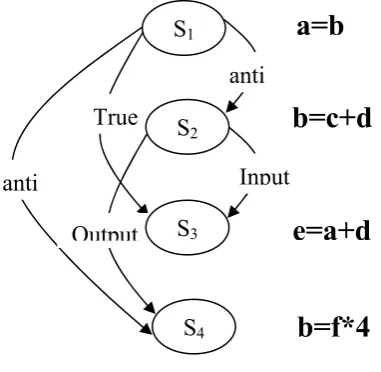
S1: a=b; S2: b=c+d; S3: e=a+d; S4: b=f*4;
The variable of each statement “variable = expression” holds the result of the statement and hence it acts as its output, while the variables in the expression are the input of the statement.
Fig 1 Shows the dependency between S1, S2, S3 and S4.
In Figure 1, the output variable of S2 (b) is being used
by statement S1 as an input variable; hence S2 is
anti-dependent on S1 (i.e. S1 δ- S2). The variable (b) is
utilized in S2 and S4 statements. Value of (b) will be f*4
after execution of S4 in sequential execution. The value
of (b) is determined by the execution order of S2and S4:
if S4 is executed before S2, the final value of (b) will
change, hence S4 is said to be output dependent on S2
(i.e. S1 δo S2). S2 and S3 are reading same variable (d);
hence S3 is said to be input dependent on S2. (i.e. S2δi
S3) Output variable (a) of S1 is being used in statement
S3 as an input; hence S3 is true dependent on S1 (i.e. S1 δ S3)
III. LOOP DEPENDENCE
Loops execute statements multiple times in a regular computation and it often contains array variable. Loops are very attractive for parallelization as generally they consume more execution time as well as memory. Detecting such loop dependencies and applying automatic transformation is a complex task. To achieve this, we need a powerful mathematical model which helps the compilers to detect dependencies and transform the input in parallel form.
The next section lists some of the terms which form mathematical base for dependency analysis.
1) Iteration vector: It represents a particular
execution of statements by setting an entry of a vector to the value of the corresponding loop induction variable.
2) Iteration space: It is a set of all possible
iteration vectors for a statement.
3) Distance vector: It indicates the distance
between iterations, denoted by σ
4) Direction vector: It indicates the corresponding
direction, basically the sign of the distance, denoted as ρ
The best way to build an understanding for these mathematical terminologies is to start with a simple example. Consider the following loop:
for (i=1;i<=3;i++) { for (j=1;j<=3;j++) { S A(i,j)=A(j,i);
} }
Iteration space [13] for above loop is {(1,1), (2,1), (2,2),(3,1), (3,2), (3,3) }. Iteration number can be calculated by using below formula:
i = (I– L+1)/S, i= iteration number
I = value of index on that
iteration
L= Lower bound
S= steps.
The lexicographic order of two iteration vectors can be succinctly summarized using distance vector and direction vectors [14].
Distance vectors [14] were first used by Kuck and Muaoka in [12, 15]. It describes dependences in between iterations. They are very crucial to determine whether loop can be executed in parallel or not. If two iteration vectors i (is the source of dependence) and iteration vector j (is the sink of the dependence) represents of dependent statements (S1 δ S2) in nested loop; then the distance vector (i,j) is
defined as vector of length such that: d(i,j)k= jk - ik
Output
S
1anti
True
anti
Input
b=c+d
a=b
e=a+d
b=f*4
S
2S
3Direction vectors were first introduced by Wolfe[16]. It is closely related to distance vector and are useful for calculating the level of loop carried dependences [17, 18]. They are mapped into direction vectors such that:
“<” if d(i,j)k> 0
D(i,j)k = “=” if d(i,j)k = 0
“>” if d(i,j)k< 0 where d(i,j)k = jk - ik
Direction vector whose leftmost non “=” component is not “<”; it means dependence doesn’t exist. It indirectly express that the sink of the dependence occurs before the source. In some cases a direction vector or distance vector alone may be insufficient to completely describe dependence and so both distance and direction vector may be required. Consider the following example:
for (i=1;i<=4;i++) { for (j=1;j<=i;j++) {
S A(I+1,J) = ...
... = A(I,J) }
}
Find the details of iteration vectors and their dependence relations for above example in TABLEI and TABLE III below:
TABLEIII
Iteration Vector (I,J) S1 S2
(1,1) A(2,1) A(1,1)
(2,1) A(3,1) A(2,1)
(2,2) A(3,2) A(2,2)
(3,1) A(4,1) A(3,1)
(3,2) A(4,2) A(3,2)
(3,3) A(4,3) A(3,3)
(4,1) A(5,2) A(4,1)
(4,2) A(5,1) A(4,2)
(4,3) A(5,2) A(4,3)
(4,4) A(5,4) A(4,4)
TABLEII
S1δ S2 Array Element
S1(1,1) δ S2(2,1) A(2,1)
S1(2,1) δ S2(3,1) A(3,1)
S1(2,2) δ S2(3,2) A(3,2)
S1(3,1) δ S2(4,1) A(4,1)
S1(3,2) δ S2(4,2) A(4,2)
S1(3,3) δ S2(4,3) A(4,3)
Arrays from TABLEIV are dependent on each other. Dependence vector for above example is (1, 0) and direction vector is (<, =).
Loop dependence can be further classified as either loop-independent or loop-carried, depending on whether it exists independently of any loop inside of which it is nested. Loop-independent flow dependence does not inhibit any parallelization of the outer loops because it will still be satisfied. Loop-carried dependences may inhibit parallelization because the simultaneous execution of different iterations may leave them unsatisfied
.
1) Loop Carried dependence:
Loop carried dependence is a dependence that arises because of the iteration of loops. Statement S2 has a
loop-carried dependence on statement S1iff S1 and S2 has
execution path and they refer to memory location M on their respective iteration i and j, where i>j. Consider below C code snippet for details:
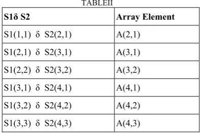
for (i=2;i<=4;i++){ S1: a(i+1)= ...
S2: ...=a(i) }
If statement S2 appears before S1 within same loop or
both S1 and S2 are same statements; then that loop-carried
dependence is called as backward. If S2 appears after S1
within loop then that loop carried dependence is called as forward.
“Level” of dependence is an important factor of loop carried dependence. Dependence level conveniently summarizes dependences and is useful for reorder transformation. Reorder transformation just changes the execution order of execution code, without any change in actual statements. It doesn’t eliminate dependences, however, it can change the ordering of the dependence e.g. change from true to anti-dependence or vice versa
Fig 2- Shows the relations between S1 and S2 for each iteration and their dependences. S1 is the source and S2 is the sink of the
dependence. S1 and S2 always execute in different iteration and they always have negative dependence vector i.e. (“<.”).
a(4
a(5) a(3)
a(4) a(2)
a(3) i=2 S1[2] S2[2]
i=3 S1[3] S2[3]
level of a loop-carried = index of the leftmost non “=” of D(i,j).
The level of dependences in,
for(i=1;i<10;i++) { for(j=1;j<10;j++) {
for(k=1;k<10;k++) {
S1 A(i,j+1,k) = A(j,j,k)
} } }
is 2 because D(i, j) is (=,<,=)for every i, j that creates a dependence.
2) Loop independent dependence:
It arises as a result of relative statement position. Thus, loop-independent dependences determine the order in which code is executed within a nest of loops. Statement S2 has a loop-independent dependence on
statement S1 if and only if S1 and S2 has execution path
within iteration and they refers memory location M on their respective iteration i and j where i=j. Dependence vector is always 0 for loop-independent dependence. Consider below C code snippet for details:
for(i=2;i<=4;i++){
S1: a(i)=...
S2: ... =a(i) }
IV. DEPENDENCE TESTING
Dependence testing is the method used to determine whether dependences exist between two subscripted references to the same array in a loop nest [19]. Loops are main source of the parallelism in any program and precise data dependence information is necessary to detect parallelism. Dependence testing is done in pairs to discover data dependences between iteration of nested loops. Dependence exists if any two iterations of the loop access same array with same subscript (i.e. the same memory location). First step of dependence testing is to partition subscripts according to their complexity, and test accordingly.
1) Partition Based Algorithm
a. Partition the subscript S into m separable and minimal coupled groups S1, S2, ...Sm for a single
reference pair enclosed in n loops with indexes I1, I2, ...
In.
b. Label each subscript as ZIV, SIV or MIV
c. For each separable subscript, apply the appropriate single subscript test (ZIV, SIV, MIV) based on the complexity of the subscript. If independence is proved, no further testing is needed else it will produce direction vectors for the indexes occurring in that subscript.
d.For each coupled group, apply a multiple subscript test to produce a set of direction vectors for the indices occurring within that group
i)If any test yields independence, no dependences exist.
ii)Otherwise merge all the direction vectors computed in the previous steps into a single set of direction vectors for two references.
iii) This algorithm is implemented in both PFC, an automatic vectorizing and parallelising compiler, as well as ParaScope, a parallel computing environment [20,21,22].
2) Merging Direction Vector:
The merge operation is simply a Cartesian product of direction/distance vectors produced by individual tests. Let us see in the below example:
for (i=0; i<N; i++) { for (j=0; j<N; j++) {
S1 A (i+1, 4) = ...
S2 ... = A (i, N);
} }
The first partition subscript (i+1, i) yields the direction vector (<) for the loop with index i. second partition subscript (4, N) doesn’t have j index and N doesn’t indirectly vary with j and hence the full set of direction vectors (*) [8] needs to be assumed. The direction vector for i and j yields the set of direction vectors {(<, <), (<, =), (<, >)}, or {(<, *)}. If one of the dependence test proves to be independence; merge is not necessary, since overall result is independence.
V. DATA DEPENDENCE TESTS
Once subscript partition is done; specific tests can be applied to determine whether dependence exists or not. Most of the dependence tests are assumed that there is data dependence exist in program if independence can’t be proved. In this way, produced parallel code can’t guarantee about safe parallelization.
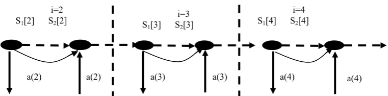
Fig 3- Shows the relation between source and sink for each iteration. S1 is the source of the dependence; S2 is the sink. S2 is always dependent on S1 in the same iteration. The number of iterations between source and sink is 0.
a(4) a(4)
a(3) a(3)
a(2) a(2)
i=2 S1[2] S2[2]
i=3 S1[3] S2[3]
These dependence tests are classified on the subscript basis.
I) Single-subscript dependence tests:
Simplest test cases are available; that can be applied on single subscripts. Some of them are discussed in below section:
1) ZIV test:
ZIV (zero index variable) subscript does not vary within any loop and hence if two expressions are not equal then the corresponding array references are independent. If independence cannot be proven, the subscript does not produce any direction vectors, and may be ignored. For example:
for (j=1; j<10; j++) {
S A[a1] = A[a2] + B[j]
}
a1, a2 are constants or loop invariant symbols. If (a1-a2)! =0,
it means Dependence doesn’t exists
2) Strong SIV Test:
Subscript for an index i is said to be strong if it has the form <ai + c1, ai' + c2>. Since the loop coefficients are
identical for each reference, a strong SIV pair maps into a pair of parallel lines. Access to common elements will always be separated by the same distance in terms of loop iterations. This dependence distancecan be calculated by the following:
d= i'-i= (c1-c2)/a
Dependence exist if d is an integer and |d|<= U-L
Let us understand below example:
for (i = 1;i<N;i++){
S1 A[i+2*N] = A[i+N] + C
}
The dependence distance d as (2N-N)/1 which simplifies to N and U-L equal to (N-1). Here N> N-1 and hence |d| > U-L. This proves there is no dependence.
3) Weak-zero and weak-crossing SIV Tests:
Subscript for an index i is said to be weak if it has the form <a1i + c1, a2i' + c2>. It always has different coefficient
where the dependence equation is a1i + c1= a2i' + c2. If one
of the coefficient is 0 (i.e. a1=0 or a2=0), the subscript is a
weak-zero SIV subscript. If a2=0; then dependence equation
reduces to i= (c2 - c1)/ a1. In this case, the dependence is
usually caused by first or last iteration that may be eliminated by loop peeling [23 - 26]. If one coefficient has exact negative value of other (i.e. a1= -a2), then the
subscript is weak-crossing SIV test and dependence equation will be i= (c2 - c1)/ 2a1. This dependence may be
eliminated by the loop splitting transformation [23 - 26].
II) Multiple Induction Variable Tests:
SIV subscripts are relatively simple linear mapping from the Z(the set of natural numbers) to Z in single loop; however MIV subscripts are much complicated as we have to do mapping from Zm to Z, where m is the number of loop induction variables appears in the subscripts. This added complexity requires sophisticated mathematics in order to accurately determine dependences. The test for MIV subscripts are
1) Delta Test
The “Delta test” [27,28] derives from the informal usage of ΔI to represent the distance between source and sink
index of I-loop. The main idea behind this test is constraints derived from SIV subscripts may be efficiently propagated into other subscripts in the same coupled group without losing any precision.
The delta test can find independence if any of its ZIV or SIV tests determine independence. If no independence is found using the ZIV and SIV tests then the delta algorithm converts all SIV subscripts into constraints, and propagated into MIV subscripts. If the propagation process results with new SIV subscripts, then the conversion is repeated until no new SIV subscripts are produced.
Next, MIV subscripts are scanned for RDIV (Restricted Double Index Variable) subscripts. RDIV subscripts have form {aj*ij + cj, ak*ik + ck}, and are similar to SIV subscripts, except that ij and ik are distinct indices. Testing the RDIV subscripts produces new constraints, which are then propagated into remaining MIV subscripts.
At the end, remaining MIV subscripts are tested subscript-by-subscript, possibly resulting in false dependences. Described procedures are performed by the Delta test algorithm [18]
2) Symbolic Test:
This test is important to deal with symbolic quantities for resolving data flow dependencies, which appear frequently in subscripts. The difference between loop-invariant symbolic additive constant (c2-c1) can be symbolically formed and simplified. The result of this simplification can then be used like a constant in order to break possible dependencies. This test can be applied on the following pair of loops which are dealing with two array references.
for (i = 1;i<N1;i++){
S1 A(a1 *i+ c1) = ……
}
for (j = 1;j<N2;j++){
S2 …… = A(a2 *j+ c2)
}
Based on above pair of loop, dependence exists if the following dependence equation is satisfied for some value of i (1 <= i<=N1) and j (1 <= j <=N2). (Assuming a1 is
greater than or equal to zero). a1 *i - a2 *j = c2 - c1
Below two possible cases can be considered in this test: a) a1 and a2 may have same signs.
As a1 and a2 are non-negative, (a1*i – a2*j) assumes its
maximum value for i= N1 and j=1 and minimum value for
i=1 and j= N1; so the dependence exist iff:
a1 - a2N2 <= c2 - c1 <= a1N1 - a2
b) a1 and a2 may have different signs.
As a2 is negative (remember we are assuming a1 is
greater or equal to 0), (a1*i – a2*j) assumes its maximum
value for i= N1 and j= N2 and minimum value for i=1 and j=
1; so the dependence existsiff:
a1 - a2<= c2 - c1 <= a1N1 - a2N2
3) The Banerjee -GCD Test:
they are identified by the function. For example – if equation (a0 + a1 *X = b0 + b1*X’) for some integer X and
X’; then (a1 *X - b1*X’) = b0 - a0. In this case (b0 - a0)
should be between upper bound (i.e a1 *max(X) - b1*
min(X’)) and lower bound (i.e. a1 *min(X) - b1* max(X’))
of given equation.
The Banerjee test requires the loops with constant bounds and also considers if statement conditions and does not analyse non-linear expressions. This test case assumes that all indices are independent; therefore if test fails to prove the same then this test does not guarantee that dependence really exists. In this extreme case GCD test can be applied.
The GCD (greatest common divisor) test [32] is based upon a theorem of elementary number theory, which states that a linear equation (a1x1 +a2x2 + ... + anxn= a0) has an
integer solution iff the gcd of the coefficients on the left-hand side of the equation (a1,a2,… an) divides the right
hand side constant(a0) [33]. For example – linear equation
(3x + 5y = 20), the gcd of the coefficients on the left-hand side of the equation (i.e. gcd(3,5)) =1 divides right hand side constant (20), it means the given linear equation may have integer solution.
Besides ignoring loop bound, the GCD test also doesn’t provide distance and direction information. Also GCD is often 1, which ends up being very conservative
.
4) The I-Test
The I-Test [34, 35], is an enhancement of Banerjee and GCD test which extends the range of applicability as well as the accuracy. The I-Test is based on the observation that most of the real solution is predicted by Banerjee test. It leads the development of set of conditions, which determines the integer value between minimum and maximum values for liner expression by using Banerjee test. These accuracy conditions [36] states the relationship between the coefficients of loop index variables and the range of values they realize, in order to guarantee that every integer value between the extreme values is achievable.The
I-Test is based on the notion of the integer interval equation:
a1 *X1 + a2 *X2 + a3 *X3 +…. an *Xn= [L, U] EQ-1
wherePk<= Xk<= Qkfor 1<=k<=n
An integer interval equation is used to denote the set of all ordinary linear equations with constantterms the integers between L and U. It has an integer solution iff at least one of the equation in the set has an integer solution, subject to the constraints. The equation and constraints in EQ-1 are equivalent to
a1*X1 + a2*X2 + a3*X3 +…. an*Xn= [a0,a0] EQ-2
where a0 is divisor by gcd(a1, a2 .. an)
The I-Test is applied starting on EQ-2. This equation is (P1,Q1;P2,Q2…. Pk,Qk)-integer solvable iff the interval
equation
a1*X1 + a2*X2 + a3*X3 +…+an-1*Xn-1 = [a0–a+n*Qk+a -n*Pk,a0– a+n*Pkk+a-nQn] EQ-3
where Pk<= Xk<=Qkfor 1<= k <= n-1
a+= a if a>0 otherwise 0 a- = a if a<0 otherwise 0
is integer solvable. The above is applied until there are no terms on the left side or the GCD test indicates that there may be a solution for interval equation. If the integer interval on the right-hand side includes zero, then a solution exists, otherwise there is no integer solution subject to the constraints.
Also if d= gcd (a1, a2 ..an); then the constraint interval
equation in EQ-1 is integer solvable iff the constrained interval equation:
a1/d1*X1 + a2/d2*X2 + a3/d3*X3 +…. an/dn*Xn= [L/d,U/d]
EQ-4 wherePk<=Xk<=Qkfor 1<=k<=n
The I-Test inherits all of the benefits of the Banerjee test, including efficiency and ability to provide direction vector information. Similarly to the Banerjee test I-Test requires constant loopbounds and can be applied only to linear subscript.
5) The Omega Test:
Omega Test [37] is an exact dependence and based on a combination of least remainder algorithm and Fourier-Motzkin variable elimination (FMVE) [26] where additional extension tests of FMVE can guarantee the existence of integer; however has worst case exponential time complexity. The input of the Omega test is a set of equalities and inequalities resulting from the subscript expressions, the iteration index bounds or the if-statement conditions; hence derivation of Knuth's [20] least remainder algorithm is used to convert these inputs into linear inequalities. GCD test and bound normalizations are applied to detect if the system is inconsistent during this initial conversion. In such cases, the test reports no dependence exists, otherwise an extension to standard FMVE is used to determine if converted linear equalities has integer solution. The variable elimination is performed on pairs of inequalities using FMVE techniques. If the resulting “real shadow” contains no integers, then the original object contains no integer, and the test reports that no solution exists. However it’s not necessarily true that the real shadow may contain integers, whereas, the original object actually contains no integers; hence Omega test calculate the subset of the real shadow called “dark shadow”. It represents the area under the original object where integer solution definitely exists. If it contains integers, then the Omega Test reports that dependence exist. But the same time if dark shadow is empty and real shadow is non-empty, Omega Test begins exhaustive search of the solution space, recursively generating and solving integer programming problem until integer solutions are either found or disproved
.
6) The Range Test:
cannot expose parallelism for these non-linear expressions [40].
The Range Test assumes that dependence exists and it always tries to disprove dependences. For a given iteration i of a loop L, the accessed array subscript range, range(i), is considered as symbolic expression; if this range doesn’t overlap with the range accessed in next iteration, i+1, then there is no dependence for L. The two ranges do not overlap if max(range(i) ) <min(range(i+1)). The Range Test disproves carried dependences between A(f(i)) and A(g(j)) for a loop L, by proving that the range of elements taken by f and g do not overlap
.
DISCUSSION AND CONCLUSION
In this review, we have concentrated on loop dependence analysis for optimization and parallelization.Data dependence analysis is the key to optimization and detection of implicit parallelism in sequential programs. Loops are most important and attractive for parallelization as generally they consume more execution time as well as memory. Dependence analysis for loop can be done by using a set of distance and direction vectors. They describe dependences between loop iterations which are necessary to discover the parallelism in a program. Hence, we have explained the data dependence techniques in details for interested readers.
The review material demonstrates the data dependence analysis techniques and most of the dependence tests which can be applied to detect loop dependence. All tests are not suitable for all loops. Still there is some scope to improve some of dependence tests. Each data dependence test has its own limitation and restriction; so different output may arise for same problems due to different reasons. The ultimate goal of this work is to understand and improve available mathematical models of data dependency analysis. Designer should consider all cases related to data dependence accuracy, efficiency of generated code during transformation of existing source code. We have discussed such issue and their respective solutions as below:
1) Loop Variant Variable
The values of loop variant variables are generally changed inside the loop nest which depends on the values of the enclosing loop indices. Compiler techniques such as induction variable substitution [43], can recognize variables which can be expressed as functions of the indices of enclosing loops and replace them with induction variables with the expressions involving loop indices. The transformation should make the relationship between variables and loop indices explicit; however such transformation may not always bepossible; but at the same time dependence test may be able to resolve problems with loop variant accurately. Consider below example:
for (I = 1; I<= N; I++) {
for (J = 1; J<= M[I]; J++) {
S1: A[I, K + J] = ...
S2: . . . = A[I, K + J + 1];
} K=2*K; }
Here value of array M[I] and K will change inside the loop nest. The value of changes in each iteration of I; however it remains same for each iteration of J. So the level of variance for these two variant variables is the level of loop I and hence loop variant expression can be determining the innermost loop. All occurrences of that expression for direction vector is of the form (=, >) for all level of variance. This technique can help to check whether loop variant variable is equal in dependence problem and can be simplified algebraic operations and can be incorporated in dependence test.
2) Non-Linear Expressions:
Most of the test cases discussed in above part including Banerjee test, I-test and Omega test focused on dependence analysis for linear expressions otherwise non-linear expression treat as a variant variable. Dependence test such as Range test can analyze any type of non-linear expression using ranges. Consider below example:
for (I=1; I<=N; I++) {
S1: A[I*N+1] = ...
S2: . . . = A[I];
}
In above example the first subscript of array A has non-linear term I*N and will have always the value greater than N+1. Value of second subscripts is always less than N and hence it always less than value of first subscript; therefore no dependence exists. So dependence test can be enhanced by adding this check instead of simply ignore non-linear constraints and very often loose in accuracy.
3) If-Statement Conditions:
Generally, If condition is hard to handle while data dependence analysis. I-Test and Banerjee test deals with if-statements by examining the conditional variables. If these conditional variables are not updated inside the loop, then dependence test can simply ignore them without introducing an approximation; even if the two references for same array belongs to the if-part and else-part respectively since only one of them executes for all loop iterations. The Omega test can handle if statements as it handles all linear integer constraints.
for (I=1; I<=N; I++) { if(I<5)
S1: A[I] = ...
} else {
S2: ... = A[I];
}
Most of the dependence tests including Banerjee test, I-Test and the Range test ignoresthe if (I<5) condition and reports may be answer. On the other hand, Omega test is able to disprove the dependence in this case.
4) Coupled Subscripts:
for (I=1; I<=N; I++) {
S1: A[I,I] = ...
S2: ... = A[I,I+1];
}
In the above example, subscripts are coupled and subscript-by-subscript testing will indicate possible dependence when no dependence exists. Even though the subscripts are coupled, for all (=,*) direction vectors the equation do not share the common variables and hence dependency does not exist. I-test is able to prove the dependency. Thus, coupling between dependence equations should be checked for every direction vector. Coupled subscripts do not introduce an approximation in the Omega test, since it takes all equation into consideration at once .
5) Complex Loop Bounds:
Many data dependence tests, including Banerjee test, the I-Test assumes that lower bound and upper bound have a constant values; however in practical bound could be expression of other loop indices or other symbolic variables. Consider following example:
for (I=1; I<=100; I++) { for (J=1; J<=I+1; J++) {
S1: A[I+J] = ...
S2: . . . =
A[I+J+1]; } }
In above example; upper bound of inner loop will varyfor each iteration of outer for loop. The upper bound of J will have max value as 101 which is equal to the extreme value of expression I+1. This approximation is better than assuming that the bound is infinity where dependence test failed to prove independence in this case.
Symbolic variables, if it’s not used anywhere in loop, then it can be safe to assume its value is either minus or plus infinity depending on whether it is a lower or an upper bound respectively. Consider the following example:
for (I=1; I<=N; I++) { S1: A[I] = ...
S2: ... = A[I+20]; }
The variable N doesn’t used for any other constraints, the bound of I can be considered to have an exact state and value plus infinity and can be replaced by large constant. If the dependence exists for that constant then there exists dependence for a value N and vice versa. Since this constant is very large, we can safely believe that same result will be produced with N.
6) Testing for Integer Solutions:
Data dependence tests such as Banerjee test and Range test cannot prove the dependence in case of integer solution. Also I-Test can prove integer solution if it’s a set of conditions, called accuracy conditions is satisfied. If the accuracy condition of I-Test fails, then ”Omega test
nightmare” [41] is inevitable [42]. The Omega test always tests for integer solutions.
for (I=1; I<=10; I++) {
S1: A[I+1] = ...
S2: ... = A[11*I-10];
}
In above example, Banerjee test and the Range test fail to disprove the existence of an integer. These tests will return a false positive “maybe” answer. Both the I-Test and the Omega test are able to disprove the dependence in this case.
REFERENCES
[1.] B. Barney, “Introduction to Parallel Computing”, Lawrence Livermore National Laboratory, California, USA, (2012).http://www.llnl.gov/computing/tutorials/parallel_comp/
[2.] I. Foster, “Designing and Building Parallel Programs", Addison-Wesley Inc., USA (1995)http://www-unix.mcs.anl.gov/dbpp/ [3.] A. J. van der Steen, and J. J. Dongarra. "Overview of Recent
Supercomputers"National Computer facilities Foundation, Netherlands Organisation for Scientific Research (NWO), Netherland (2009) www.phys.uu.nl/~steen/web03/overview.html
[4.] F. Corbera, R. Asenjo and E. Zapata. “Accurate Shape Analysis for Recursive Data Stuctures” Languages and Compilers for Parallel Computing, Lecture Notes in Computer Science Volume 20(17), pp. 1-15, (2001)
[5.] J. Feo, D. Cann, and R. Oldehoeft. A Report on the SISAL Language Project. Journal of Parallel and Distributed Computing, vol 10, pages 349-366, 1990.
[6.] I. Foster and S. Tuecke. Parallel Programming with PCN. Technical Report ANL-91/32, Argonne National Laboratory, Argonne, December 1991.
[7.] J. Hoeflinger and Y. Paek "The Access Region Test", Proceedings of the 12th International Workshop on Languages and Compilers for Parallel Computing pp. 271-285 (1999)
[8.] U. Banerjee, R. Eigenmann, A. Nicolau, and D. A. Padua. “Automatic program parallelization”. Proceedings of the IEEE, Vol. 81(2) pp. 211-243, February (1993).
[9.] M. Wolfe. “High Performance Compilers for Parallel Computing”. Addison-Wesley, (1996).
[10.]U. Banerjee. “Speedup of Ordinary Programs”. Ph.D. thesis, Department of Computer Science, University of Illinois, Urbana-Champaign (1979).
[11.]R. A. Towle. “Control and Data Dependence for Program Transformations”. PhD thesis, Department of Computer Science, University of Illinois, Urbana-Champaign (1976).
[12.]D. Kuck, The Structure of Computers and Computations, Volume 1, John Wiley and Sons, New York, NY, 1978.
[13.]L. Lamport. “The coordinate method for the parallel execution of iterative {DO} loops”. Technical Report CA-7608-0221, SRI, Menlo Park, CA, (1981).
[14.]M. J. Wolfe. “Techniques for improving the inherent parallelism in programs”. Master’s thesis, Department of Computer Science, University of Illinois, Urbana-Champaign, (1978).
[15.]M.J. Wolfe, Optimizing Supercompilers for Supercomputers, PhD thesis, Dept. of Computer Science, University of Illinois at Urbana-Champaigne, October, 1982.
[16.]J.R. Allen, Dependence Analysis for Subscripted Variables and Its Application to Program Transformations, PhD thesis, Rice University, April 1993.
[17.] J.R. Allen, K. Kennedy, Automatic translation of Fortran programs to vector Form, ACM Transactions on Programming Languages and Systems, October 1987.
[18.]Y. Muraoka, Parallelism Exposure and Exploitation in Programs, PhD thesis, Dept of Computer Science, University of Illinois at Urbana-Champaigne, February 1971.
[20.] K. Kennedy, K.S. McKinely, C. Tseng, Analysis and transformation in the ParaScope Editor, IEE Transactions on Parallel and Distributed Systems, July 1991.
[21.] D. Callahan, K. Cooper, R. Hood, K. Kennedy, ParaScope: A Parallel Programming Environment, The international Journal of Supercomputer Applications, Winter 1988.
[22.] K. Kennedy, K.S. McKinely, C. Tseng, Interactive Parallel Programming Using the ParaScope Editor, IEE Transactions on Parallel and Distributed Systems, July 1991
[23.]D. Bacon, S. Graham and O. Sharp. “Compiler Transformations for High-Performance Computing”. ACM Computing Surveys, vol. 26(4), pp. 345-420, (1994)
[24.]U. Banerjee. Dependence Analysis for Supercomputing. Kluwer Academic Publishers, (1988).
[25.]M. Burke, and R. Cytron. “Interprocedural Dependence Analysis and Parallelization”, Proceedings of the SIGPLAN Symposium on Compiler Construction, pp. 162-175, (1986).
[26.]C. Eisenbeis, and J. C. Sogno. “A General Algorithm for Data Dependence Analysis”. Proceedings of the International Conference on Supercomputing, pp. 292-302, (1992).
[27.]Z. Li, P.Yew, C. Zhu, Data dependence analysis on multi-dimensional array references, Proceedings of the 1989 ACM Internaional Conference on Supercomputing, Crete, Greece, June 1989.
[28.]D. Wallace, Dependence of Multi-dimensional Array References, Proceedings of the Second International Conferences on Supercomputing, July 1988.
[29.]U. Banerjee, “Dependence Analysis”, Kluwer Academic Publishers, Norwell, MA, 1997.
[30.]Douglas A, “Essentially follows Clarke” (1971). Foundations of Analysis. Appleton-Century-Crofts. p. 284.
[31.]Grabiner, Judith V. (March 1983). "Who Gave You the Epsilon? Cauchy and the Origins of Rigorous Calculus". The American Mathematical Monthly (Mathematical Association of America) 90 (3): 185–194. doi:10.2307/2975545. JSTOR 2975545
[32.]U. Banerjee. “Data dependence in ordinary programs” Master Thesis, Univ. of Illinois, Urbana-Champaign, (1976).
[33.]D. Knuth, “The Art of Computer Programming”, Vol. 2, Seminumerical Algorithms, Addison-Wesley, (1981).
[34.]X. Kong, D. Klappholz, and K. Psarris, “The I-Test: An Improved Dependence Test for Automatic Parallelization and Vectorization,” IEEE Transactions on Parallel and Distributed Systems, Vol. 2, No. 3, July 1991.
[35.]K. Psarris, X. Kong, and D. Klappholz, “The Direction Vector I Test,” IEEE Transactions on Parallel and Distributed Systems, Vol. 4, No. 11, November 1993.
[36.]K. Psarris, D. Klappholz, and X. Kong, “On the Accuracy of the Banerjee Test,” Journal of Parallel and Distributed Computing, Vol. 12, No. 2, June 1991.
[37.]W. Pugh, “A Practical Algorithm for Exact Array Dependence Analysis,” Communications of the ACM, Vol. 35, No. 8, August 1992.
[38.]W. Blume and R. Eigenmann, “Nonlinear and Symbolic Data Dependence Testing,” IEEE Transactions on Parallel and Distributed Systems, Vol. 9, No. 12, December 1998.
[39.]W. Blume, R. Doallo, R. Eigenmann, J. Grout, J. Hoeflinger, T. Lawrence, J. Lee, D. A. Padua, Y. Paek, W. M. Pottenger, L. Rauchwerger and P. Tu, “Parallel Programming with Polaris,” IEEE Computer, Vol. 29, No. 12, December 1996.
[40.]R. Eigenmann, J. Hoeflinger, and D. Padua, “On the Automatic Parallelization of the Perfect benchmarks”, IEEE Transactions on Parallel and Distributed Systems, Vol. 9, No. 1, January 1998. [41.]M. E. Wolf, “Beyond Induction Variables”, ACM SIGPLAN ’92
Conference on Programming Language Design and Implementation, pp. 162-174, San Francisco Cal, June 1992