Symbolic learning with least generalization using Bayes Rule - a discussion

VICTORIA

~

UNIVERSITY

DEPARTMENT

OF

COMPUTER AND MATHEMATICAL

SCIENCES

Symbolic Leaming with

Least Generalization using

Bayes Rule - A Discussion

Richard M. Satur

(26COMP4)

May 1993

TECHNICAL REPORT

VICTORIA UNIVERSITY OF TECHNOLOGY

BALLARAT ROAD

(P 0

BOX 64) FOOTSCRA

Y

VICTORIA, AUSTRALIA 3011

TELEPHONE (03) 688-4249/4492

FACSIMILE (03) 687-7632

Campuses at

Footscray, Melton,

Symbolic Learning with Least Generalization

using Bayes Rule - A Discussion

by Richard M. Satur• ( [email protected])

14th April 1993

Abstract

Plotkins Least Generalization algorithm bas its limitations, both adapting to negative examples while providing accurate validity of neg-ative and positive examples and providing the steps necessary to create disjunctive class descriptions. The SymG• algorithm is one such vari-ant of Plotkins algorithm which copes with negative examples while providing accurate updates using the least generalization method and like DLG, SymG• generates stable, accurate disjunctive rules and pos-sibly for many classes. An added feature of the SymGt is its invariance to the order and the nature of the training sets. SymG, has also been minimally adapted to cater for examples whose nature is unknown, that is examples that can neither be classified as positive nor neg-ative. SymG, is an incremental but supervised learning algorithm. In addition to this paper's suggestive success with varying training sets, I hope to generate discussion in relation to the treatment of un-predictable training examples and methods of processing leading to disjunctive class descriptions. By no means is this study complete but rather I hope that I would receive responses to confirm and/or dis-prove much of what I promote. Along the path to describing SymG,, I shall also highlight a number of other inductive, supervised learning algorithms .

. •Keywords:

1. Least Generalization.

2. Inductive Learning.

3. Symbolic Machine Learning.

4. SymGb : Symbolic Learning using Least Generalization and Bayes Theory.

5. Version Space.

6. Training Set (Positive, Negative a.nd Unknown Insta.nces ).

7. Bayes Rule.

8. Incremental Learning.

9. Supervised Learning.

Contents

1 Introduction

2 Learning by examples

2.1 Version Space . . . . 2.2 Preliminary work with a simple class descriptor .

2.2.1 A simple algorithm . . . . 2.2.2 The data structure . . . . 2.2.3 Where does learning fit in? 2.3 Candidate Elimination Algorithm . 2.4 Learning by least generalization . .

3 More Supervised Learning - The Aq Algorithm

4 Plotkins Least Generalization Algorithm

5 DLG

6 Validity of each training example 6.1 Ba.yes Rule . . . .

6.2 Applying Bayes Rule . . . .

7 Outlining SymGb 7.1 The training set.

7.2 The SymGb Algorithm. 7 .3 Choosing a. threshold . . 7.4 Hypothesis Testing . . .

7.4.1 Tests concerning proportions 7 .5 The Da.ta Structure . . . . 7.6 Running the SymGb Algorithm 7. 7 Time Complexity . . . .

8 Learning Higher Level Classes

4 4 7 7 8 11 11 11 13 14 15 15 16 17 17 18 19 19 26 26 27 27 27 27 30

9 Further Research 31

9.1 Knowledge acquisition Via. Conceptual Clustering . . . 31 9.2 Learning many classes from one training set . . . 32 9.3 Learning Disjunctive Class Descriptions using Version Spaces 32

List of Figures

1 2 3 4 5 6 7 8

Feature Tree for Cla.ss Bicycle . . . . Relationship between two features of cla.ss Bicycle Typical Training Set . . . . .

Concept and Version Space . . . . Enlarged World Feature Tree . . . . Training set containing unary predica.tes . Node representing a single example . SymGb screen interface . . . .

5 5 6 8 9

1

Introduction

Let me pose the question:

What activities can be interpreted to be learning and more importantly, can we

describe these processes so that we can modify and capture methods used to learn?

Most AI and Cognitive Scientists would agree that learning can be classified into a number

of categories spanning from skill refinement at one end to knowledge acquisition at the other

[Winston 1984]. Each of these categories themselves can be separated into many tasks. For example, knowledge acquisition may involve simple storing, computed information or rote learn-ing. This paper will attempt to deal with one feature of knowledge acquisition, in particular the

method of least generalization to acquire and build knowledge. Furthermore, least

generaliza-tion will be performed only when Bayes theorem can be satisfied for a successful update of the knowledge base. Notice that we will attempt to remove ourselves from numerical methods such as the use of Neural Network regimes and instead, harness the power of incremental learning

using least generalization. The basis behind this study is to provide a learning engine that will use training examples to build a knowledge base consisting of features which are themselves represented as a set of conjuncts. These examples may be either positive, negative or unknown (ie: unclassified) and each training example will consist of many features once again each feature being a list of conjuncts. This knowledge base will provide the knowledge for an inductive class descriptor or high-level Picture Interpreter such as SOO-PIN [Dance and CaelH 1991]. This

knowledge will provide information about spatial predicates and their connections to other features of a given class.

2

Learning

by

examples

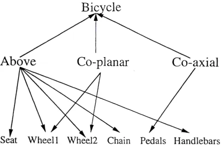
The question now arises as to what exactly do we want to learn. Essentially learning is about providing learned knowledge to solve problems. In this paper we will provide a high-level algorithm which will provide the engine for incremental learning while including accurate tests so that learning with some high degree of assurance is maintained. If we think of a class such as bicycles then we can represent the class by the following feature tree (Figure 1) or, in fact, ea.ch set of features of class bicycle can be represented by (Figure 2), its spatial tree.

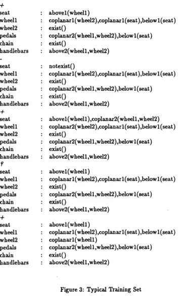
Then a training set that might include positive, negative and/or unknown instances of bicycles might therefore look like (Figure 3). It is this type of training set that SymGb will

finally deal with.

For the purposes of this paper I will now outline the terms that will be used to generate the

SymGb algorithm.

+

?

TsET

e;

Denotes a positive instance of a class, Denotes a negative instance of a class, Denotes an unknown instance of a class, Encompasses the whole training set and

a.re all the elements of each training set and relate to both features and relationships to other features, so seat and exist are both elements of the training set.

Above

Co-planar

Seat Wheel 1 Whee.12 Chain Pedals Handlebars

Figure 1: Feature Tree for Class Ilicyclc

Bicycle

Co-planar

wheell

wheel2

+

seat wheell wheel2 pedals chain handlebars seat wheell wheel2 pedals chain handlebars

+

seat wheell wheel2 pedals chain handlebars

r

seat wheell wheel2 pedals chain handlebars

+

seat wheell wheel2 pedals chain handlebars abovel(wheell)

coplana.rl( wheel2),coplanarl(seat ),belowl( seat) exist()

coplanar2( wheell ,wheel2),belowl( seat) exist()

above2( wheell, wheel2)

notexist()

coplana.rl( wheel2),coplana.rl(seat ),belowl( seat) exist()

coplanar2( wheell, wheel2),belowl( seat) exist()

a.bove2( w heell, w heel2)

a.hovel( wheell ),coplanar2( wheell,wheel2) coplanar2( w heel2) ,coplanar 1 (seat), below 1 (seat) exist()

coplanar2( w heell, w heel2), below 1 (seat) exist()

above2( w heell, wheel2)

abovel( wheell)

coplanarl(wheel2),coplanarl( seat ),belowl( seat) exist()

coplanar2( w heell, w heel2), below 1 (seat) exist()

above2( w heell, w heel2)

a.hovel( wheell)

coplanar 1 ( w heel2) ,coplanar 1 (seat), below 1 (seat) coplanarl(wheell)

coplanar2( w heell, w heel2), below 1 (seat) exist()

above2( wheell,wheel2)

still manually labeled as being either one of positive,negative or of unknown nature. H the set consisted entirely of unknown instances, then the algorithm, as we shall soon see, will make no decisions and no feature tree will result. This point will be tackled later but it is sufficient to plant the seed for further discussion by suggesting that it would suffice to only label the lowest component and that subsequent higher components would be learned. For example only the spoke of a wheel is labeled and then wheell and wheel2 are learned and finally in conjunction with other learned classes, class bicycle is learned.

Learning by example is nothing new and classification is particularly useful for many appli-cations associated with problem solving. Such an example is SOO-PIN [Dance and Ca.elli 1991] where the class learned provides the knowledge base for a Picture Interpretation system. The task of constructing class definitions is called concept learning or induction and the most notable program that provides a platform for determining classes is Winston's program [Winston 1982) which operates on a simple "blocks/world" domain. The basic approach that the program takes, which will be the basis for the SymGb training and classification models, involves the problem of concept formation. Winston's program outlined suggests:

• Begin with a positive instance of the concept and this will become the Null hypothesis or the first description of the concept definition.

• Examine descriptions that are also positive instances of this concept and generalize the concept to include them.

• Examine descriptions that are near misses of this concept and these will be known as negative and unknown instances. Restrict the definition to exclude them.

Although Winston's program provides a basis of the SymGb algorithm, SymGb is an incre-mental learning algorithm.

2.1 Version Space

In conjunction with Winston's program we will use the notion of a Target Space or Version

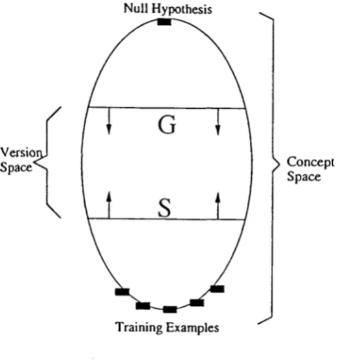
Space [Mitchell 1978] [Cohen and Feigenbaum 1982]. By processing training examples, we want to refine our notion of where the target concept might lie. Our current hypothesis can be represented as a subset of the concept space called the Version Space. So the version space is defined as the largest collection of descriptions that is consistent with all the training examples so far. This version space will consist of two subsets of the concept space. We shall call these subsets, (Mitchell 1978]

• G: The subset that contains the most general descriptions consistent with the training examples seen to date.

• S : The subset that contains the most specific descriptions consistent with the training examples seen to date.

So the version space can be represented by the set of all descriptions that lie between some element of G and some element of S in the partial order of the concept space (See Figure 4).

2.2 Preliminary work with a simple class descriptor

Versio Space

Null Hypothesis

G

Training Examples

Concept Space

Figure 4: Concept and Version Space

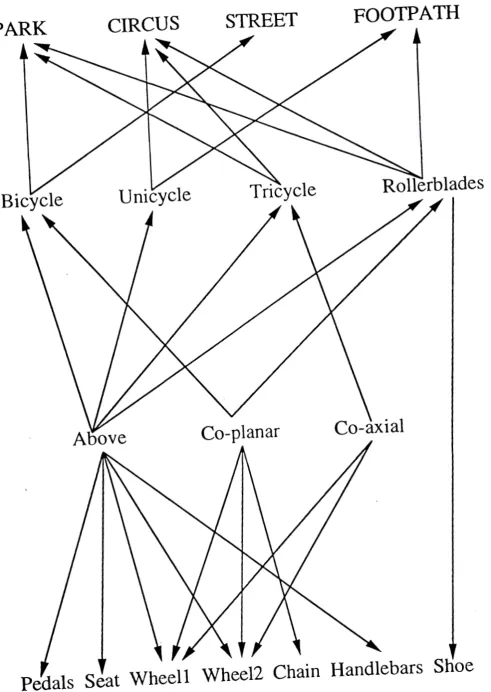
be a simple variant of that proposed by SOO-PIN (Dance and Ca.elli 1991] and the VIMSYS Model (Gupta Weymouth and Jain 1991]. Essentially the feature tree that we will work with is that described by the earlier section (see Figure 1) where we shall assume that this knowledge base exists and we shall now write a simple scene/picture interpreter that will use it. For the purposes of interpreting many classes (ie:scene), the tree will be enlarged to contain several layers of features and relationships. The proposed feature tree will resemble (Figure 5).

In order to identify a high level feature such as a bicycle and hence establish its environment (ie: Park), a series of low level inputs are inserted and a search is carried out on the graph.

2.2.1 A simple algorithm

The search algorithm is simply a greedy algorithm. It must be able to establish paths from lower order features(U nary and Binary) to higher order ones and similarly be able to backtrack to establish connections between features of different levels of the graph, hence the code will be written in Prolog to make use of the inherent backtracking. For example, suppose the input consisted of a set of lower order features such as seat, near, coaxial, handlebars, chain

then each feature in union with all other features would finally make up the solution set and eventually describe the higher order feature class, in this case probably a bicycle or tricycle. Since we will use a Greedy algorithm to decide on possible search paths of our feature tree1 ,

we will need to build lists for probable solutions. When seat is entered as our first feature, the

greedy algorithm will suggest possible solutions lists seat-+ near and seat-+ distant since both

solutions are possible while predicting the next feature. When the next feature is entered, in

1

PARK

CIRCUS

STREET

FOOTPATH

Bicycle

Co-axial

Pedals Seat Wheell Wheel2 Chain Handlebars Shoe

this case near, then the second solution is temporarily halted hut not terminated and the first solution set is enlarged, thus the new possible solution sets are seat - near - coaxial, seat - near - coplanar and seat - distant. If at anytime a feature is entered that promotes the growth of a previously stagnant or relaxed solution set then the list is re-opened and its set enlarged. This means that we can identify a scene with many possible subscenes (ie: a bicycle and unicycle). These lists are grown until no new features exist and the output is a list of lists, each a possible solution. The most probable solution is the list with the most features.

A feature is deemed to be part of a list if it can be matched (ie: it has a relationship to) to each item that already exists in the current solution set. So if we were trying to see if shoe is a feature of one solution set wheel - near - coplanar then we would try to see if shoe is one feature that has a relationship to all of the features that currently exist in this solution set. This is done by backtracking on each feature in the current solution set and shoe. To retain maximal probability of finding a solution, a feature may he inserted and grow more than one solution set. It is also likely that a feature may only be inserted and may not grow the solution set. Similarly if multiple occurrences of a feature is recorded, {ie: many instances of wheels) then multiple solution sets each containing wheels are created, or there may exist in a scene many bicycles, which might he the precondition for a park (ie: Rulepark = Has many bicycles). Finally if we are given a feature that does not belong to any of the current solution sets then a new solution set is created with a single element namely the new feature. Because this work is only a preliminary study for describing the nature of the knowledge base, I will not give this algorithm a name. We can now spell out the algorithm.

Given:

A new feature. One Solution Set.

Algorithm:

while/; do

for ea.ch i E Si do

if

f;

E Si by backtracking then

generalize Si to include /; and enlarge Si else {/;

rt

Si)

temporarily halt this solution set

end for

if there are multiple occurrences off; then create si+l which includes /;

if

f;

rt

anySi then

create si+l which includes

!;

end while

print all solution sets

2.2.2 The data structure

The data structure is a simple one that supports the many solution sets possible. Hence a hashtable with multiple lists is sufficient. Access into the table is 0(1} since an id-number can be associated with each feature and so for all accesses for some n distinct features the total time

spent accessing this table is 0( n ). For each feature

f;

there is a backtracking check involved for the depth of the graph. IT the graph has depth d, then for each feature check, for each solution set which contains possible {n-1} features, the total time spent checking a features validity within a given solution using backtracking would be for i solution sets 0(((n - 1)

*

d)

*

i).

Therefore for n features, the overall time spent adding to or modifying the set of solution sets is E>(n

*

i((n - 1)

*

d)) or O(n3) for a graph of depth n.

2.2.3 Where does learning fit in?

What we would like to do is provide the engine that does the learning and hence creates the feature tree/graph. This would allow a Picture Interpreter to use this knowledge base to classify scenes. Currently the above code uses backtracking within a hardcoded feature graph to establish relationships between features, but unfortunately the graph is hardcoded, therefore there needs to be a learning frontend to this interpreter. As a first step to identifying the role of least generalization within learning it is essential that we look at simple examples that avoid conjuncts, so the training set is a set of positive and negative examples where each example is a set of unary predicates. For the purposes of the proceeding algorithm, we will look at the training set of (Figure 6).

Features in this training set can exist or not exist and whether a set is deemed to be a negative or positive instance depends on the number of features that exist and those that do not exist. The set does not contain instances that are unknown, this is a refinement of the

SymGb algorithm.

2.3

Candidate Elimination Algorithm

Given a representation language, in this case first order predicate calculus, and a set of positive and negative examples that are expressed in this language, then the idea is to compute a concept description that is consistent with all the positive examples and none of the negative examples. The CE (or Candidate Elimination) Algorithm [Charniak 1985] is one such algorithm that can process such rules. Its steps proceed as follows:

1. initialize G to contain the Null description or Null hypothesis, that is that all features are

variables.

2. initialize S to contain the first positive example.

3. Take the next training example:

+

seat True

pedals True

wheell True

wheel2 True

cha.in True

handlebars True

seat True

pedals True

wheell False

wheel2 True

cha.in True

handlebars False

+

seat True

pedals False

wheell True

wheel2 True

cha.in True

handlebars True

seat False

pedals True

wheell True

wheel2 False

cha.in False

handlebars False

+

seat True

pedals True

wheell True

wheel2 True

cha.in True

handlebars True

• H it is a negative example then first remove from S any descriptions that cover this example and then specialize G as little as possible so that the negative example is no longer covered by any of the elements of G. G now contains the most general set of descriptions in the version space that do not cover this example.

4. H Sizeof(G)=Sizeof(S)=l and S

=

G then output G or S as the solution set, halt. 5. H Sizeof(G)=Sizeof(S)=l and S

¢

G then the training set was inconsistent, halt.

6. Else Repeat from step 3 above.

This algorithm can be explained by using the training set described earlier in (Figure 6). In the following table, T and F represent True and False or exist and not exist respectively. The

G and S sets for the data of type (Figure 6) are generalized as follows.

Training Set (G) and (SJ Sets Respectively positive {z1,X2,X3,X4,X5,X6} {T,T,T,T,T,T} negative { X1' X2, T, X4, X5, X6} {T,T,T,T,T,T}

.

{ X1' X2, X3, X4, X5, T}

.

positive { X1' X2, T, X4, X5, X6} {T,x2,T,T,T,T}

.

{ x1, x2, x3, x4, xs, T}

.

negative {T ,x2, T, x4, xs, x6} {T ,x2,T ,T ,T ,T}

.

{T,x2, X3, x4, x 5, T}

.

positive {T,T,T,x4,zs,x6} {T,x2,T,T,T,T}

.

{T,T,x3, x4, zs, T}

.

Table 1 : CE Algorithm

Since G is not a singleton set, more training examples would be required before a solution set can be obtained. Notice that each time a positive example is encountered, the set G or S is generalized by as little as possible, or in this case only by a single feature. Clearly the question that needs to be asked, is what is least general and how does one find the most suitable least generalized update?

2.4 Learning by least generalization

Before deciding on algorithms that use least generalization effectively, it is useful to point out the nature ofleast g~neralization. H we consider a Word to be a literal or term and the symbols V, Vi, W, ... to represent words then we can also define the least generalization as a product in the following category. The objects are therefore words and <1 is a morphism from V to W iff V <1= W and q acts as the identity, c, on all variables not in V. So V is then a least generalization

of {Wi, W2} iff it is a product of W1 and W2. This follows from: [Plotkin 1970]

• If K is a set of words, then Wis a least Generalization of K iff:

1. For every Vin K, W ~ V where ~defines the quasi-ordering.

2. If for every Vin K, W1 ~ V, then W1 ~ W.

• If _{W1 and W2 are any two least generalizations of K then W1 W2 or in terms of the}

We can now apply the following algorithm to show that every non-empty, finite set of words has a lea.st generalization iff any two words in the set are compatible. The algorithm involves simple substitutions of terms in the same places of two words where these terms are not equal or they begin with different function letters or either of these terms may be variables. The algorithm is as follows: [Plotkin 1971]

1. Set

Vi

to each word in K.

2. Find terms ti and t2 to substitute into

Vi

such that ti

#

_{t2 and either} t1 and t2 begin

with different function letters or at lea.st one of them is a variable. t1 and t2 must be substituted into the same place in

Vi

_{and V2.}

3. H the above step cannot be performed then stop and

Vi

is the lea.st generalization of K and

Vi=

V2.

4. Replace instances of t1 and t2 with a distinct variable x.

5. Set£ito{tilx}.

6. Go to step 2.

This algorithm can be best explained with an example. If we wanted to find the lea.st generalization of {P(f(g(y)),u,g(y)),P(h(g(u)),u,g(u))} then:

Set:

Vi

=

P(f(g(y)),u,g(y)) and V2 = P(f(g(u)),u,g(u))

H we substitute ti = y and t2 = u and z as the new variable, then

Vi = P(f(g(z)),u,g(z)) and V2 = P(f(g(z)),u,g(z))

So £i = {ylz} and £2 = {ulz} Note:

Vi= V2 and so

P(f(g(z)),u,g(z)) is the lea.st generalization of K.

It should now be obvious how the generalization steps were performed when working with the training set of (Figure 6).

3

More Supervised Learning - The

Aq

Algorithm

The A q Algorithm (Michalski 1980] is almost equivalent to the repeated application of the

candidate-elimination algorithm. Clever versions of the A9 _{[Michalski 1984] algorithm convert}

4

Plotkins Least Generalization Algorithm

Plotkin's least generalization algorithm [Plotkin 1971] involves using the least generalization algorithm in Section 2.4 to discover the least generalization of a. given set of words where ea.ch substitution of a. new term is induced by a. set of training examples. The algorithm is a continuum of Micha.lski's algorithm (Michalski 1980] a.nd endeavors to find the most specialized bound of a version space. The algorithm is a.s follows:

• Input a set of n positive instances.

• Set G to the Null hypothesis.

• For each instance or training example, apply the lea.st generalization algorithm to gener-alize G.

• Halt when all training examples a.re exhausted.

Since we are only dealing with positive examples, if for each least generalization step only one value is reached, then Plotkin 's algorithm will always find the most specialized expression that covers all of the instances in the training set. The proof for this assertion is outlined in Webb [Webb 1991a]. Some of the problems tha.t both AQ and Plotkin's experience include:

• Their inability to handle negative examples,

• Plotkin 's Algorithm employs a. heuristic search,

• Their inability to handle continuous va.ria.bles a.nd

• Their limitations when handling disjunctive logic.

This means tha.t a new algorithm has to be developed tha.t is far more sophisticated when evaluating negative as well a.s positive examples a.nd an algorithm that is able to handle dis

-junctive as well as con-junctive clauses. Such an option is DLG.

5

DLG

Given:

POS NEG NDL

A set of positive instances tha.t describe the class

A set of negative instances tha.t do not describe the class

A non-disjunctive class description la.ngua.ge where disjuncts will be expressed

DLG Algorithm:

(R = (a. disjunction of disjuncts for the class)) +- false

while there a.re more POS instances

select the next instance form POS

G +- Plot kins( false,instance,ND L)

for each x in POS

end for

G' +- Plotkins( G ,x,ND L)

if G' is not covered in NEG then

G

+-

G'

remove from POS all instances of G

R +- R v G (disjunctive class descriptions)

end while

Examples of run-time performance analysis for DLG can be found in (Webb 1991b], [Webb 1991c] and (Webb and Agar 1991b].

Once again it is important to note tha.t this algorithm does allow for stable incremental learning but although the algorithm allows the induction of non-trivial disjunctive class de-scriptions, which the lea.st generalization algorithm cannot handle, the learning pattern is set by the nature of the POS and NEG sets. Furthermore, DLG is uncompromising in its attempt to prune the feature tree. It makes harsh decisions and so features either exist or are represented by variables. A more relaxed incremental learning will now be demonstrated where evidence is introduced into the lea.st generalization and updates phase.

6

Validity of each training example

will be Bayes' Rule. Bayes' Rule will also be used to supply a. less rigorous update procedure when applying the lea.st generalization to the current class description. Features, both Unary and Binary will only be removed Hf their frequency or probability reach zero. Clearly, if there is evidence for their existence, then they will not be removed from the class description without consideration to previous data items.

6.1 Bayes Rule

Before suggesting Bayes' Rule it is important to introduce some simple probability terminology. Consider an event B in the world, then if the probability of event B is denoted by P(B) then P(B) partitions the sample space S into two disjoint subsets B and -iB. The function P must also satisfy three axioms, namely:

1. P(any event) ~ O;

2. P(S) = 1 and

3. If n events B1 , ••• , Bn E S are collectively exhaustive and mutually exclusive, then the probability that at lea.st one of these events will occur is given by:

n

P(B1 U ··· U Bn)

=

LP(Bi)• (1)

i=l

Now if the sample space S={B,-,B} then for any other event A E S we can say:

P(A)

=

P(A n B) u (An -iB) (2)

and since the union is clearly disjoint:

P(A)

=

P(A

n

B) + P(A

n

-iB)

=

p(AIB)P(B) + P(Al-iB)P(-iB) (3)

by the definition of conditional probability. Now if we were interested in evaluating the condi-tional probability of a single event Bi occurring given that A occurs then:

P(B·IA)

=

P(B,

n

A)

' P(A) (4)

or by the theorem of total probability [Ng and Abramson 1990] we can write:

(5)

The la.st relation is commonly called Bayes' Rule or a posteriori probability.

6.2 Applying Bayes Rule

Bayes Rule can be used to represent two types of conditional structures:

1. The probability of a particular element (ie: existence or non-existence) given that the element has occurred or not occurred in the previous i training sets and

At first glance it is obvious that the occurrence of an element is taken to be quite independent of the other elements that are in the training set. This will not pose a problem for the probability of type 1 but when each training set is a set of conjuncts (ie: a bicycle is a collection of features/elements), what effect will this have on the overall probability of an entire training set.

Probabilities of type 1 can be represented by:

P(B·IB· ) _ P(Bi-1 IBi)P(Bi)

I a-l - Ei':1 P(Bi-1IBi)P(Bi) (6)

where P{Bi) is the probability of event Bi occurring and P(Bi-d is the probability of B occurring in the last i examples, or by example, what is the probability that seat does not exist if I have seen that seat exists in k previous positive examples and seat exists in the last n-k

negative examples. Since seat is a feature in its own right then conditional probability of type 1 is easily catered for.

Conditional probability of type 2 is more subjective. For the purposes of initial trials I have declared all features to be independent when using Bayes rule and so to test the validity of an entire training set, we will apply the conditional probability of type 1 to each feature of the training set while applying the dot product to each probability as they are calculated. For example if the training set is of the form:

wheell wheel2 seat

exist()

exist(),coplanar2( wheell,chain ),belowl( seat) above2( w heell, w heel2)

and it is labeled positive, then the probability that this is a positive training example is given by:

P(Instance is positive

I

Instances before this one)

=

P( wheell exists

I

Instances with wheell before this one) and P{wheel2 exists

I

Instances with wheel2 before this one) and P( seat exists

I

Instances with seat before this one)

The logic may not be entirely sound and is certainly not fully explored however the underlying summations cannot be ignored. The questions that cry out for answers are, Are features of the training set described above independent events and how do their relationships to other features affect their probabilities'? Certainly more research is planned for this area, but for the purposes

of the SymGb algorithm yet to be outlined, the original assumptions will stand. For a further

analysis of Bayes rule refer to [Pearce and Caelli 1992]. One interesting extension of Bayesian Categorization, is an attempt to use it as a similarity measure.

7

Outlining

SymGb

We are now in a position to suggest the SymGb algorithm. Like Plotkin's algorithm, it will use

least generalization to build class descriptions and like DLG will be able to create disjunctive class descriptions, but unlike either ·of its predecessors, SymGb will supply the mechanisms

7 .1 The training set

For the new SymGb algorithm we will make use of the training set outlined in a previous section entitled Learning by examples and is described in (Figure 3). The training set will contain instances of positive, negative and unknown examples of a given class, in this case bicycles. Each instance or example is a set of features which are themselves sets of conjuncts of relationships to other features. The overall training set used contained some 400 examples, in particular 200 positive instances, 150 negative instances and 50 unknown instances. There were positive instances that were equivalent to negative and unknown instances and visa versa. This was done to test various aspects of the generalization and the programs ability to handle spurious and/or conflicting data sets.

7 .2 The

SymGb

Algorithm

At this point we will introduce the Symbolic learning by least generalization and Bayes Rule algorithm or simply put the SymGb algorithm. To illustrate the code at a higher level, let us consider the state diagram of some decisions and actions that must be considered depending on any given state. Note

'+'

implies a positive example, '-' implies a negative example and '?' represents an unknown instance. lg is the application of the least generalization algorithm discussed earlier.

II

state action

Labeled

+

and is first

+

example Null Hypothesis and keep

Labeled

+

and is

+

lg, Label

+

and increase counts of instance Labeled

+

but seen before as

-Bayes predicts - Label - and reduce counts of instance Bayes predicts

+

lg, Label

+

and increase counts of instance Labeled - and is - Label - and decrease counts of instance Labeled - but seen before as

+

Bayes predicts - Label - and reduce counts of instance

Bayes predicts

+

lg, Label

+

and increase counts of instance by 2 Labeled ? but was seen earlier as

+

Repeat steps for

+

instance after Bayes confirmation Labeled ? hut was seen earlier as - Repeat steps for - instance after Bayes confirmation Labeled ? and is ? Add to? list

.

.

Table 2 : Partial State Diagram for SymGb

This algorithm takes as input a training set of type (Figure 3) and unlike most other ing algorithms which involve learning by analogy [Charniak 1985] or explanation-based learn-ing [Charniak 1985], learns rules and trainlearn-ing errors uslearn-ing Bayes Rule 2 instead of rules, decisions and goals being part of the initial input. Furthermore unlike the AQ algorithm [Cohen and Feigenbaum 1982], SymGb does not use any constrained heuristic search hut rather an algorithm that employs a variant of Plotkins least generalization algorithm [Plotkin 1970] and the DLG algorithm [Webb 199la]. The algorithm at the high level is as follows:

2

SymGb Algorithm:

while training set is not empty

remove a.n instance from the training set

if positive instance and first positive instance then First Hypothesis

else Generalize

for the rest of the training set

case (instance) of

(positive): Confirm using Ba.yes

Generalize with current Generalized set3

Increase weights

Remove instance from training set Place on SEEN POSITIVE SET (negative): Confirm using Ba.yes

Generalize with current Generalized set Increase or Decrease weights

H count is zero then replace with variable Remove instance from training set and

Place on SEEN NEGATIVE SET

(unknown): Test using Bayes Classification or refer to SEEN lists Form a. disjunction here and

(end case)

Apply positive or negative steps depending on the evidence Remove instance from training set and

Place on SEEN POSITIVE or NEGATIVE or UNKNOWN SET

Update set of disjunctive class descriptions

end for

Return all seen sets to the training set

end while

Hypothesis testing

The algorithm a.t low level is as follows:

Given:

Tpoa

-Tneg

-Tunknown = TsET

-Positive instance Negative instance Unknown instance

Bayes

threshold= G1iat

Algorithm:

Routine that returns the probability that a given instance is truly a Tpo•

or Tneg as suggested by TsET·

It is also used to validate the existence or non-existence of a particular element of a given Tpo• or Tneg·

Critical value or level of accuracy (ie: 50%)

A disjunction of disjuncts for the class.

/* initialization of all lists

* /

SEENpo• +--Null

SEENneg +--Null SEENunknown +--Null Gtiat +-- Null

while TsET exists and has positive examples, select ((I+-- Tpoa) E TsET)

G +-- lg(G,I)

for each I E TsET

/* Unknown Instance

*/

if (J E SEENunknown)

for each ( ei E J) increase count remove I from SEEN unknown

/*

Positive Instance

* /

if I ....-...+ Tpo• then

/*

First Positive Instance and First Training Example

* /

if ((SEENpo• =Null) and (I¢ SEENne_{9 ))} then

G +--I (Null Hypothesis) SEENpo• +--I

for each ( ei E G) count = 1

/*

Seen before as negative

* /

else if (IE SEENneg) then

/* Confirmed positive

* /

if (Bayes(!)~ threshold) then

remove I from SEEN neg

SEENpoa - I

for ea.ch ( ei E G) increase count

/* Confirmed negative * / else (Bayes(!)< threshold)

/*Is positive */

remove I from SEEN poa SEENneg- I

for ea.ch (ei E (Jn G)) decrease count check-zero

else if (IE SEENpoa) then

G - lg(G,I)

for each ( ei E G) increase count

/* Is positive * /

else ((I¢ SEENne₉)and(I

¢

SEENp011 ) )

G - lg(G,I)

for ea.ch ( ei E (I

n

G)) increase count

SEENpoa - I

/*Negative Instance */ else if Ii--+ Tneg then

/* First Training Instance * /

if (SEENpoa - Null) then

for ea.ch ( ei E (I

n

G)) decrease count check-zero

SEENneg - I

/* Seen before as positive * / else if (IE SEENpoa) then

/* Confirmed negative * /

if (Bayes(!)~ threshold) then

remove I from SEEN poa

for ea.ch ( ei E (I

n

G)) decrease count check-zero

SEENneg- I

/*

Confirmed positive

* /

else

end for

/* Seen before as negative * /

else if (IE SEENneg) then

for each ( ei E (I

n

G)) decrease count check-zero

for each (ei E (In SEENneg)) increase count

/* Is negative * /

else

for each (ei E (In G)) decrease count check-zero

SEENneg +--I

/* Unknown Instance * /

else if I...._... Tun/mown then

/* Seen be/ ore as negative * /

if (IE SEENneg) then

form disjunction and repeat above steps for I...__ Tneg

/*Seen before as positive */

else if (IE SEENpoa) then

form disjunction and repeat above steps for I ...__ Tpos

/* Is unknown * /

else

SE EN unlmown +-- I

/* Disjunctive Class Descriptions * /

Return all SEENp011,SEENnegandSEENunlmown to TsET

end while

/*Hypothesis Testing */

T he algorithm clearly consists of four major tests and actions based on each test. If an instance is matched to an instance that occurred earlier and was earlier described to be unknown, then the counts of all the elements of this example are increased to two and the example is removed from the unknown list. This means that this example whether negative or positive has an increased weight of one because it occurred earlier but was previously unlabeled but is no longer unknown.

I f the example is a positive one then we need to establish the validity of the positive example. Simply stated, Is this truly a positive example? If we have seen no previous positive examples and no negative examples, then this is the first positive example and hence will be Generalized to the Null Hypothesis. This example is placed on the positive instance list and each count for each element in the example is set to 1. If on the other hand this example was seen earlier as a negative example, then the example is tested using Bayes rule for each element of the example and iff it is greater than a particular threshold value (ie: level of confidence) then it is accepted as a positive example and its instance in the negative instance list is removed. This positive example is then least generalized with the current class description G and this instance is added to the positive instance list. If on the other hand the value returned by Bayes rule is less than the threshold value, then the example is added to the negative list and the counts of each element of G that is covered by the example is decreased by one. Finally if the example is clearly a positive example then each of the elements counts in G which are covered by the example are increased by one. Otherwise we increase the counts of each element common to the example and G. In the event of any automatically confirmed positive example {ie: Bayes is not invoked), G is generalized with this new positive instance and the instance is inserted into the positive instance list.

I n the event of a negative example similar tests are performed to validate the authenticity of this instance. If the positive instance list is Null then this is clearly a negative example. Otherwise if this example was seen earlier as a positive example but Bayes rule supports this example as a negative example, then it is removed from the positive instance list and since it is a negative example, each elements count {that is elements common to G and the example) is decreased by one. This instance is placed on the negative list. If Bayes returns a value less than the threshold value then the instance is spurious and so ignored. At first this seems somewhat harsh, but note that the example was originally labeled negative, it was seen on the positive list and Bayes returns a value indicating that it is more likely positive. With too many conflicting values it is better to ignore the example. Finally if the example is labeled negative and is clearly negative since it exists on the negative instance list then we increase the counts of each element in the example and include it to our negative instance list. Otherwise we place this example on the negative instance list and decrease the counts of the elements common to the example and G. If a element reaches a count of zero, then its instance is removed from G entirely. This is in affect a least generalization step itself. In the algorithm above, this check and action is performed after each step where the counts are decreased and is identified by the check-zero function.

F inally, a. la.st clarification, a.n increase or decrease count effectively means a raining or lowering of an elements probability or evidence.

T he above algorithm implies that a call to lg with G (ie: a set of conjuncts that describe the lea.st general class description thus far) and I (ie: the current training set example which is a set of conjunctive unary and binary predicates) as argu~ents, will try to find a. lea.st generalization

G given a. specific training example I. Therefore all calls to lg could be thought of as:

ncalla

L:

lg(G,I)

=

lim V

. G-+S

•=1

where:

G

=

Lea.st generalization,

S = Most specific class description and V

=

Version space.

A notion described by [Mana.go 1987]

Furthermore the function itself is represented by the following algorithm:

/* Null Hypothesis * /

if (G =NULL) then

G +--I

/*Other*/

else

/*Invoke Plotkin's Algorithm */

G' +-- Plotkin( G, I)

/*Not negative

*/

if (G'

¢

SEENne_{9 )} then

G +-- G'

for ea.ch (

e,

E ( G' - ( G

n

G'))) increase count

/*

negative

* /

else

G

Notice that only the counts of the elements that contributed to the lea.st generalization a.re increased. Normally this would result in the counts for those ei 's being set to one. Since I is placed on the

SEENpoa list, the counts for all elements a.re still retained for

N ote that Gliat is the current description of disjuncts for this class and with a bit of care, 'I'

will appear on at most one list (ie: SEEN neg, SEENpo11 , SEENunknownorG).

7.3

Choosing a

threshold

The choice of the threshold value is arbitrary hut since we are essentially dealing with three types of training examples, namely positive, negative or unknown and unknown instances in a perfect setting will eventually be labeled positive or negative, we can think of any instance as begin positive or negative. Since an instance can only be one or the other, the threshold value will be located at 0.50 or 50

7.4 Hypothesis Testing

It is not sufficient for the algorithm to produce just a set of unary and binary predicates that form a set of conjuncts that describe a class. It is also important for the algorithm to estimate within a level of certainty that the final class description is indicative of the training set of examples. We can use the fact that each element of the class description has a count associated with it and it is this count that indicates the relative frequency of each feature with respect to the overall nature of the entire training set of examples, remembering that a class description is made up of a list of disjuncts or features which are themselves described by a list of conjuncts that are essentially unary and binary predicates. To utilize these counts and to formulate hypothesis based on the final class description, we can use tests concerning proportions (Freund and Walpole 1987]. In fact if we set the Null Hypothesis H1 to IJ ~ 0.95 or that our claim is that a particular class description Gi will have feature fxei if at least 953 of the training sets exhibited feature fx then Ho is IJ

<

0.95. It is important to make the subtle difference between elements and features. We can illustrate the nature of both by providing an example. If we had an (J E TsET) of the form:

wheell wheel2 seat

exist()

exist(),coplanar2( wheell ,chain ),belowl( seat) above2(wheell,wheel2)

Then features would be {wheell, wheel2, seat} whereas elements would include {wheell, wheel2, seat, coplanar, exist, above}. Features therefore are always unary, whereas elements may be unary or binary.

With this in mind we would like the final class description to reveal not only the elements and features but with what certainty the the class contains the features and elements. To deal with this problem, I have chosen to use the same approach to features and elements. This may not be the best method but if we can establish that a feature exists as part of a class description with 953 certainty then we can apply the same Null Hypothesis and Hypothesis to each of its elements as if they were a list of disjuncts and not conjuncts. So for the above example one possible Hypothesis for class bicycle could be:

Class bicycle contains features wheell, wheel2 and seat. Some bicycles have feature seat but all (ie: 953) bicycles contain wheell and wheel2. Some bicycles have wheel2 below feature seat but all (ie: 953) of bicycles have the relationship that wheell and wheel2 are coplanar.

7.4.1 Tests concerning proportions

Tests concerning proportions (Freund and Walpole 1987] involve the following steps:

1. Hypothesis

- Ho: B

<

0.95 - Hi: B ~ 0.95

2. Test claim at a

=

0.01

3. Reject Ho if z ~ 2.33 (from z-table scores) where

- for large n (n ~ 100) where n = size of TsET

+ 1

z

= (

x - 2) - nBo

JnBo(l

-80)

where Bo

=

B and the choice between ( +1/2) and (-1/2) depends on whether x (ie: the count associated with each feature and element) is ~or< nB0 •

- for small n (n i 100) where n = size of TsET

x- nB

z= ---;===~

JnB(l - B)

where B =Bo.

4. Else accept Ho.

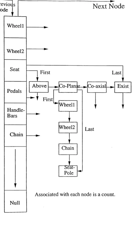
7.5 The Data Structure

The data structure for the positive, negative and unknown instances and G is exactly the same. Each data structure is a linked list of nodes where each node is shown in (Figure 7).

The operations performed on these lists include insertion, deletion and search. Although many data structures are possible, the linked list would be the simplest to manipulate.

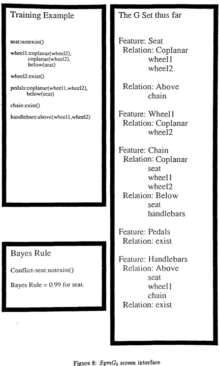
7.6 Running the

SymGb

Algorithm

The interface to the user consists of at most three windows. These windows view the incoming training example, the current status of G and if Bayes rule is called, what instance called it and the outcome of the call. See (Figure 8) for a sample screen. Notice in this example, the training set has instance seat:notexist(), but to date seat has existed in many positive instances of bicycles, so Bayes rule is called to validate the existence or nonexistence of seat. If seat does exist, then the original fact seat:notexist() is ignored in that it plays no part in the least generalization algorithm but its occurrence is sited for possible future use (ie: increase count for this element by -1). This is particularly useful when carrying out hypothesis testing.

7. 7 Time Complexity

Previol s

Node

'f

Next Node

Wheel 1

r---1~

Wheel2

Null

~eat­

Pole

~

Associated with each node is a count.

Training Example

seat:notexist()

wheell:coplanar(wheel2), coplanar(wheel2),

below( scat)

wheel2:exist()

pedals:coplanar(whcel I ,wheel2), below( seal)

chain:exist()

handlebars:above(whecl 1,wheel2)

Bayes Rule

Conflict-seat:notcxist()

Bayes Rule= 0.99 for seat.

The G Set thus far

Feature: Seat

Relation: Coplanar

wheel!

wheel2

Relation: Above

chain

Feature: Wheel 1

Relation: Coplanar

wheel2

Feature: Chain

Relation: Coplanar

seat

wheell

whee12

Relation: Below

seat

handlebars

Feature: Pedals

Relation: exist

Feature: Handlebars

Relation: Above

seat

wheel 1

chain

Relation: exist

number of elements per training example. Note that access to a single item is still 0(1) since we will persist with the ha.shtahle of features being the underlying access-table structure of each node. It is not appropriate to display variations between the various algorithms since the

SymGb is suited to more complex input than any of the other algorithms but SymGb compares

favorably to the DLG algorithm of Webb which is itself on average O(n2_{) [Webb 199la]. Once}

again it is important to note that SymGb exhibits many extra features that DLG does not.

For example, SymGb is invariant to the input and can maintain consistency even if the input

contains unlabeled instances.

8

Learning Higher Level Classes

At first glance the SymGb algorithm seems to be only useful when applied to simple instances

such as bicycles. If we extend our definition of classes by suggesting that all classes are in-dependent or at lea.st that each class can be learned by its own unique data set (ie: training set) consisting of positive, negative and unknown examples, then learning higher level classes is merely applying knowledge of the lower classes that identify the higher class itself. This in turn implies that learning is hierarchical or we learn in a bottom up fashion. This is by no means radical and since each feature or sets of features that identify a class can be learned by its own unique data set, each class description is a problem in itself and so if a higher class is described by a lower or set of lower classes then the implication is that learning is hierarchical. In fact a higher class may only be described by instances covered by its lower level classes and training examples that relate to the higher class directly. If we apply this reasoning to the feature tree/graph of (Figure 5) then we can use a process of unfolding to establish a descrip-tion for class PARK. If all we know of PARK is PARK: has_many(bicycle) (ie: the final class description of class PARK) then this clearly describes the class PARK, hut if we had earlier learned that class bicycle consists of:

bicycle has(wheels)

coplanar( wheell, wheel2) has{seat)

above(seat, wheel2)

then we can unfold class PARK to reveal a more accurate description consisting of:

PARK has_man y (bicycle} where

(bicycle has (wheels)

coplanar( wheell, wheel2) has(seat)

above(seat, wheel2})

Furthermore if we have learned what class coplanar consists of then we get another level of reduction and so forth. Therefore the only limit to the levels of reduction or unfolding that can be applied depends on the amount of knowledge previously learned.

SymGb can now be applied to every level of the feature graph and a final level of reduction

question should add weight to the notion that learning is in fact hierarchical; a statement to be researched at a later stage.

9

Further Research

The whole purpose of this report is to stimulate discussion on the relative advantages of using Ba.yes Rules with Least Generalization. Furthermore, it is not suggested that the algorithm is fault free but rather, new links between the learning phase and the training set may be implied. The time complexity for SymGb needs to be investigated further with various training

sets. SymGb needs to be compared further to DLG with a view to describing the efficiency

differences between the two algorithms, since by its (SymGb) nature the algorithm does not

prune the whole feature graph. The use of Bayes theory is also somewhat predetermined with little or no acknowledgment of other measures, such as Fuzzy logic or Dempster-Shafer theory [Ng and Abramson 1990]. The use of Bayes theory has been chosen because of its appropriateness to Machine Learning. Fuzzy logic and Dempster-Shafer seem to compound the inaccuracy from calculation to calculation and both refer to possibilities of independent hypotheses whereas to determine the accuracy of a particular input example, I need to calculate the probability that the example is correctly labeled given previous training examples. In

short probabilities seem more useful than possibilities. With further investigation outlining the distinct advantages between the three methods being conducted by the department4, I wait

eagerly for the results before attempting my own investigation of the three theories with respect to Ma.chine Learning.

Further investigation also needs to be applied to the use of SymGb with respect to real life

situations. It is somewhat unimportant to learn bicycles and their environment when clearly

Machine Leaming could be better served when applied as a realistic and useful problem solving

technique.

Finally I will investigate the relationship and potential use of SymGb with respect to

Incre-mental Conceptual Clustering [Dechter and Pearl 1987] and [Fisher 1987].

9.1

Knowledge acquisition Via Conceptual Clustering

If we acknowledge that there are two problems associated with conceptual clustering systems namely:

• The actual clustering problem that will involve determining useful subsets of the domain space and

• The problem of characterization that involves classifying objects into useful concepts.

Then the second problem involves learning by examples or the use of the SymGb algorithm.

One possible solution for the first problem is the use of COBWEB [Fisher 1987]. What is further interesting is the evaluation or the representation of these concepts. One possibility is to calculate the probability of attributes using probabilities determined during the learning phase. This is clearly demonstrated during the hypothesis_test phase of the SymGb algorithm.

Therefore from a first glance it seems that SymGb has a place in the overall system of conceptual

clustering and therefore requires further investigation.

9.2 Learning many classes from one training set

If we were to maintain a list of classes, each consisting of a list of disjunctive class descriptions for that class, then for each new instance we can employ the use of a similarity measure such as the Bayesian Categorization Classifier [Cheeseman 1988], to locate the appropriate class description list and the new instance will generalize to it. This allows the maintenance of several class lists. Similarity measures of the form described in Content Addressable Memory Management [Kohonen 1980] are also possible. H these ideas are possible, then what is the nature of negative and unknown examples? Furthermore, how do we deal with convergence of class descriptions (ie: quasi-ordering [Plotkin 1970]) and does this convergence suggest additional useful information about our class descriptions? The major disadvantage we avoid (time wise) is the repeated and independent runtimes of DLG and other learning algorithms to form descriptions for many class .

9.3 Learning Disjunctive Class Descriptions using Version Spaces

Additional work will be carried out on the relative advantages and/or disadvantages of using Version Spaces to providing disjunctive class descriptions. Methods used by NEDDIE and MAGGY (The INSTIL Learning System [Manago 1987]) minus the heuristic selection will be measured against SymGb.

10

Conclusion

The SymGb algorithm provides a number of solutions to the many loopholes that existed in

many of the learning algorithms presented thus far. It has the ability to be invariant to the nature of the training set and therefore has the capacity to alter its generalized set based on contradicting or new training examples. It is more robust (within the limitations of the trails to date performed) than prior algorithms since it handles both negative and positive training examples while still allowing O{N*n) time complexity. The algorithm is by no means complete

but should provide a backbone to a more rigorous algorithm. It seems to have a potential role in the overall problem of conceptual clustering and certainly provides the mechanism for theorem proving using Bayes Rule and hypothesis testing.

The algorithm is used in incremental learning while validating new knowledge against previ-ously learned domain space.

References

[Barr and Feigenbaum 1981] Avron Barr and Edward A. Feigenbaum (Eds) The Handbook of

Artificial Intelligence Vol 1, Pitmann Books LTD, 1981.

[Barr and Feigenbaum 1982] Avron Barr and Edward A. Feigenbaum (Eds) The Handbook of

Artificial Intelligence Vol 2, HeurisTech Press, 1982.

[Charniak 1985] Eugene Charniak and Drew McDermott Introduction to Artificial Intelligence, Addison-Wesley Publishing Company, 1985.

[Cheeseman 1988] P. Cheeseman , et al. AutoClass: A Bayesian Classification System, Pro-ceedings of the fifth International Workshop on Machine Learning, 1988.

[Cohen and Feigenbaum 1982] Paul R. Cohen and Edward A. Feigenbaum The Handbook of

Artificial Intelligence, Volume 3, HeurisTech Press, 1982.

[Dechter and Pearl 1987] Rina Dechter and Judea Pearl Network-Based Heuristics for

Constraint-Satisfaction Problems Artificial vol 34, pp 1-38, 1988.

[Fisher 1987] Douglas H. Fisher Knowledge Acquisition Via Incremental Conceptual Clustering Machine Learning 2: pp 173-190, 1987.

[Dance and Caelli 1991] Sandy Dance and Terry Caelli, A Sym'bolic Object-Oriented Picture

Interpretation Network: SOO-PIN Presented at The International Association for Pattern

Recognition Workshop on Structural and Syntactic Pattern Recognition, August 1992.

[Freund and Walpole 1987] John E. Freund and Ronald E. Walpole Mathematical Statistics, Fourth Edition, Prentice-Hall International Editions, 1987.

[Gupta Weymouth and Ja.in 1991] Amarnath Gupta, Terry E. Weymouth and Ramesh Jain

Semantic Queries with Pictures: The VIMSYS Model Proceedings of VLDB'91, 17th

In-ternational Conference on Very Large Data Bases, Barcelona, Spa.in, Sept 1991.

[Knuth 1973] Donald E. Knuth The Art of Computer Programming Vol 3, Sorting and Search-ing, Addison-Wesley, 1973.

[Kohonen 1980] T. Kohonen Content Addressable Memories, Springer-Verlag, Berlin, Heidel-berg, New York, 1980.

[Manago 1987] M. Manago and J. Blythe Learning Disjunctive Concepts, Lecture Notes in Artificial Intelligence, Vol 347, K. Morik (Ed), Knowledge Representation and Organization in Machine Learning, Springer-Verlag.

[Michalski 1980] R.S. Michalski Pattern Recognition as Rule-Guided Inductive Inference IEEE Transactions on Pattern Recognition and Machine Intelligence, Vol 2, pp 349-361, 1980.

[Michalski 1980] R.S. Michalski, S. Ryszard and R.L. Chilausky Learning by Being Told and

Leaming from Examples: An Experiment Comparison of the Two Methods of Knowledge Acquisition in the Context of Developing an Expert System for Soybean Disease Diagnosis

International Journal of Policy Analysis and Information Systems, Vol 4, No 2, 1980.

[Mitchell 1978) Tom Michael Mitchell Version Spaces: An Approach to Concept Learning, PhD Thesis, Stanford University, Submitted December 1978.

[Neumann and Novak 1984) B. Neumann and H.J. Novak Natural Language Description of

Time-Varying Scenes Report FBI-HH-B-105/84, Hamburg: Fachbereich Informatik, Uni-versity Hamburg, 1984.

[Newell,Allen and Simon 1972] Newell, Allen and H.A. Simon Human Problem Solving Prentice-Hall, 1972.

[Ng and Abramson 1990] Keung-Chi Ng and Bruce Abramson Uncertainty Management in

Ex-pert Systems IEEE Expert, April 1990, pp 29-47, 1990.

[Pearce and Ca.elli 1992] Adrian Pearce and Terry Ca.ell Bayes Rule, Fuzzy Logic and

Dempster-Shafer Yet to be published, Technical Report, CITRI, Melbourne University.

(Plotkin 1970] Gordon D. Plotkin A note on inductive learning, B. Meltzer and D. Mitchle (Eds), Machine Intelligence 5, Edinburgh University Press, Edinburgh, pp. 153-163, 1970.

[Plotkin 1971] Gordon D. Plotkin A further note on inductive generalization, B. Meltzer and D. Mitchie (Eds), Machine Intelligence 6, Edinburgh University Press, Edinburgh, pp.

101-124, 1971.

[Pylyshyn 1982] Z.W. Pylyshyn Literature from Cognitive Psychology Artificial Intelligence, Vol 19, No 3, 1982.

[Schirra,Bosch,Sung and Zimmermann 1987] J.R.J. Schirra, G. Bosch, C.K. Sung and G. Zim-mermann From Image Sequences to Natural Language: A first step toward automatic per-ception and description of motions Applied Artificial Intelligence: 1, pp 287-305, 1987.

[Simon 1969] H.A. Simon The Sciences of the Artificial MIT Press, Cambridge, MA, 1969.

[Small 1990) Melinda Y. Small Cognitive Development Harcourt Brace Jovanovich, 1990.

[Webb 1991a] Geoffery I. Webb, Learning disjunctive class descriptions by least generalization

Technical Report 2/91, Department of Computing and Mathematics, Dekin University, Geelong, 1991.

[Webb 1991b] Geoffery I. Webb, Data Driven Inductive Refinement of Production Rules Aus-tralian Workshop on Knowledge Acquisition for Knowledge-Based Systems, Pokolbin, Au-gust 21-23, pp 44-52, 1991.

[Webb 1991c] Geoffery I. Webb, Einstein- An Interactive Inductive Knowledge Acquisition Tool Technical Report 3/91, Department of Computing and Mathematics, Dekin University, Geelong, 1991.

(Webb and Agar 1991b] Geoffery I. Webb and W.M. Agar The Application of Machine

Leam-ing to a Renal Biopsy Data-Base Technical Report 4/91, Department of Computing and Mathematics, Dekin University, Geelong, 1991.

[Whitehall,Lu and Stepp 1990] B.L. Whitehall, S.C.-Y. Lu and R.E. Stepp CAQ: A Machine

Learning Tool for Engineering Artificial Intelligence in Engineering, 5: pp 189-198, 1990.

[Winston 1982] Patrick Henry Winston Learning New Principles from Precedents and Exercises Artificial Intelligence, Vol 19, No 3, 1982.