7 April 2003
The Effect of Metapopulation Processes on the Spatial Scale
of Adaptation Across an Environmental Gradient
(this article is formally unpublished due to loss of contact with the first author)
Ian R. Wynne1*, Robert J. Wilson2, A.S. Burke3, Fraser Simpson1, Andrew S. Pullin3, Chris D. Thomas2 , James Mallet1
1Galton laboratory, Department of Biology, University College London, 4 Stephenson Way, London NW1 2HE, UK. [email protected], [email protected].
2School of Biology, University of Leeds, Leeds LS2 9JT, UK. [email protected], [email protected].
3School of Biosciences, The University of Birmingham, Edgbaston, Birmingham, B15 2TT, UK. [email protected], [email protected].
* Corresponding author and present address: Department of Population Ecology, Zoological Institute, Copenhagen University, Universitetsparken 15, DK-2100, København Ø; e-mail: [email protected]. Tel: +45 3532 1280. Fax: +45 353 2150.
Keywords: voltinism, adaptation, population genetic structure, connectivity, habitat
networks
ABSTRACT: We show that the butterfly Ariciaagestis (Lycaenidae) is adapted to its thermal environment in via integer changes in the numbers of generations per year (voltinism): it has two generations per year in warm habitats and one generation per year in cool habitats in north Wales (UK). Voltinism is an “adaptive peak” since individuals having an intermediate number of generations per year would fail to survive the winter, and indeed no populations showed both voltinism types in nature. In spite of this general pattern, 11% of populations apparently possess the “wrong” voltinism for their local environment, and population densities were lower in thermally intermediate habitat patches. Population dynamic data and patterns of genetic
differentiation suggest that adaptation occurs at the metapopulation level, with local populations possessing the voltinism type appropriate for the commonest habitat type within each population network. When populations and groups of populations go extinct, they tend to be replaced by colonists from the commonest thermal environment nearby, even if this is the locally incorrect adaptation. Our results illustrate how
Introduction
A critical question in evolutionary biology and ecology is “what is the spatial scale of adaptation?” In evolutionary terms, the answer determines the conditions under which populations are able to diverge (Lenormand 2002), and hence relates to questions about speciation and adaptation, and the ability of range boundaries to expand through successive local adaptations (e.g. Holt 1996; Kirkpatrick and Barton 1997). In an ecological context, local adaptation affects distributions, abundance, population
dynamics and interactions between species (e.g. Singer & Thomas 1996; Tuda and Iwasa 1998; Hanski & Singer 2001).
immigration from populations occupying alternative environments that, for the focal population, carry genes that may be non-adaptive. Effective gene flow can be in the form of ongoing dispersal between extant populations or (re)colonization of empty patches of habitat. The geographical scale over which ecologically relevant traits are differentiated depends on the ratio of the scale of effective dispersal to the scale of the ecological or selective processes involved (Endler 1992; Mallet 2001; Lenormand 2002).
When local populations are subject to frequent extinction within metapopulations (Hanski & Gilpin, 1997), local adaptation is lost and the patch may subsequently be recolonized by migrants from nearby populations. Thus, in metapopulations with high turnover, adaptations to individual patches will be rare, and the traits that predominate are likely to be those associated either with the commonest type of habitat in a network, or the habitat present in the largest patches if these are the least extinction prone and generate most successful colonists (Hanski 1999; Wilson et al.2002).
In this paper we examine the influence of population structure on the distribution and maintenance of allozyme markers and adaptive traits in a butterfly metapopulation distributed across a temperature gradient. At a coarse scale, the temperature changes are very gradual, but at a finer scale temperature is extremely heterogeneous,
gradual environmental change into an integer number of generations. The organism may be required to alter both its life history and responses to environmental cues (photoperiod and temperature sensitivity). Just on the "warm side" of the transition, development must be as fast as possible to ensure two full generations are achieved; just on the "cool side", development must be delayed to ensure exactly one generation. Such differences will be achieved either through local adaptation (populations have one or two generations) or through adaptive polyphenism (developmental response to an environmental trigger).
In this paper we evaluate the spatial scale of voltinism across a heterogeneous
temperature gradient, and investigate whether adaptation to local environments occurs locally or is affected by population turnover in metapopulations.
Study System
In Britain, brown argus butterflies, Aricia Reichenbach (Lycaenidae) occur in populations that have either one (univoltine) or two (bivoltine) generations a year. There is a corresponding difference in adult flight period between these forms: the peak emergence of the univoltine populations falls between the two emergence peaks of the bivoltine populations (Figure 1). Breeding experiments in which univoltine and
consequence of adaptation to climatic conditions, as in other butterflies such as Pieris
brassicae (L.) (Held & Spieth 1999).
Univoltine and bivoltine A. agestis (see taxonomic status, below) populations occur in close proximity in North Wales (Figure 1; Wilson et al. 2002). Here, the habitat of the butterfly (unimproved limestone grassland supporting the larval food plant,
Helianthemum nummularium (L.)) is patchily distributed across a thermal gradient:
warmer in western, low-elevation coastal areas, and cooler in the east at higher
elevation inland sites. Superimposed on this gradient is considerable local variation in thermal microclimate, determined chiefly by aspect, slope and altitude of individual hillsides. These environmental changes occur within very narrow latitudinal limits, so all populations experience approximately the same photoperiods. The fitness of each voltinism will therefore depend on the local thermal environment, and thermally intermediate patches might be expected to support populations with a mixture of voltinisms. But in nature, populations never showed polymorphisms in voltinism (Wilson et al. 2002). Furthermore, colonization and extinction of populations were observed, and small and/or isolated habitat patches were unlikely to be occupied, suggesting that population turnover may be common enough to affect thermal adaptation by A. agestis.
Taxonomic status of north Wales Aricia
Schiffermüller). These species can be mated in captivity and will produce fertile viable offspring (Jarvis, 1966), but the degree to which this occurs in the wild and its success is unknown. In a phylogeographic study of Aricia butterflies in north-western Europe, Aagaard et al. (2002) found two major clades of the mitochondrial gene cytochrome b
(cyt b) separated by 3.3-4.6% sequence divergence. These correspond to the taxa A.
artaxerxes and A. agestis from Scotland/northern Scandinavia and southern
England/southern Scandinavia respectively. However, the univoltine and bivoltine forms in north Wales both appear to belong to a single mitochondrial clade
corresponding to A. agestis, based on six bivoltine (two each from MD, MHW and GT; see Figure 2 for population codes) and six univoltine (two each from GF, LX and PG) individuals (A.S. Burke & I.R. Wynne, unpublished). Three mtDNA haplotypes were found among 12 individuals from north Wales sequenced for cytochrome b. When compared with the known haplotypes within A. agestis and A. artaxerxes, all individuals could be clearly assigned to A. agestis haplotypes of Aagaard et al. (2002: GenBank accession numbers AF408186 to AF408192): Haplotype 1 (MD, GF, LX, PG), Haplotype 2 (MHW) and Haplotype 3 (GT, LX, PG).
Materials and Methods
Distribution Mapping
more if a scrub or woodland barrier was present. With these patch definitions, the closest neighboring patches will typically exchange ~20% of dispersing individuals, but most patches were further apart and should exchange far fewer (Wilson & Thomas 2002). Habitat patch area, aspect (degrees difference from south), slope and altitude were recorded, as well as shelter, H. nummularium cover, bare ground cover and turf height (see Wilson 1999).
The survey was also used to confirm the phenology of A. agestis previously monitored at many of the sites by regular visits and transects (R.W. Whitehead, unpublished data),at a comprehensive list of its populations in north Wales. On the Creuddyn Peninsula (Fig 1), the distribution of A. agestis was mapped, and the date, location and number of A. agestis seen anywhere from 1996-1998 were recorded (Wilson 1999). Numbers of A. agestis were monitored at 24 sites, from May 1996 to July 1998 on standardized weekly transects (Pollard & Yates 1993; Wilson 1999). During summer 1999, weekly transects were walked at a further six populations across mainland north Wales, from the Dulas Valley in the north-west to the Clwydian Hills in the south-east (Figure 1). The weekly transects were used to establish the phenology of bivoltine and univoltine A. agestis (Figure 1b). To determine the voltinism type of all other
Where adults were found, sex and condition (from 4 - mint condition to 1 - completely worn) were recorded, and a transect was walked to give an estimate of population density (see Thomas, 1983a). Populations were assigned to a voltinism type (bivoltine or univoltine) according to the dates and life stages when A. agestis was observed; i.e., the condition and sex ratio of adult butterflies, or the stage of larval development, with reference to the populations where regular transects were carried out. Although there was a small amount of overlap between the end of the first bivoltine adult period and the beginning of the univoltine flight period, and between the end of the univoltine and the beginning of the second generation of the bivoltine flight period (Fig 1b), in practice it was easy to distinguish forms on the basis of adult condition (very old bivoltine and absolutely fresh univoltines in the first overlap period and the reverse in the second overlap period), even on the basis of a single visit.
Thermal Model
From May 1996 to April 1998, temperature was monitored at thirty locations, stratified by aspect and altitude, on the Creuddyn Peninsula (16 on Great Orme’s Head (GO), 14 at Bryn Euryn (BE); Figure 2). Tinytalk dataloggers were placed beneath 5-7 cm tall turf on limestone grassland where H. nummularium grew. Temperature was recorded to the
nearest 0.1°C, every 30 minutes from May to October, and every hour from November to April.
Experimental rearing of univoltine and bivoltine forms showed that larval
unpublished data). Therefore, for each month at each Tinytalk location, we calculated the average number of day degrees > 10°C from the two years’ data (Higley et al. 1986). A monthly thermal model was calculated using the linear regression of cumulative day degrees >10°C against aspect and altitude for all Tinytalk locations which had two years’ data for a particular month (this did not include all locations for all months, because of loss or temporary damage, and because fewer dataloggers were used during winter). For this model, aspect was converted to a linear term by calculating the
difference of site aspect from true south (~185° in north Wales in 1997). As a simple estimate of the length of the Aricia growing season, we used the monthly thermal models to estimate the annual number of day degrees > 10°C at each site, based on its aspect and altitude. This gives a measure of the thermal “development time” available
to A. agestis within each habitat patch.
We used logistic regression (Norusis 1993) to test whether the thermal environment differed significantly between univoltine and bivoltine populations, and to calculate the probability of a population being bivoltine (rather than univoltine).
Connectivity
We estimated likely relative levels of immigration to each habitat patch by calculating connectivity (Si) (Hanski 1994, 1999; Moilanen & Nieminen 2002). Connectivity of focal patch i depends on its distancefrom all other (source) patches (j), the area of each source patch, and the dispersal rate of the species in question. Connectivity for patch i
∑
=
j j
ij i
b
A
d
S
e
α
where α describes how rates of dispersal decline with increasing distance (based on a Cauchy distribution with α = 3; see Shaw 1995; Wilson et al.2002); dij is the distance to
patch i from each source patch j (where i ≠ j); and Aj is the area of each patch j. Source population size scales with patch area, and emigration rate scales with patch area to the power b (set to 0.5, as an approximate description of how butterfly per capita
emigration rate declines with increasing patch area; Thomas & Hanski 1997; Moilanen & Nieminen 2002). For each patch, we calculated Si to all A. agestis populations; i.e., the potential rate of immigration from all other populations. However, we are primarily interested in the relative rates of gene flow (and colonization potential) from bivoltine and univoltine source populations, rather than the overall immigration rate. To estimate this, we calculated the difference between Si calculated i) to all bivoltine populations, and ii) to all univoltine populations that existed during the survey period (connectivity difference). In a network, some habitat patches could be empty in a particular survey period, but might have been occupied in a previous year, at which time populations in them could have contributed to gene flow. Therefore, we also calculated a second term for thermal connectivity difference, based on the thermal characteristics of each habitat patch in the landscape (regardless of whether the habitat was occupied during the survey period). For this second measure, we first calculated whether each patch would be expected to favor bivoltine (“warm patches”) or
voltinism type to habitat thermal characteristics (see results). For each patch, we then subtracted its connectivity to all “cool patches” from its connectivity to all “warm patches.”
Metapopulation modeling
The spatially realistic “incidence function” metapopulation model (IFM; Hanski 1994, 1999) was used to estimate relative persistence times of metapopulations of A. agestis in north Wales. IFM parameters relating extinction rate to patch area, and colonization rate to patch connectivity, were estimated using standard techniques (Moilanen 1999; see appendix material). Fourteen networks containing one or more patches of suitable habitat were defined (Fig 1a), each separated by more than 3 km of unsuitable habitat (Wilson et al. 2002). To estimate relative metapopulation persistence times, 100 IFM simulations of up to 200 generations were iterated for each habitat network. Patch occupancy was set to 100% in the first year of each simulation, in order to compare persistence times of networks that were occupied and unoccupied by A. agestis during the survey.
Population Genetic Structure
Mynydd Marian (MM), Bryn Meiriadog (BM), Bryn Cefn (BC), and Graig Tremeirchion (GT). Localities with univoltine populations were: Graig Fawr (GF), Ochr-y-Foel (OF), Gop Hill (GH), Lixwm (LX), Loggerheads (LOG), Cefn Mawr (CF), Aberduna (AB), Burley Hill Quarry (BHQ), Pistyll Gwyn (PG), Eryrys (EYS), Perthichweru (PW), and Castle Woods (CW). Sample sizes of at least thirty individuals were sought. However, in a few instances this proved difficult or, in the case of very small populations, was deemed undesirable. Samples were heavily male biased to minimize any potential impact on the populations.
Butterflies were snap frozen in liquid nitrogen in the field, and then stored at –80oC. Butterflies were homogenized and prepared for electrophoresis by the methods
described by Wynne and Brookes (1992) using half the thorax and abdomen in 250µl of extraction buffer.
Allozyme variation was assessed using cellulose acetate electrophoresis (Helena Laboratories - see Wynne et al., 1992). A total of 24 enzymes (representing
approximately 31 putative loci) were screened (at least 10 individuals per locus) for polymorphism. These were: adenylate kinase (AK; 2.7.4.3), aconitate hydratase (ACON; EC 4.2.1.3), alanine aminotransferase (GPT; EC 2.6.1.2), alcohol dehydrogenase (ADH; EC 1.1.1.1), diaphorase (DIA; EC 1.6), fumarate hydratase (FUM; EC 4.2.1.2), glucose dehydrogenase (GLDH; EC 1.1.1.47), glutamate-oxaloacetate transaminase (GOT; EC 2.6.1.1), glucose-6-phosphate dehydrogenase (G6PD; EC 1.1.1.49),
-hydroxybutarate dehydrogenase (HBDH; EC 1.1.1.30), isocitrate dehydrogenase (IDH; EC 1.1.1.42), lactate dehydrogenase (LDH; EC 1.1.1.27), malate dehydrogenase (MDH; EC 1.1.1.37), malic enzyme (ME; EC 1.1.1.40), mannose-phosphate isomerase (MPI; EC 5.3.1.8), peptidases (PEP-A and PEP-D, using substrates leucyl-glycine and phenyl-alanine respectively) (PEP; EC 3.4.11), phosphoglucose isomerase (PGI; EC 5.3.1.9), 3-phosphoglycerate dehydrogenase (3PGD: EC ? See Mallet et al. 1993, for details), 6-phosphogluconate dehydrogenase (6PGD; EC 1.1.1.44), phosphoglucomutase (PGM; EC 2.7.5.1), and sorbitol dehydrogenase (SORDH; 1.1.1.14). The running buffers used were 50mM Tris-citrate, pH 7.8 (for ACON, ADH, DIA, αGPD, IDH, 3PGD, 6PGD and
SORDH), 100mM Tris-citrate, pH 8.2 (for AK, GPT, FUM, GOT, G6PDH, HK, HBDH, MDH, and ME) and 25mM Tris-glycine, pH 8.5 (for MPI, PEP-A, PEP-D, PGI and PGM). For most enzymes the duration of the run was 30 minutes at a constant voltage of 200V. The exceptions were PGI and PGM, which were run for 40 minutes (visualized together as a double stain). Staining recipes were used directly or modified from Richardson et al. (1986) and Mallet et al. (1993). Of the loci run, nine were monomorphic (Ak-1, Ak-2,
Fum, Gpt, 6pgd, Dia-1, Ldh-2, Mdh-1, and PepA) and only seven gave scorable
polymorphisms (Pgi, Pgm, Got-2, Mdh-2, Me, G6pd and αGpd).
distance (Slatkin 1993). Slatkin (1993) showed that FST, transformed into Nm (Mˆ in Slatkin's terminology), has a relatively simple relationship with geographical distance under a variety of assumptions about gene flow and population history. A few pairwise
FST values between particularly close and/or well-connected Aricia populations in north
Wales were slightly negative. To avoid losing these data points, and thus biasing the data set, a small quantity of FST (0.01) was added to all pairwise values before
transformation of FST to Nm.
Results
Distribution
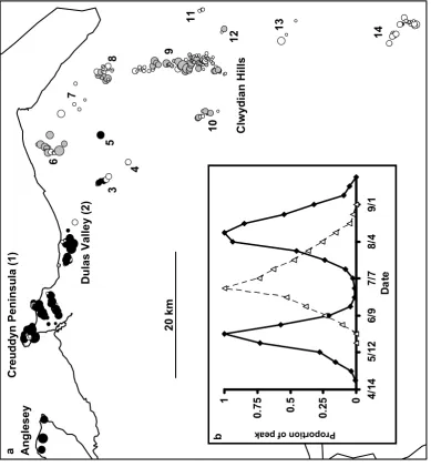
In mainland north Wales, bivoltine populations were found in 87 habitat patches, and univoltine populations in 68 habitat patches in the mainland study region (Figure 1). Population genetic samples were taken from a further three bivoltine populations on the island of Anglesey (Figure 1). The first flight period of bivoltine Aricia stretched from late April to early June, peaking at the end of May; the second flight period extended from mid July to early September, peaking in mid August. The flight period of univoltine Aricia extended from early June to mid August, peaking at the end of June (Figure 1b).
Thermal Model
Monthly day degrees > 10°C were always negatively related to aspect (degrees
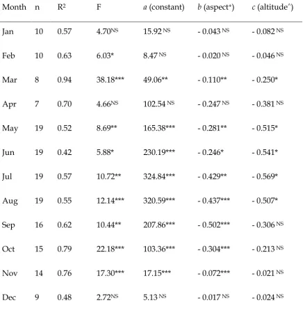
altitude were significant (P < 0.05) for eight and five months respectively. They were rarely significant during the winter months, when fewer dataloggers were used and the number of day degrees > 10°C were much smaller. All monthly equations were used to estimate the annual thermal environment at all habitat patches across north Wales: the non-significant, winter equations have a relatively minor effect on overall estimates, as the constants and coefficients for these months are small (Table 1).
The modeled thermal environment was cooler in sites where univoltine populations occurred than where bivoltine populations occurred. Logistic regression using the thermal model differentiated significantly between bivoltine and univoltine populations (Table 2). Using the thermal model, patches receiving more than 782 day degrees in excess of 10°C per year were expected to support bivoltine populations, and cooler patches were expected to support univoltine populations. Modeled thermal
environment misclassified voltinism at 17 (11%) populations (out of 155). Misclassified populations were located in networks 1, 2, 6, 9 and 10 (Figure 1), so it is unlikely that latitude or proximity to the coast affected results. In particular, the thermal model misclassified five univoltine populations in network 6, and four univoltine populations in network 10: these two habitat networks were at much lower altitudes than other univoltine populations, and had a number of steep, south-facing slopes.
of thermal environment (F1,40 = 6.62, P = 0.01), voltinism (F1,40 = 5.04, P = 0.03), and of their interaction (F1,40 = 7.20, P = 0.01). The interaction term is significant because population density in bivoltine populations decreased at cooler temperatures, whereas the density in univoltine populations increased in cooler environments (Figure 3). Furthermore, density in univoltine populations was positively related to vegetation height (using Spearman’s rank correlation because vegetation height was recorded on a categorical scale; n = 20, rs = 0.62, P = 0.03), again suggesting higher population density in cooler environments (taller vegetation is likely to result in lower day degree
accumulation; Thomas 1983b).
Alternative models using either population connectivity difference or thermal connectivity difference in the logistic regression model explained much more of the observed voltinism pattern than did modeled thermal environment alone (Table 2). Population connectivity difference, calculated to estimate the potential for gene flow from bivoltine and univoltine forms, discriminated between all univoltine and bivoltine populations (Figure 4), such that thermal environment and thermal connectivity
contains the third largest quantity of habitat thermally suitable for the bivoltine form, but is occupied only by the univoltine form.
Metapopulation simulations
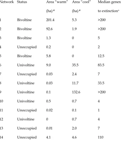
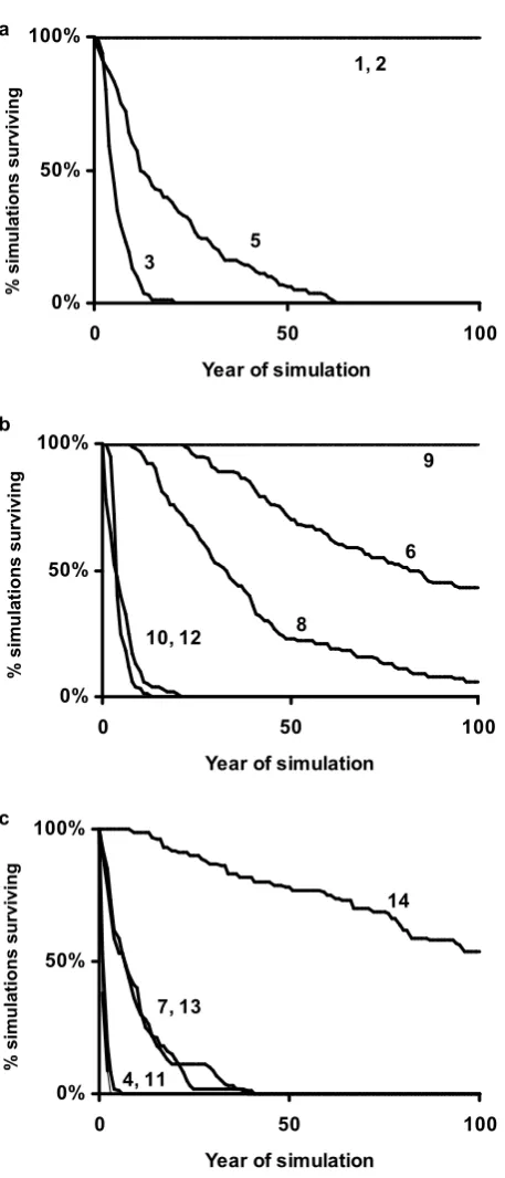
Incidence function modeling predicted that metapopulations in only three habitat networks would persist indefinitely (Table 3, Figure 5). Two of the persistent networks supported bivoltine butterflies, and one persistent network supported univoltine
butterflies (1, 2 and 9 respectively; Fig 1). All other networks occupied by A. agestis had median estimated times to extinction of between 2 and 84 years, shorter than the
modeled time to extinction (median 110 generations) of the most isolated unoccupied network (Table 3). Metapopulation simulations appear to support the conclusion of Wilson et al. (2002), based on habitat network size and configuration, that some small but surviving A. agestis metapopulations may have periodically become extinct, only to be recolonized from the large, persistent metapopulations.
Genetic Variation
Allele frequencies for the seven polymorphic loci are given in the Appendix. Tests for deviations from Hardy-Weinberg equilibrium revealed only 8 significant deviations (P<.05) out of a total of 150 locus x population tests performed. This is similar to the number of significant results expected by chance alone (7.5 expected) and the significant tests were not associated with any particular locus or population (see appendix
Population Genetic Structure in North Wales
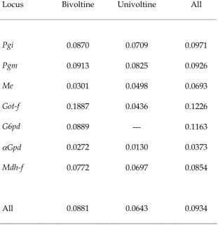
No fixed differences were found between univoltine and bivoltine populations at any of the seven polymorphic loci in north Wales. However there was significant variation of allele frequency among all populations in north Wales (FST = 0.093, P<< 0.001, Table 4). Genetic differentiation within voltinism types was also significant (FST = 0.088, P<< 0.001 and FST = 0.064, P<< 0.001 amongst bivoltine and univoltine populations respectively, Table 4). Pairwise tests between populations revealed that this
differentiation was widespread; only 16 out of 325 comparisons were not significant (at
P< 0.05).
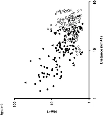
Genetic distance between pairs of populations (14 univoltine, 12 bivoltine) declined with increasing geographic distance (Figure 6). In a three-way Mantel test with 20000 randomized matrices, genetic similarity [log (Nm +1)] was significantly, and negatively, related to geographic distance [log (km+1)] even after controlling for voltinism
(correlation coefficient g = -0.29, P < 0.001), but genetic similarity was unrelated to voltinism after controlling for geographic distance (g = -0.09, P=0.25). Geographic distance is therefore the most important determinant of genetic structure within voltinism types, and has a similar effect in each, but it does not control genetic
differentiation between voltinism types (the slope is weakly in the opposite direction; Figure 6), suggesting that gene flow between voltinism types may be very low.
detectable relationship between within-population heterozygosity and the degree to which populations were connected (Si) to the population network of the same voltinism type (Spearman’s Rank rs = 0.509, P > 0.05 and rs = 0.490, P > 0.05 for bivoltine and univoltine populations respectively).
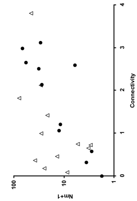
Genetic differentiation of each population from the within-voltinism network mean allele frequency was again calculated using pairwise Nm derived from FST. This measure was significantly correlated with connectivity for bivoltine populations (Spearman’s Rank rs = 0.827, P < 0.01) and the non-significant trend for univoltine populations is in the same direction (rs = 0.469, P > 0.05 ) (Figure 7). Thus, it would appear that drift during colonization events or in small established populations, whilst insufficient to generate detectable losses of heterozygosity, is sufficient to disturb allele frequencies in isolated populations.
Genetic differentiation within the three networks considered persistent by
metapopulation modeling was low but significant: Creuddyn peninsula (network 1; GO, MP, MHW, PYB, LN and BE), FST = .0240 (P << 0.0001); Dulas Valley (network 2; MM, TF and PCB), FST = .043 (P = 0.0446); the Clwydian Hills (network 9; LOG, CF, AB, PG, BHQ, EYS and PW), FST = .0504 (P << 0.0001). Thus population substructure is evident even well-connected networks of local populations. We also sampled three populations (GF, OF and GH) from network 6, which had a predicted metapopulation survival of 43% after 100 generations (Figure 5): differentiation among these
Discussion
The spatial scale of adaptation
Our results indicate that the spatial population dynamics of patchily-distributed species can play a major role in determining patterns of both adaptive and “neutral” genetic variation, at landscape scales that are much larger than expected from dispersal distances achieved by most individuals. Despite the relatively short distances of most individual movements, rare long distance dispersal events have the capacity to
dominate patterns of genetic variation at broad scales, given sufficient turnover of populations and metapopulations.
Aricia agestis appears to show “correct” adaptation to variation in the environment in
89% of the habitat patches in the landscape studied: it converts a smooth, but
heterogeneous, thermal gradient into a binary response of either one or two generations per year. In other words, it achieves alternative adaptive peaks. Yet it is not 100% successful in achieving the “correct” local adaptation in every habitat, and most “local” adaptations almost certainly arise not because of in situ evolution within each patch but because the patch of habitat was colonized by a phenotype that already had appropriate adaptations.
It is apparent that variation in generation number (voltinism) in A. agestis butterflies is an adaptation to the thermal environment, as in many other northern temperate insects. The larvae of both voltinism types have similar minimum temperature
the ‘best’ voltinism strategy will depend on the ‘growing season’ available in a
particular site (measured as day degrees available for development). A bivoltine (two generation per year) strategy will be more successful in warm, low-elevation and/or south-facing conditions and a univoltine (one generation per year) strategy more successful in cool, high-elevation and/or north facing slopes. The reduced density of bivoltine butterflies in relatively cool habitats, and the reduced density of univoltine butterflies in relatively warm habitats suggests that both voltinism types “struggle” in thermally marginal environments.
In heterogeneous conditions, a mixture of the two voltinisms might be expected if (a) life cycle timing was solely a phenotypic response to local environmental conditions or (b) local populations were independently adapted to each local habitat patch. The first of these explanations is not plausible: a variety of microclimates occur within every single habitat patch, and patches differ in thermal environment within each patch network, so we would expect a mixture of voltinism strategies to be observed within most patches and patch networks. The butterflies only ever achieved a single voltinism strategy within each patch and network. Laboratory rearing revealed genetically-based differences in photoperiod responses of univoltine and bivoltine caterpillars
determining whether they enter diapause for the winter, or continue to develop directly to produce a second generation of adult butterflies later in the same summer (A.S.Burke
et al., unpublished). We conclude that genetic differences among populations are
At a patch level, the “wrong” voltinism type in about 11% of local populations, as well as reduced population density in patches with intermediate thermal environments, suggests that local adaptation is incomplete. For example, the north-facing slope of GO (Fig 2) is predicted to be most suitable for a univoltine population on the basis of microclimate, whereas bivoltine butterflies actually occupy the site (at low density). Similarly, butterflies at GF are univoltine (at low density) when bivoltinism is expected. In contrast, all networks of patches contain the voltinism type that is adaptive, based on the amount of each thermal environment that is available across the whole network. The spatial scale and arrangement of habitat patches within the landscape are likely to be important determinants of the traits that predominate (Endler, 1992).
Understanding the scale of adaptation requires consideration of the population dynamics as well as the dispersal behavior of A. agestis.
Metapopulation dynamics
Many species occur as metapopulations whereby entire population systems persist through a dynamic equilibrium between extinction and recolonization (Hanski, 1991; 1999; Thomas and Hanski, 1997). Patterns of patch and network occupancy, observed local and network-level extinctions (Wilson et. al., 2002) and metapopulation
The population genetic structure deduced from allozyme analysis is entirely
consistent with this population dynamic interpretation. Populations peripheral to patch networks are genetically more differentiated from the rest of the network, presumably because of genetic drift and/or founder effects, than central and well-connected
populations. Founder events are likely to contribute to the significant FST values found within each patch network (Taneyhill et al. 2003). However, isolated populations did not have significantly reduced heterozygosity, which initially seems surprising because many of the small and isolated populations in north Wales must have low effective population sizes (Ne ~ < 50). This is probably in part because heterozygosity is relatively insensitive to mild population bottlenecks (Brookes et al. 1997), but is also consistent with metapopulation interpretation: genetic variation within individual populations is not expected to decline over many generations because of the high population turnover rates (Whitlock, 1999). In a conservation context, it is useful to note that areas of high population persistence could be deduced from allozyme data via studies of FST, but not of heterozygosity.
local populations are extinction-prone, the “correct adaptation” within each of the remaining 89% of patches also owes much more to prior colonization by an appropriate phenotype than it does to local adaptation once the population is founded (see Hanski & Singer 2001).
It is likely that a very small fraction of all A. agestis dispersal events is responsible for the network-level patterns of voltinism observed. Colonization of empty patches and networks, and movements between existing populations are distance-dependent. In a mark-release-recapture study, the maximum recorded movement was less than 1km (Wilson & Thomas 2002). Even correcting raw dispersal data because of the finite nature of the mark-release-recapture study area (Wilson & Thomas 2002) produces an estimate of only 0.0004% of butterflies moving the 3.6 km between the habitat networks nearest to one another in the current study. Thus, only tiny fractions of individuals probably move between habitat networks, but those that do appear to exert an important effect on the observed distribution of genotypic and phenotypic variation.
Reservoirs of neutral and adaptive variation
Network-level adaptation would appear to be sufficient to explain patterns of
small networks have a short predicted times to extinction (Figure 5), and A. agestis has been observed to become extinct from two networks in recent years (networks 13, 14; Fig 1). Metapopulations in small but surviving networks probably owe their existence to proximity to the most persistent networks in the landscape, through very rare, long-distance dispersal events (Wilson et al., 2002). Of the persistent systems, the Creuddyn peninsula (network 1) and Dulas Valley (network 2) are clearly dominated by thermal environments suitable for bivoltine A. agestis, whereas the Clwydian Hills (network 9) contain predominantly much cooler habitat, suitable for univoltine forms. Ultimately, the distribution of the adaptive variation in north Wales seems to stem from the
persistence of these key systems and the metapopulation-scale adaptations appropriate within them. Large, well-connected and persistent systems apparently also act as the long-term repository of supposedly neutral allozyme variation within the region, with smaller and more isolated metapopulations containing increasingly divergent allozyme frequencies. In the long run, any new variation that arises within a smaller
metapopulation is likely to be lost, and the empty patch network will ultimately be recolonized from one of the persistent population systems.
In this patchy landscape, extinction-prone, small metapopulations may switch voltinism type from time to time, depending on the origin of recolonists. For example, network 6 is currently populated by univoltine forms, and cool habitats appropriate for univoltine forms are indeed commoner than warm habitats within the network.
models suggest might occur on the order of once every hundred years), the network could be recolonized by either voltinism type: the nearest potential colonists would be in networks 3 and 5, which are both currently bivoltine (Figure 1).
equivalent of the persistent metapopulations within north Wales. Areas of population persistence within generally unstable population systems may dominate patterns of adaptation over surprisingly large areas.
Acknowledgments
We thank Rob Whitehead, James Baker, David Blakeley, Mark Lineham, Rosa
Menéndez, Atte Moilanen for assistance with fieldwork and analysis, and the NERC EDGE program for financial support.
Literature Cited
Aagaard, K., Hindar, K., Pullin, A.S., James, C.H., Hammerstedt, O., Balstad, T. & Hanseen, O. 2002. Phylogenetic relationships in brown argus butterflies
(Lepidoptera: Lycaenidae: Aricia) from north-western Europe. Biological Journal of the Linnean Society 75(1): 27-37.
Barton, N.H. & Whitlock, M.C. 1997. The evolution of metapopulations. In:
Metapopulation Biology: Ecology, Genetics, and Evolution (I. Hanski & M.E. Gilpin Eds) pp. 183-210. Academic Press, San Diego.
Brookes, M.I., Graneau, Y.A., King, P., Mallet, J.L.B., Rose, O.C. & Thomas, C.D. (1997) The genetic consequences of artificial introductions and natural colonizations in the British butterfly Plebejus argus. Conservation Biology 11: 648-661.
relationships in British butterflies I: the effect of mobility and spatial scale. Journal of Animal Ecology 70: 410-425.
Cowley, M. J. R., C.D. Thomas, R.J. Wilson, J.L. León-Cortés, D. Gutiérrez, and C.R. Bulman. 2001b.The density and distribution of British butterflies II: an assessment of mechanisms. Journal of Animal Ecology 70: 426-441.
Endler, J.A. 1992. Genetic heterogeneity and ecology. In: Genes in Ecology (R.J. Berry, T.J. Crawford & G.M. Hewitt Eds). Blackwell, Oxford, pp 534.
Ford, E.B. 1945. Butterflies. Collins, London.
Hanski, I. 1991. Single-species metapopulation dynamics. In: Metapopulation
Dynamics: Empirical and Theoretical Investigations (M. Gilpin & I. Hanski Eds), pp 17 – 38. Academic Press, London.
Hanski, I. 1994. A practical model of metapopulation dynamics. Journal of Animal Ecology 63: 151-162.
Hanski, I. 1999. Metapopulation Ecology. Oxford University Press, Oxford.
Hanski, I. & Gilpin, M.E. (Eds) 1997. Metapopulation Dynamics: Ecology, Genetics and Evolution. Academic Press, London.
Hanski I. & Singer M. C. 2001. Extinction-colonization dynamics and host-plant choice in butterfly metapopulations. American Naturalist 158: 341-353.
Held, C. & Spieth, H.R. 1999. First evidence of pupal diapause in Pieris brassicae L.: the evolution of local adaptedness. Journal of Insect Physiology 45: 587-598.
Hewitt, G. M. 1993 Post-glacial distribution and species substructure: lessons from pollen, insects and hybrid zones. In Evolutionary patterns and processes (eds. D. R. Lees & D. Edwards). The Linnean Society of London Symposium Series 14: 97-123.
Hewitt, G. M. 1996 Some genetic consequences of ice ages, and their role in divergence and speciation. Biological Journal of the Linnean Society 58:247-276.
Hewitt, G. M. 1999 Post-glacial re-colonization of European biota. Biological Journal of the Linnean Society 68:87-112.
Higley, L. G., Pedigo, L. P. & Ostlie, K. R. (1986) DEGDAY: a program for calculating degree-days, and assumptions behind the degree-day approach. Environmental Entomology, 15: 999-1016.
Høegh-Guldberg, O. 1966. Northern European groups of Aricia allous G.-Hb: their variability and relationship to A. agestis (Schiff.) Natura Jutland 13: 9-116.
Jarvis, F.V.L. 1966. The genus Aricia (Lep. Rhopalocera) in Britain. Proc. Transactions of the South London Entomology and Natural History Society 1966: 37-60
Kirkpatrick, M. & Barton N. H. (1997) Evolution of a species’ range. American Naturalist 150: 1-23.
Lenormand, T. (2002) Gene flow and the limits to natural selection. Trends in Ecology and Evolution 17: 183-189.
Mallet, J. (2001) Gene Flow. In: Insect Movement: Mechanisms and Consequences (I.P. Woiwod, D.R. Reynolds & C.D. Thomas Eds), pp 337-360. CABI Publishing, Wallingford, Oxon.
Mallet, J. & Joron, M. 1999. Evolution of diversity in warning color and mimicry: polymorphisms, shifting balance and speciation. Annual Review of Ecology and Systematics 30: 201-233.
Mallet, J., Korman, A., Heckel, D.G. & King, P. 1993. Biochemical genetics of Heliothis
and Helicoverpa (Lepidoptera: Noctuidae) and evidence for a founder event in
Helicoverpa zea. Genetics 86(2): 189-197.
Moilanen, A. 1999. Patch occupancy models of metapopulation dynamics: efficient parameter estimation using implicit statistical inference. Ecology 80: 1031-1043.
Nagelkerke, N.J.D. 1991. A note on a general definition of the coefficient of determination. Biometrika 78: 691-692.
Nei, M. 1972. Genetic distance between populations. American Naturalist, 106: 283-292.
Norusis, M.J. 1993 SPSS for WindowsTM Advanced Statistics Release 6.0. SPSS Inc., Chicago, USA.
Pollard, E. & Yates, T.J. 1993. Monitoring Butterflies for Conservation. Chapman and Hall, London.
Raymond, M & Rousset, F. 1995. GENEPOP (version 1.2): population genetics software for exact tests and ecumenicism. Journal of Heredity 86: 248-249.
Richardson, B.J., Baverstock, P.R. and Adams, M. 1986. Allozyme Electrophoresis. Academic Press, Sydney, pp 410.
Simon, C., Frati, F., Beckenback, A., Crespi., B.J., Lui., H. and Flook, P. 1994. Evolution, weighting and phylogenetic utility of mitochondrial gene sequences and a
compilation of conserved polymerase chain reaction primers. Annals of the Entomological Society of America 87: 651-701.
Singer, M.C. & Thomas, C. D. 1996. Evolutionary responses of a butterfly
metapopulation to human and climate-caused environmental variation. American Naturalist148: S9-S39.
Slatkin, M. & Barton, N.H. 1989. A comparison of three indirect methods of estimating average levels of gene flow. Evolution 43: 1349-1368.
Slatkin, M. 1993. Isolation by distance in equilibriun and nob-equilibrium populations. Evolution 47(1): 264-179.
Taneyhill, D.E., J.B.Mallet , I.Wynne, S.Burke, A.S.Pullin, R.J.Wilson, R.K.Butlin, M.J.Hatcher, B.Shorrocks, and C.D.Thomas. 2003. Estimating rates of gene flow in endemic butterfly races: the effect of metapopulation dynamics. In: Genes in the Environment (R.S.Hails, J.E.Beringer & H.C.J.Godfray, eds). pp. 3-25. Blackwell Science, Oxford.
Thomas, C.D. & Hanski, I. 1997. Butterfly metapopulations. In: Metapopulation Biology: Ecology, Genetics, and Evolution (I. Hanski & M.E. Gilpin Eds) pp. 359 - 386.
Academic Press, San Diego.
Thomas, C.D., Thomas, J.A. & Warren, M.S. 1992. Distributions of occupied and vacant butterfly habitats in fragmented landscapes. Oecologia 92: 563 - 567.
Thomas, J. A. 1983b. The ecology and conservation of Lysandra bellargus (Lepidoptera: Lycaenidae) in Britain. Journal of Applied Ecology 20: 59-83.
Tuda, M & Iwasa, Y. 1998. Evolution of contest competition and its effect on host-parasitoid dynamics. Evolutionary Ecology 12: 855-870.
Wahlberg, N., A. Moilanen, and I. Hanski. 1996. Predicting the occurrence of endangered species in fragmented landscapes. Science 273: 1536 - 1538.
Walsh, S.P., Metzger, D.A., & Higuchi, R. 1991. Chelex 100 as a medium for simple extraction of DNA for PCR-based typing from forensic material. Bio Techniques 10: 506-513.
Weir, B.S. & Cockerham, C.C. 1984. Estimating F-statistics for the analysis of population structure. Evolution, 38: 1358-1370.
Whitlock, M.C. 1992. Temporal fluctuations in demogrphic parametres and the genetic variance among populations. Evolution 46(3): 608-615.
Whitlock, M.C. 1999. Indirect measures of gene flow and migration: FST ≠ 1/(4Nm+1). Heredity 82:117-125.
Wilson, R.J. 1999. The spatiotemporal dynamics of three lepidopteran herbivores of
Wilson, R.J. & Thomas, C.D. 2002. Dispersal and the spatial dynamics of butterfly populations. Pp. 257-278 in: Dispersal Ecology (Ed. J. Bullock, R. Kenward & R. Hails). Blackwell Science, Oxford.
Wilson, R.J., Ellis, S., Baker, J.S., Lineham, M.E., Whitehead, R. & Thomas, C.D. 2002. Large scale patterns of distribution and persistence at the range margins of a butterfly. Ecology 83 (12): 3357-3368.
Wright, S. 1978. Evolution and the genetics of Populations, Vol 4. Variability between and among natural populations. University of Chicago Press, Chicago.
Wynne, I.R. & Brookes, C.P. 1992. A device for producing multiple deep-frozen samples for allozyme electrophoresis. In: Genes in Ecology (R.J. Berry, T.J. Crawford & G.M. Hewitt Eds). Blackwell, Oxford, pp 534.
Table 1. Linear regressions of monthly day degrees > 10°C against aspect and altitude.
Month n R2 F a (constant) b (aspect+) c (altitude^)
Jan 10 0.57 4.70NS 15.92 NS - 0.043 NS - 0.082 NS
Feb 10 0.63 6.03* 8.47 NS - 0.020 NS - 0.046 NS
Mar 8 0.94 38.18*** 49.06** - 0.110** - 0.250*
Apr 7 0.70 4.66NS 102.54 NS - 0.247 NS - 0.381 NS
May 19 0.52 8.69** 165.38*** - 0.281** - 0.515*
Jun 19 0.42 5.88* 230.19*** - 0.246* - 0.541*
Jul 19 0.57 10.72** 324.84*** - 0.429** - 0.569*
Aug 19 0.55 12.14*** 320.59*** - 0.437*** - 0.507*
Sep 16 0.62 10.44** 207.86*** - 0.502*** - 0.306 NS
Oct 15 0.79 22.18*** 103.36*** - 0.304*** - 0.213 NS
Nov 14 0.76 17.30*** 17.15*** - 0.072*** - 0.021 NS
Dec 9 0.48 2.72NS 5.13 NS - 0.017 NS - 0.024 NS
Table 2. Logistic regression models for the voltinism of Aricia agestis populations, based on 1. Modeled thermal environment, 2 Thermal connectivity difference (measured to warm and cool habitats), 3. Population connectivity difference (measured to bivoltine and univoltine butterfly populations).
Model -2LL # R2 Model
Chi2
DF Significance
1. Thermal environment+ 98.76 0.70 113.78 1 <0.001 2. Thermal connectivity
difference^
29.53 0.93 183.01 1 <0.001
3. Population connectivity difference*
0 1 212.54 1 <0.001
Table 3. Occupancy status, thermal environment and modeled time to metapopulation extinction of A. agestis networks in north Wales.
Network Status Area “warm”
(ha) #
Area “cool” (ha) #
Median generations to extinction+
1 Bivoltine 201.4 5.3 >200
2 Bivoltine 92.6 1.9 >200
3 Bivoltine 1.3 0 5
4 Unoccupied 0.2 0 2
5 Bivoltine 5.8 0 12.5
6 Univoltine 9.0 35.5 83.5
7 Unoccupied 0.03 2.4 7
8 Univoltine 0.03 11.7 33.5
9 Univoltine 0.1 132.6 >200
10 Univoltine 0.5 0.7 4
11 Unoccupied 0.02 0.1 1
12 Univoltine 0 0.7 4
13 Unoccupied 0.01 2.0 7
14 Unoccupied 4.1 4.6 110
Table 4. Standardized gene frequency variance FST among univoltine, bivoltine and all populations of Aricia in North Wales for seven polymorphic loci.
Locus Bivoltine Univoltine All
Pgi 0.0870 0.0709 0.0971
Pgm 0.0913 0.0825 0.0926
Me 0.0301 0.0498 0.0693
Got-f 0.1887 0.0436 0.1226
G6pd 0.0889 --- 0.1163
αGpd 0.0272 0.0130 0.0373
Mdh-f 0.0772 0.0697 0.0854
Figure legends
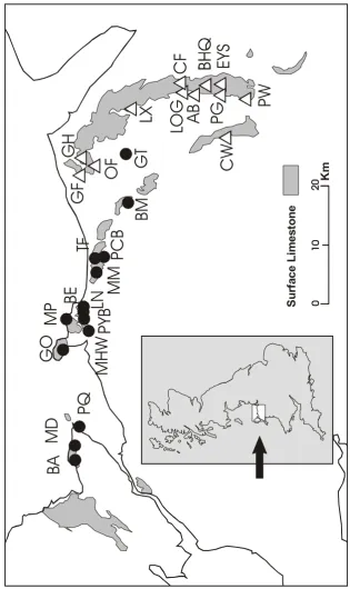
Figure 1.(a)The distribution of bivoltine (black) and univoltine (gray) populations of A.
agestis in north Wales, and of suitable but unoccupied habitat patches (white). Symbol
sizes greatly exaggerate patch size, and are proportional to log patch area. The line shows the north coast of Wales. Place names and numbers are as referred to in the text. (b) Adult emergence patterns for univoltine (n = 4) and bivoltine (n = 24) populations.
Figure 2. Sample localities for univoltine (open triangles) and bivoltine (closed circles)
A. agestis populations in North Wales. Gray areas show the distribution of limestone.
For a key to sample codes see Materials and Methods.
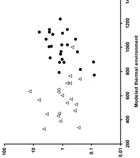
Figure 3. Peak population densityat univoltine (open triangles) and bivoltine (solid circles) populations, plotted against modeled thermal environment (annual modeled day degrees > 10°C).
Figure 4.Modeled thermal environment (annual modeled day degrees > 10°C) against connectivity difference for univoltine (open triangles) and bivoltine (solid circles)
Figure 5. Survival over time of Incidence Function metapopulation simulations for each habitat network. a) networks containing bivoltine A. agestis; b) networks containing univoltine A. agestis ; c) networks unoccupied by A. agestis during the study. Network numbers correspond to those on Figure 1a.
Figure 6. Relationship between genetic similarity (Nm +1) and distance (km+1) in A.
agestis populations in northWales: bivoltine x bivoltine (solid circles), univoltine x
univoltine (solid triangles) and bivoltine x univoltine (open circles) pair wise comparisons. Note the use of Log10 scales.
4
3
u
re
1
.
a Anglesey
Creuddyn Peninsula (1)
Dulas Valley (2)
3
4
5
6
7
8 9
10
11
12
13
14
Clwydian Hills
20 km
b
0
0
.2
5
0
.5
0
.7
5
1 4/1
4
5
/1
2
6
/9
7
/7
8
/4
9
/1
D
a
te
4
4
u
re
2
.
P
Q
M
D
B
A
G
O
M
P
M
H
W
P
Y
BL
N
B
E
TF
P
C
B
M
M
B
M
G
T
G
F
O
F
G
H
LX
C
F
A
B
LO
G
E
Y
S
P
G
C
W
P
W
0000
1
0
1
0
1
0
1
0
2
0
2
0
2
0
2
0 K
m
S
u
rf
a
c
e
L
im
e
s
to
n
4
5
u
re
3
.
0
.0
1
0
.1
1
1
0
1
0
0 2
0
0
4
0
0
6
0
0
8
0
0
1
0
0
0
1
2
0
0
1
4
0
0
M
o
d
e
le
d
t
h
e
rm
a
l
e
n
v
ir
o
n
m
e
n
t
4
6
u
re
4
.
0
4
0
0
8
0
0
1
2
0
0
1
6
0
0 -2
0
-1
0
0
1
0
2
0
C
o
n
n
e
c
ti
v
it
y
d
if
fe
re
n
c
e
Figure 5.
a
0% 50% 100%
0 50 100
Year of simulation
%
s
im
u
la
ti
o
n
s
s
u
rv
iv
in
g
1, 2
5 3
b
0% 50% 100%
0 50 100
Year of simulation
%
s
im
u
la
ti
o
n
s
s
u
rv
iv
in
g 9
6
8 10, 12
c
0% 50% 100%
0 50 100
Year of simulation
%
s
im
u
la
ti
o
n
s
s
u
rv
iv
in
g
14
7, 13
4
8
u
re
6
. 1
1
0
1
0
0
1
1
0
1
0
0
D
is
ta
n
c
e
(
k
m
+
1
)
4
9
u
re
7
. 1
1
0
1
0
0
0
1
2
3
4
C
o
n
n
e
c
ti
v
it
y
5 0 ct ro n ic e n h a n ce m e n ts . p e n d ix m a te ri a l: A ll o z y m e a ll e le f re q u e n ci e s el e fr eq u en ci es f o r ei g h t p o ly m o rp h ic l o ci i n ( A ) b iv o lt in e an d ( B ) u n iv o lt in e p o p u la ti o n s o f A ri ci a . A ls o p ro v id ed a re t h e m b er o f in d iv id u al s sa m p le d ( N ), o b se rv ed ( O b s. ), E x p ec te d ( E x p .) a n d m ea n H et er o zy g o si ty ( * in d ic at es a s ig n if ic an t d ev ia ti o n m H ar d y -W ei n b er g e x p ec ta ti o n s, P < 0 .0 5) . _ _ _ _ _ _ _ _ _ _ _ _ _ _ _ _ _ _ _ _ _ _ _ _ _ _ _ _ _ _ _ _ _ _ _ _ _ _ _ _ _ _ _ _ _ _ _ _ _ _ _ _ _ _ _ _ _ _ _ _ _ _ _ _ _ _ _ _ _ _ _ _ _ _ _ _ _ _ _ _ _ _ _ _ _ _ _ _ _ _ _ _ _ _ _ _ _ _ _ _ _ _ _ _ _ _ _ _ _ _ _ _ _ _ _ _ _ _ M D B A P Q G O M P M H W P Y B L N B E M M T F P C B B M G T _ _ _ _ _ _ _ _ _ _ _ _ _ _ _ _ _ _ _ _ _ _ _ _ _ _ _ _ _ _ _ _ _ _ _ _ _ _ _ _ _ _ _ _ _ _ _ _ _ _ _ _ _ _ _ _ _ _ _ _ _ _ _ _ _ _ _ _ _ _ _ _ _ _ _ _ _ _ _ _ _ _ _ _ _ _ _ _ _ _ _ _ _ _ _ _ _ _ _ _ _ _ _ _ _ _ _ _ _ _ _ _ _ _ _ _ _ _
i N)
5 0 3 0 3 0 5 2 5 0 5 0 5 9 5 0 4 9 2 5 5 0 4 2 5 1 2 1 A . 3 0 0 . 2 6 7 . 3 5 0 . 5 1 9 . 5 3 0 . 3 9 0 . 3 9 8 . 5 6 0 . 4 0 8 . 1 8 0 . 2 4 0 . 1 1 9 . 2 4 5 . 0 4 8 B . 2 4 0 . 1 8 3 . 3 5 0 . 2 4 0 . 1 5 0 . 1 4 0 . 3 1 4 . 2 0 0 . 2 1 4 . 2 0 0 . 2 2 0 . 2 8 6 . 0 1 0 . 3 1 0 C . 0 1 0 . 0 5 0 . 0 6 7 . 0 7 7 . 1 1 0 . 3 1 0 . 1 2 7 . 0 7 0 . 2 1 4 . 5 0 0 . 3 5 0 . 3 6 9 . 2 0 6 . 5 4 8 D . 4 5 0 . 5 0 0 . 2 3 3 . 1 6 3 . 2 1 0 . 1 6 0 . 1 6 1 . 1 7 0 . 1 6 3 . 1 2 0 . 1 9 0 . 2 2 6 . 5 3 9 . 0 9 5
E : bs
. . 5 4 0 . 6 0 0 . 6 3 3 . 7 5 0 . 4 4 0 * . 6 2 0 . 8 3 1 . 6 8 0 . 7 3 5 . 6 8 0 . 7 8 0 . 7 6 2 . 6 4 7 . 5 7 1 x p . . 6 4 0 . 6 4 3 . 6 9 6 . 6 4 0 . 6 4 0 . 7 0 7 . 7 0 1 . 6 1 3 . 7 1 5 . 6 6 3 . 7 3 5 . 7 1 7 . 6 0 7 . 5 9 3
m N)
5 0 3 0 3 0 5 2 5 0 5 0 5 9 5 0 4 9 2 5 5 0 4 2 5 1 2 1 A . 2 0 0 . 2 6 7 . 2 3 3 . 0 2 0 . 0 1 7 . 0 1 0 . 0 8 0 . 0 9 0 . 0 8 3 B . 6 5 0 . 6 8 3 . 6 6 7 . 7 6 9 . 5 3 0 . 4 1 0 . 5 4 2 . 5 8 0 . 4 3 9 . 5 2 0 . 5 8 0 . 4 8 8 . 9 1 2 . 4 0 5 C . 1 5 0 . 0 5 0 . 1 0 0 . 1 7 3 . 3 2 0 . 5 1 0 . 3 4 7 . 2 7 0 . 3 9 8 . 4 0 0 . 3 2 0 . 3 6 9 . 5 9 5 D . 0 5 8 . 1 3 0 . 0 8 0 . 0 9 3 . 1 5 0 . 1 5 3 . 0 1 0 . 0 6 0 . 0 8 8
: bs
. . 3 8 0 * . 5 6 7 . 4 6 7 . 3 8 5 . 5 8 0 . 4 8 0 . 7 1 2 * . 6 0 0 . 5 7 1 . 6 0 0 . 5 6 0 . 5 2 4 * . 1 7 6 . 4 2 9 x p . . 5 1 5 . 4 5 9 . 4 9 1 . 3 7 5 . 5 9 9 . 5 6 5 . 5 7 6 . 5 6 8 . 6 2 6 . 5 6 3 . 5 5 3 . 6 1 5 . 1 6 1 . 4 8 2 N ) 5 0 3 0 3 0 5 1 5 0 4 9 5 1 5 0 4 3 2 5 5 0 4 2 5 1 2 1 A . 4 6 0 . 3 1 7 . 5 3 3 . 6 7 6 . 6 7 0 . 5 3 1 . 6 5 7 . 5 9 0 . 6 2 8 . 7 0 0 . 5 8 0 * . 5 6 0 . 6 6 7 . 4 5 2 B . 5 4 0 . 6 8 3 . 4 6 7 . 3 2 4 . 3 3 0 . 4 6 9 . 3 4 3 . 4 1 0 . 3 7 2 . 3 0 0 . 4 2 0 . 4 4 0 . 3 3 3 . 5 4 8
: bs
5 2 _ _ _ _ _ _ _ _ _ _ _ _ _ _ _ _ _ _ _ _ _ _ _ _ _ _ _ _ _ _ _ _ _ _ _ _ _ _ _ _ _ _ _ _ _ _ _ _ _ _ _ _ _ _ _ _ _ _ _ _ _ _ _ _ _ _ _ _ _ _ _ _ _ _ _ _ _ _ _ _ _ _ _ _ _ _ _ _ _ _ _ _ _ _ _ _ _ _ _ _ G F O F G H L X L O G C F A B P G B H Q E Y S C W P W _ _ _ _ _ _ _ _ _ _ _ _ _ _ _ _ _ _ _ _ _ _ _ _ _ _ _ _ _ _ _ _ _ _ _ _ _ _ _ _ _ _ _ _ _ _ _ _ _ _ _ _ _ _ _ _ _ _ _ _ _ _ _ _ _ _ _ _ _ _ _ _ _ _ _ _ _ _ _ _ _ _ _ _ _ _ _ _ _ _ _ _ _ _ _ _ _ _ _ _
i N)
4 1 5 4 5 0 3 0 2 0 5 0 5 0 6 0 5 0 5 0 1 8 5 0 A . 5 7 3 . 2 4 1 . 4 2 0 . 3 1 7 . 1 5 0 . 1 8 0 . 2 2 0 . 1 8 3 . 1 8 0 . 1 7 0 . 1 9 4 . 0 5 0 B . 2 2 0 . 3 7 0 . 2 8 0 . 1 8 3 . 5 5 0 . 3 7 0 . 3 5 0 . 5 5 0 . 4 1 0 . 5 8 0 . 3 8 9 . 5 7 0 C . 0 2 4 . 0 3 0 . 1 6 7 . 0 5 0 . 1 1 0 . 0 8 3 . 0 8 0 . 1 3 0 . 4 1 7 . 1 3 0 D . 1 8 3 . 3 8 9 . 2 7 0 . 3 3 3 . 2 5 0 . 4 5 0 . 3 2 0 . 1 8 3 . 3 3 0 . 1 2 0 . 2 5 0
E : bs
. . 6 3 4 . 6 3 0 . 6 2 0 . 7 3 3 . 7 5 0 . 6 2 0 . 7 0 0 . 6 3 3 . 7 0 0 . 6 4 0 . 6 1 1 . 6 6 0 x p . . 5 8 9 . 6 5 4 . 6 7 1 . 7 2 7 . 6 1 0 . 6 2 8 . 7 1 5 . 6 2 3 . 6 8 4 . 6 0 3 . 6 3 7 . 5 9 3
m N)
4 2 5 4 5 0 3 0 2 0 5 0 5 0 6 0 5 0 5 0 1 8 5 0 A . 0 1 2 . 0 7 4 . 1 4 0 . 0 3 3 . 1 7 5 . 1 6 0 . 0 7 5 . 0 3 0 . 0 7 0 . 1 1 1 . 0 2 0 B . 4 4 0 . 4 9 1 . 4 1 0 . 5 8 3 . 5 2 5 . 5 8 0 . 4 7 0 . 5 7 5 . 6 0 0 . 5 7 0 . 8 0 6 . 1 5 0 C . 4 4 0 . 4 3 5 . 4 4 0 . 3 6 7 . 3 0 0 . 2 3 0 . 4 4 0 . 3 0 0 . 3 0 0 . 3 2 0 . 0 8 3 . 8 3 0 D . 1 0 7 . 0 1 0 . 0 1 7 . 0 3 0 . 0 9 0 . 0 5 0 . 0 7 0 . 0 4 0
: bs
. . 5 4 8 . 4 0 7 . 6 2 0 . 5 0 0 . 6 0 0 . 5 8 0 . 6 0 0 . 5 6 7 . 3 8 0 * . 5 4 0 . 3 3 3 . 3 0 0 x p . . 6 0 0 . 5 6 4 . 6 1 9 . 5 2 4 . 6 0 4 . 5 8 4 . 5 7 7 . 5 7 1 . 5 4 4 . 5 6 6 . 3 3 2 . 2 8 8 N ) 4 2 5 4 4 9 2 9 1 9 5 0 5 0 5 9 5 0 5 0 1 8 5 0 A . 2 5 0 . 2 6 9 . 3 6 7 . 5 1 7 . 4 2 1 . 3 8 0 . 4 9 0 . 4 2 4 . 4 0 0 . 4 0 0 . 1 6 7 . 6 5 0 B . 7 5 0 . 7 3 1 . 6 3 3 . 4 8 3 . 5 7 9 . 6 2 0 . 5 1 0 . 5 7 6 . 6 0 0 . 6 0 0 . 8 3 3 . 3 5 0
: bs
. . 5 0 0 * . 3 8 9 . 5 7 1 . 4 8 3 . 5 2 6 . 4 8 0 . 5 4 0 . 5 0 8 . 5 2 0 . 5 2 0 . 3 3 3 . 3 8 0 x p . . 3 7 5 . 3 9 3 . 4 6 5 . 4 9 9 . 4 8 8 . 4 7 1 . 5 0 0 . 4 8 8 . 4 8 0 . 4 8 0 . 2 7 8 . 4 5 5 t -f N ) 4 2 5 3 5 0 3 0 2 0 5 0 4 9 6 0 4 9 5 0 1 8 5 0 A B . 8 1 0 . 7 1 7 . 9 1 0 . 7 3 3 . 6 2 5 . 6 1 0 . 8 1 6 . 6 5 0 . 6 1 2 . 7 1 0 . 5 8 3 . 5 8 0 C . 1 9 0 . 2 8 3 . 0 9 0 . 2 6 7 . 3 7 5 . 3 9 0 . 1 8 4 . 3 5 0 . 3 8 8 . 2 9 0 . 4 1 7 . 4 2 0
: bs
Appendix material: Metapopulation modeling methods
Incidence function model (IFM)
The Incidence Function Model (Hanski 1994, 1999) is a spatially realistic
metapopulation model, based on the assumptions that population extinction
rate is negatively related to habitat patch area, and that patch colonization rate is positively related to patch connectivity.
Connectivity for patch i (Si)is defined as Si = ∑ exp (-αdij) Ajb where α is the
slope of the dispersal kernel (the cumulative proportion of per generation
dispersal over distance d km or greater corresponds to exp-αd for a negative
exponential dispersal kernel); dijis the distance to patch i from each occupied
source patch j (where i≠j); and Aj is the area (ha) of each patch j. Source patch
emigration rate scales with patch area to the power b.
IFM is based on the equation (Hanski 1994, 1999):
i i
i i
S A
x ey J
J
ln 2 ln ) ln( 1
ln =− + +
−
where Ji is the incidence or long-term probability of occupancy of patch i, Ai
and Siare respectively the area and connectivity of patch i,and e, y and x are parameters of extinction and colonization. The annual colonization
probability of patch i is Ci = Si2 / (Si2+ y2) ; and annual extinction probability,
Ei = (e / Aix) (1-Ci). In the model, patches with high connectivity (Si) are more
large area (Ai) are less likely to go extinct than small patches. Patches with
high annual colonization probability are more likely than isolated patches to
be “rescued” from extinction, and extinction rate is multiplied by 1-Ci to take
account of the rescue effect. The risk of extinction is unity where minimum patch area A0 = e1/x. Thus, A0, e and x scale the relationship between patch
area and extinction, and y determines the relationship between connectivity
and colonization probability.
We estimated e, y, and x using 1997 occupancy data for the Creuddyn
Peninsula, where we were confident that most if not all habitat patches had
been identified (n=89), and where the distribution of limestone grassland has
been relatively stable for the last 100 years (9% decline, Cowley et al. 1999).
We used the method described in software available from the website at http://www.helsinki.fi/science/metapop/ (see Hanski 1994, 1999, Moilanen
1999). For A. agestis we used a negative exponential dispersal kernel of α=2,
as has been used for species with similar dispersal rates determined by mark-release-recapture studies (e.g., Hanski 1994, Wahlberg et al. 1996, Wilson and
Thomas 2002). Per capita emigration rate tends to decline with increasing
patch area (Thomas and Hanski 1997, Hanski et al. 2000), and parameter b
was set to 0.5 (A. Moilanen personal communication). Minimum patch area
(A0) was estimated from field observations to be 0.05 ha. The probability of
colonization from outside the network was set to zero, because the nearest
Regional stochasticity was set to zero, based on data which showed
asynchronous dynamics of A. agestis in patches less than 1 km apart (Wilson
1999). The Monte Carlo Markov Chain (MCMC) method was used for the
final parameter estimation, with 1000 function evaluations in initiation and 4000 function evaluations in estimation (Moilanen 1999).
Incidence function parameters estimated from the distribution of occupied
and vacant habitat patches in the Creuddyn Peninsula were: x = 0.604 (95%
C.I.s 0.306-1.314), ey2 = 0.329 (95% C.I.s 0.107-0.466), e = 0.164, y = 1.418. To
estimate metapopulation persistence, we ran 100 IFM simulations of up to 200
generations for each habitat network, using estimated values of e, y, and x,
and the above values for α, b and A0. We set 100% patch occupancy in the
first year of each simulation, and zero regional stochasticity, so estimated