University of South Carolina
Scholar Commons
Theses and Dissertations
2016
Chebyshev Inversion of the Radon Transform
Jared Cameron Szi
University of South CarolinaFollow this and additional works at:https://scholarcommons.sc.edu/etd
Part of theMathematics Commons
This Open Access Thesis is brought to you by Scholar Commons. It has been accepted for inclusion in Theses and Dissertations by an authorized administrator of Scholar Commons. For more information, please [email protected].
Recommended Citation
Chebyshev Inversion of the Radon Transform
by
Jared Cameron Szi
Bachelor of Arts
University of California, Davis 2014
Submitted in Partial Fulfillment of the Requirements
for the Degree of Master of Arts in
Mathematics
College of Arts and Sciences
University of South Carolina
2016
Accepted by:
Pencho Petrushev, Director of Thesis
Joshua Cooper, Reader
c
Copyright by Jared Cameron Szi, 2016
Abstract
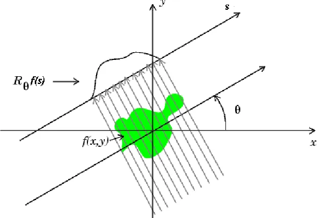
In its two-dimensional form, the Radon transform of an image (function) is a
col-lection of projections of the image which are parameterized by a set of angles (from
the positive x-axis) and distances from the origin. Computational methods of the
Radon transform are important in many image processing and computer vision
prob-lems, such as pattern recognition and the reconstruction of medical images. However,
computability requires the construction of a discrete analog to the Radon transform,
along with discrete alternatives for its inversion. In this paper, we present discrete
analogs using classical methods of Chebyshev polynomial reconstruction, along with
a new computational method which makes use of sub-exponentially localized frames
comprised of Chebyshev polynomials. This new method leads directly to a potential
Table of Contents
Abstract . . . iii
List of Figures . . . vi
Chapter 1 Introduction . . . 1
Chapter 2 The Continuous Radon Transform. . . 5
2.1 Classical Chebyshev Inversion Formula . . . 5
2.2 Classical Fourier Inversion Formula . . . 12
Chapter 3 The Discrete Radon Transform . . . 18
3.1 Discrete Analog of Classical Chebyshev Inversion Formula . . . 18
3.2 Data Acquisition Algorithms for the Discrete Radon Transform . . . 20
Chapter 4 Sub-Exponential Localization Properties of Needlets 29 Chapter 5 Ridgelet Inversion of the Radon Transform . . . 40
5.1 Orthogonal Expansion using Chebyshev Polynomials . . . 40
5.2 Construction and Computation of the Ridgelet Inversion Formula . . 45
Bibliography . . . 52
Appendix A Source Code . . . 54
A.2 Discrete Line Integral: Algorithm 2 . . . 58
A.3 Discrete Radon Transform . . . 60
List of Figures
Figure 1.1 The Radon Transform . . . 2
Figure 1.2 Sinogram . . . 3
Figure 3.1 8×8 Image Region . . . 21
Figure 3.2 256×256 Shepp-Logan Phantom Head . . . 22
Figure 3.3 Image Representation on an Image Region . . . 22
Figure 3.4 Pixel Intersection . . . 23
Figure 3.5 Length of Pixel Intersection . . . 24
Figure 3.6 Various Types of Pixel Cuttings . . . 26
Figure 3.7 Algorithm A.1: Image Reconstruction . . . 26
Figure 3.8 Algorithm A.2: Image Reconstruction . . . 27
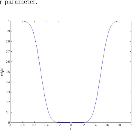
Figure 5.1 Plot of φ4(t) . . . 42
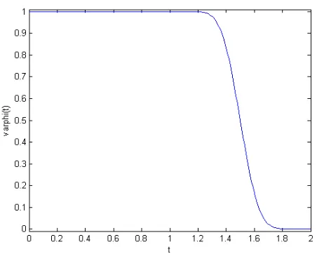
Figure 5.2 Plot of Cutoff Functionϕ(t) . . . 43
Figure 5.3 Localization of Kernel ΦM . . . 44
Figure 5.4 Visualization of Smoothness Issues oftϕ(t) . . . 46
Figure 5.5 Visualization of Ridgeletsψν . . . 47
Figure 5.6 Plot of ω(t) . . . 50
Chapter 1
Introduction
An integral transform is any transform T of the form
(T f) (u) = Z t2
t1
K(t, u)f(t)dt.
It is a transform in the sense that the input of the transform is a functionf, and the
output is yet another function T f. While there are many integral transforms that
have useful applications, one that has remained of primary interest (particularly in
the field of tomography) is the Radon transform.
Let f ∈ C01(R2), the space of compactly supported, continuously differentiable
functions. The Radon transform of f is defined to be a function on the space of
straight lines inR2,
Rf(L) = Z
L
f(x)dx. (1.1)
Any straight line L inR2 can be parameterized in the form
L= (scosφ+tsinφ,−ssinφ+tcosφ), s∈R,
wheretis the distance ofLfrom the origin and φis angle betweenLand the positive
x-axis. Using the following notation,
θ= (cosφ,sinφ), θ⊥= (−sinφ,cosφ), (1.2)
it follows that (1.1) can be expressed as
Rθf(s) =Rf(θ, s) =
Z
R
As we’ve alluded to, the Radon transform is used in a variety of applications in
the field of tomography, which is concerned with the reconstruction of an image from
cross-sectional projection data of an object. In this manner, the function f can be
thought of as an unknown density function (i.e. density of pixels in a region). The
Radon transform then represents projection data obtained from a tomographic scan,
such as an X-ray (see Figure 1.2). Therefore, the inversion of the Radon transform
may be used to recreate the original density function from the projection data.
Figure 1.1: A visualization of the Radon transform.
The focus of this paper will remain on inversion formulas for the Radon transform.
Chapter 2 focuses on two classical inversion formulas for the Radon transform in the
continuous case. These results make use of Chebyshev polynomials and the Fourier
transform, and a more concise version of their constructions can be found in [10].
Chapter 3 is comprised of two sections. The first of which will focus on developing
a discretization of the Chebyshev inversion formula presented in Chapter 2, a result
which can also be found in [10] (albeit in briefer form). The second section of Chapter
data given by the Radon transform, an absolutely necessary consideration for the
development of any reconstruction algorithm. Many such algorithms exist (see [3],
[6], and [12]), but the explanations provided are more loosely based on algorithms
found in [7] and [9].
Figure 1.2: A visualization of projection data, also called a sinogram.
In Chapter 4, we present in rigorous detail some localization properties of
special-ized types of kernels and frames which are used in the construction of a new Radon
inversion formula to be presented in Chapter 5. These properties are explored in
a more general sense in [8] and [11], though our goals only require us to consider
a specific case. Finally, in Chapter 5, we present in the first section the
aforemen-tioned new Radon inversion formula based on the results of Chapter 4. The second
section of Chapter 5 includes the associated discretization, which thereby provides
the computational framework necessary to lead to a new potential reconstruction
algorithm.
formulas for the Radon transform. Numerical methods rely on discrete versions of
approximate results, but the approximation of inversions rely on the theoretical
exis-tence of analytic forms. Hence, to put it simply, theoretical underpinnings for
inver-sions must be put in place before numerical methods can be developed for industrial
Chapter 2
The Continuous Radon Transform
2.1 Classical Chebyshev Inversion Formula
In this section, we will present an inversion formula for the Radon transform based
on the so-called Ridge Chebyshev Polynomials of the Second Kind. For the sake of
simplicity, it will be useful to use the following notation in this section, as opposed
to the notation given by (1.2):
eα = (cosα,sinα), α∈R. (2.1)
Definition 2.1. Let f, g ∈L2(D). Then, we define the inner product to be
hf, gi:= 1
π
Z Z
Df(x)g(x)dx.
Definition 2.2. Let m be a positive integer. Then, the Chebyshev Polynomials of
the First Kind are defined by
Tm(t) := cos(marccost). (2.2)
Definition 2.3. Similarly, we define the Chebyshev Polynomials of the Second Kind
by
Um(t) :=
sin(marccost)
sin(arccost) . (2.3)
Lemma 2.4. Let m be a positive integer. Then,
Um ∈Πm−1, (2.4)
Proof. Note that (Tm)0 = Um. Moreover, it is known that Tm ∈ Πm. Therefore,
Um ∈Πm−1.
Definition 2.5. For any positive integer m, define
Ωm :=
(
kπ
m :k = 1, . . . , m
)
.
The collection{Um(x·eαk)} m
k=1, whereαk = πkm ∈Ωm for k= 1,2, . . . , m, is called
a collection of Ridge Chebyshev Polynomials. To prove orthonormality, it will be
beneficial to make use of rotations of the Ridge Chebyshev Polynomials.
Lemma 2.6. Let m, n be positive integers and let α1, α2 ∈ R. Then, for all x =
(x1, x2)∈R2,
hUm(x·eα1), Un(x·eα2)i=hUm(x·eφ), Un(x·e0)i,
where φ =α1−α2 and u= (u1, u2)∈R2.
Proof. By definition,
hUm(x·eα1), Un(x·eα2)i= 1
π
Z Z
D
Um(x·eα1)Un(x·eα2)dx.
Explicitly writing the dot products, the foregoing becomes
1
π
Z Z
DUm
(x1cosα1+x2sinα1)Un(x1cosα2+x2sinα2)dx2dx1. (2.5)
We will use a change of variables to rotate the coordinate system by an angle of α2.
Let x1 =u1cosα2−u2sinα2 and x2 = u1sinα2 +u2cosα2. Then, the Jacobian
corresponding to this change of variables, which is given by
J =
cosα2 −sinα2
sinα2 cosα2
,
has a determinant of 1. Now, performing our substitution, we see that
Since the Jacobian matrix corresponding to the change of variables has
determi-nant 1, the integration factor for this change of variables is 1. This fact coupled with
the observations given by (2.6), we observe that (2.5) becomes
1
π
Z 1
−1
Z
√
1−u2 1
−√1−u2 1
Um(u1cos(φ) +u2sin(φ))Un(u1)du2du1.
Therefore, by writing u= (u1, u2), the foregoing becomes
1
π
Z Z
D
Um(u·eφ)Un(u·e0)du2du1,
and so we achieve our desired result. That is,
hUm(x·eα1), Un(x·eα2)i=hUm(u·eφ), Un(u·e0)i,
where φ=α1−α2, u= (u1, u2)∈R2.
We will now move on to the proof of orthonormality of the Ridge Chebvyshev
Polynomials of the Second Kind.
Theorem 2.7. The Ridge Chebyshev Polynomials of the Second Kind are
orthonor-mal in L2(D).
Proof. Let m, n be positive integers and αi, αj ∈ Ωm, where 1≤ i, j ≤ m. Assume,
without loss of generality, thati > j. Letφ =αi−αj. By Lemma 2.6, it follows that
hUm(x·eαi), Un(x·eαj)i=hUm(x·eφ), Un(x·e0)i.
Now, observe that
hUm(x·eφ), Un(x·e0)i=
1
π
Z 1
−1
Z
√
1−x2 1
−√1−x2 1
Um(x1cosφ+x2sinφ)dx2
Un(x1)dx1.
Performing the substituion x1 = cosτ, it follows thatdx1 =−sinτ dτ and so the
foregoing becomes
1
π
Z π
0
Z sinτ
−sinτ
Um(cosτcosφ+x2sinφ)dx2
Subsequently setting u = cosτcosφ+x2sinφ, it follows that dx2 = sinduφ and so we
obtain
1
πsinφ
Z π
0
Z cos(φ−τ)
cos(φ+τ)
Um(u)du
!
Un(cosτ) sinτ dτ.
Making yet another substitution, we let u = cost. Then, du = −sintdt and we
achieve
1
πsinφ
Z π
0
Z φ+τ
φ−τ
Um(cost) sintdt
!
Un(cosτ) sinτ dτ.
Applying (2.3) to the previous expression yields
1
πsinφ
Z π
0
Z φ+τ
φ−τ
sin(mt)dt
!
sin(nτ)dτ
and so we have that
hUm(x·eφ), Un(x·e0)i=
2 sin(mφ)
mπsinφ
Z π
0
sin(mτ) sin(nτ)dτ.
We now consider two cases.
• Case 1: Supposem 6=n. Then,
hUm(x·eφ), Un(x·e0)i=
2 sin(mφ)
mπsinφ
Z π
0
sin(mτ) sin(nτ)dτ
= 2 sin(mφ)
mπsinφ
Z π
0
cos ((m−n)τ)−cos ((m+n)τ)dτ
= 0.
Hence, from Lemma 2.6, it follows that
hUm(x·eαi), Un(x·eαj)i= 0,
whenever m6=n.
• Case 2: Supposem =n. Then,
hUm(x·eφ), Un(x·e0)i=
2 sin(mφ)
mπsinφ
Z π
0
sin2(nτ)dτ
= sin(mφ)
– Subcase 1: Supposeφ = 0, then (2.7) is undefined. Taking a limit tending
towardφ= 0 yields an indeterminate form. However, by using L’Hopital’s
rule, we find that (2.7) becomes
hUm(x·eφ), Un(x·e0)i= 1.
Therefore, it follows from Lemma 2.6 that
hU m(x·eαi), Un(x·eαj)i= 1,
whenever m =n and i=j.
– Subcase 2: Now, suppose φ6= 0. Then, since φ=αi−αj, it follows that
hUm(x·eφ), Un(x·e0)i=
sin ((i−j)π)
msinφ = 0.
Hence, from Lemma 2.6, we have that
hUm(x·eαi), Un(x·eαj)i= 0,
whenever m =n and i6=j.
To summarize, suppose we have a collection {Um(αi)}mi=1 and αi ∈ Ωm for all
i= 1,2, . . . , m. Then, for allx= (x1, x2)∈R2,
hUm(x·eαi), Un(x·eαj)i=
0 if m6=n
0 if m=n and i6=j,
1 if m=n and i=j.
(2.8)
Using a dimensionality argument, we will now show that the Ridge Chebyshev
Polynomials of degree up tom−1 span the space of polynomials Πm−1 . From here,
we will see that the Ridge Chebyshev Polynomials are dense inL2(D). Coupling this
with their orthonormal properties will then provide the conclusion that the Ridge
Theorem 2.8. Let N ≥1. Then, the Ridge Chebyshev Polynomials of degree up to
N −1 span the space of polynomials ΠN−1.
Proof. For each N ≥1, define
UN :=
f ∈L2(D) :f =
N
X
m=1
X
θ∈Ωm
am(θ)Um(• ·eθ)
,
where
am(θ) :=hf, Um(• ·eθ)i. (2.9)
Now, it follows that
dimUN =
N
X
m=1
#Ωm
= N(N + 1)
2 ,
where #Ωm denotes the cardinality. Therefore, the dimension of the spaced spanned
by the Ridge Chebyshev Polynomials (of degree up toN−1) isN(N+1)/2. A simple
counting argument shows that
dim ΠN−1 =
N(N+ 1)
2 .
From (2.4), it follows that the space spanned by the Ridge Chebyshev Polynomials
of degree up to N −1 is a subspace of the space spanned by ΠN−1. However, the
dimensions of each space are the same and so it follows that the Ridge Chebyshev
Polynomials span ΠN−1.
Theorem 2.9. Let f ∈L2(D). Then,
f = ∞ X
m=1
X
θ∈Ωm
Z
R
Rθf(s)Um(s)ds
Um(• ·eθ). (2.10)
Proof. From Theorem 2.7, it follows that the Ridge Chebyshev Polynomials form
an orthonormal system on L2(D). Theorem 2.8 tells us that for each N ≥ 1, the
UN = ΠN−1. The well-known Weierstrass Approximation theorem asserts that the
space
∞ [
N=1
ΠN−1
is dense in L2(D). Hence, as an immediate corollary, the Ridge Chebyshev
polyno-mials are dense inL2(D). Combining these results, we see that the Ridge Chebyshev
polynomials form an orthonormal basis for L2(D).
Thus, following a similar construction scheme as seen in the famous proof of the
Weierstrass Approximation Theorem using Bernstein Polynomials, it follows that any
f ∈L2(D) can be expressed as
f(x) = ∞ X
m=1
X
θ∈Ωm
am(θ)Um(x·eθ), (2.11)
where am(θ) is defined as in (2.9). Therefore, we have that
am(θ) =
Z Z
R2
f(x1, x2)Um(x1cosα+x2sinα)dx1dx2. (2.12)
Using the change of variablesx1 =scosα−tsinαandx2 =ssinα+tcosα, it follows
that (2.12) becomes
am(θ) =
Z
R Z
R
f(seθ+te⊥θ)dt
Um(s)ds.
Therefore, from (1.3), we obtain that
am(θ) =
Z
R
Rθf(s)Um(s)ds
and by subsequently applying the foregoing result to (2.11), it follows that
f = ∞ X
m=1
X
θ∈Ωm
Z
R
Rθf(s)Um(s)ds
Um(• ·eθ).
This concludes the proof of the first of our two inversion formulas. This
construct an additional inversion formula in Chapter 5 which is also based on
alge-braic reconstruction using the Chebyshev Polynomials of the Second Kind. However,
to give the reader a different flavor of the sort of inversion formulas which exist in
classical literature, we present in the next section an inversion formula for the Radon
transform based on the Fourier and Hilbert transforms. While the proof is given in
the two-dimensional case, these particular inversion formulas generalize rather nicely
to the n-dimensional case (and thus, this highlights a fundamental advantage over
the previous inversion formula).
2.2 Classical Fourier Inversion Formula
In this section, we will introduce an inversion formula for the Radon transform based
on the Fourier and Hilbert transforms.
Definition 2.10. Let h:R→R. Then, the Hilbert transform of h is defined to be
(Hh)(x) := p.v.
Z ∞
−∞
h(y)
x−ydy (2.13)
= lim
ε→0
Z
|y−x|≥ε h(y)
x−ydy, x∈R, (2.14)
where p.v. stands for the principal value.
Definition 2.11. Let f ∈ C0∞(Rn). Then, the Fourier transform of f is defined to be
F f(ξ) := 1 (2π)n/2
Z
Rn
f(x)e−ix·ξdx, ξ ∈Rn. (2.15)
We sometimes use the equivalent notation
F f(ξ) = ˆf(ξ). (2.16)
Definition 2.12. Let f ∈C0∞(Rn). Then, we define the Inverse Fourier transform of f to be
F−1f(x) := 1 (2π)n/2
Z
Rn
Again, we sometimes use the equivalent notation
F−1f(x) = ˇf(x). (2.18)
One particular property of the Fourier and Inverse Fourier transforms that will
become useful is that for particularly well-behaved functions, the Inverse Fourier
transform of the Fourier transform of a function is the function itself. We elect to
omit the proof, but state the result here for future reference.
Lemma 2.13. Let f ∈C0∞(Rn). Then,
b
fˇ =fˇb=f. (2.19)
In order to prove our inversion formula, we will first need a few important results.
The first of which is often referred to as the Fourier Slice Theorem.
Theorem 2.14. Let f ∈C0∞(R2) and let θ, θ⊥ be defined as in (1.2). Then,
\
Rθf(σ) = √
2πfˆ(σθ), σ∈R.
Proof. Consider the Fourier transform (with respect to the variables) of the Radon
transform (in the direction of θ) of f,
Fs(Rθf) (σ) =
1
√
2π
Z
R
(Rθf) (s)e−isσds.
Applying (1.3), from the preceding expression we obtain
1
√
2π
Z
R Z
R
f(sθ+tθ⊥)dte−isσds.
Letting x=sθ+tθ⊥, we obtain
1
√
2π
Z Z
R2
f(x)e−iθ·xσdx.
1
√
2π
Z Z
R2
f(x)e−x·σθ.
Thus, we achieve our desired result:
\
Rθf(σ) = √
2πfˆ(σθ), σ ∈R.
We will also need this important relationship between the Fourier transform and
the Hilbert transform of a function, which states that the Fourier transform of the
Hilbert transform of a function is related to the Fourier transform of the function.
As this is a well-known result, the proof is omitted but the result is stated.
Lemma 2.15. Let h∈C0∞(R2). Then,
[
(Hh)(ξ) = (−isignξ)ˆh(ξ). (2.20)
We now begin with the primary result of this section.
Theorem 2.16. Let f ∈C0∞(R2) and θ, θ⊥ be defined as in (1.2). Then,
f(x) = 1 2(2π)3/2
Z 2π
0
H(Rθf)
0
(θ·x)dφ (2.21)
Proof. From (2.19), we obtain
f(x) =fˆˇ = 1
2π
Z
R2 ˆ
f(ξ)eix·ξdξ. (2.22)
Expressing ξ in terms of polar coordinates,
it follows that (2.22) becomes
1 2π
Z 2π
0
Z ∞
0
ˆ
f(ρcosα, ρsinα)ρeiρθ·xdρdφ.
In the notation of (1.2), we obtain
f(x) = 1 2π
Z 2π
0
Z ∞
0
ˆ
f(ρθ)ρeiρθ·xdρdφ. (2.23)
Now, from (2.14), we know that
ˆ
f(ρθ) = √1
2πR\θf(ρ). (2.24)
Therefore, (2.23) can be expressed as
f(x) = 1 (2π)3/2
Z 2π
0
Z ∞
0
d
Rθf(ρ)ρeiρθ·xdρdφ. (2.25)
Note that
Rθf(ρ) = R−θf(−ρ), (2.26)
by observing that the line integral over a line defined by a fixed distance ρ from the
origin in the direction ofθ = (cosφ,sinφ) is the same as the line integral over a line
de-fined by the fixed distance−ρfrom the origin in the direction−θ = (−cosφ,−sinφ).
In this sense, the Radon transform is an even function. Moreover, by a similar
argu-ment, the Radon transform is 2π periodic. That is,
d
Rθf(ρ) = R\θ+2πf(ρ). (2.27)
By applying (2.26) to (2.24), we obtain
ˆ
f(ρθ) = √1
2πR[−θf(−ρ)
Through the application of this result to (2.25), it follows that
f(x) = 1 (2π)3/2
Z 2π
0
Z ∞
0
[
Letting r=−ρand ω=−θ, this change of variables leads us to
1 (2π)3/2
Z 2π
0
Z 0
−∞ d
Rωf(r)(−r)e−irθ·xdrdφ.
However, since the Radon function is an even function, the foregoing results in
1 (2π)3/2
Z 2π
0
Z 0
−∞
\
R−ωf(−r)(−r)e−irθ·xdrdφ.
Therefore, an equivalent expression forf is
f(x) = 1 (2π)3/2
Z 2π
0
Z 0
−∞ d
Rθf(ρ)ρe−iρθ·xdρdφ.
By adding (2.25) to the previous result, then subsequently dividing both sides by
two, we achieve
f(x) = 1 2(2π)3/2
Z 2π
0
Z
R d
Rθf(ρ)|ρ|eiρθ·xdρdφ. (2.29)
Now, ρ=|ρ|signρ and so the right hand side of the previous equation becomes
1 2(2π)3/2
Z 2π
0
Z
R d
Rθf(ρ)ρ(signρ)eiρθ·xdρdφ.
Since −i2 = 1, it follows that this expression is equivalent to
f(x) = 1 2(2π)3/2
Z 2π
0
Z
R
(−isignρ)h(iρ)Rdθf(ρ) i
eiρθ·xdρdφ. (2.30)
Observe that for any function h ∈C0∞(R),
b
h0(τ) = √1 2π
Z
R
h0(x)e−ixτdx, τ ∈R.
Then, by moving h0(x) into the differential and subsequently performing integration
by parts, it follows that
b
h0(τ) = √1 2π
Z
R
e−ixτdh(x)
=−√1
2π(−iτ)
Z
R
h(x)e−xτdx
Therefore, for any function h∈C0∞(R),
b
h0(τ) = (iτ)ˆh(τ).
Applying this result to (2.30) yields
f(x) = 1 2(2π)3/2
Z 2π
0
Z
R
(−i2ρ)Fρ
(Rθf)
0
eiρθ·xdρdφ,
where (Rθf)
0
denotes the derivative with respect toρ. Now, from (2.20), the foregoing
expression becomes
1 2(2π)3/2
Z 2π
0
Z
R
Fρ(H(Rθf)0)eiρθ·xdρ
dφ
Now, the inner most integral is just an inverse Fourier transform, and so by (2.19),
we achieve
f(x) = 1 2(2π)3/2
Z 2π
0
Chapter 3
The Discrete Radon Transform
3.1 Discrete Analog of Classical Chebyshev Inversion Formula
Recall the classical Chebyshev Radon inversion formula given in the previous section:
f = ∞ X
m=1
X
θ∈Ωm
hf, Um(x·eθ)iUm(• ·eθ), f ∈L2,
which has the approximate form
f ≈ M
X
m=1
X
θ∈Ωm
hf, Um(x·eθ)iUm(• ·eθ), f ∈L2.
Narrowing our focus to functions f ∈L2(D), we will achieve a discretization of the
aforementioned approximate inversion formula from discretizing the integral
appear-ing in the inner product. Usappear-ing the notationx= (x1, x2), consider that
hf, Um(• ·eθ)i=
1
π
Z Z
Df(x)Um(x·eθ)dx1dx2
= 1
π
Z 1
−1
Rf(θ, s)Um(s)ds.
Similar to the developments given in Chapter 2, we set s = cosα to obtain the
equivalent expression
1
π
Z π
0
Rf(θ,cosα) sinmαdα.
Hence, a discretization is obtained by sampling values of α between 0 and π.
Letting αk =π(2K)
−1
+ (k−1)πK−1, where K is the number of nodes used in the
sampling, we receive the following approximate discrete identity
hf, Um(• ·eθ)i ≈
1
K K
X
k=1
Thus, this naturally leads to
f(x)≈ 1 K
M
X
m=1
X
θ∈Ωm K
X
k=1
Rf(θ,cosαk) sinmαk
!
Um(x·eθ),
αk = π
2K + (k−1)
π K.
To finish our computational framework, further sampling is required for values of
θ between 0 and π. For M ≥ 1, we let θj = jπM−1 for j = 1,2, . . . , M. Thus, it
follows that
f(x)≈ 1 K M X m=1 m X j=1 K X k=1
Rf (θj,cosαk) sinmαk
!
Um
x·eθj
,
θj =j π
M, αk= π
2K + (k−1)
π
K. (3.1)
The approximate result (3.1) is only suitable for functions f ∈ L2(D), where D
is the unit disk. Necessarily, any algorithm making use of this approximate identity
would need to allow for functions of more general sizes, say f :N ×N → R. With
this in mind, we wish to scale (3.1) so that it can be applied to functions in the space
L2(Dr), where Dr denotes the disk of radius r = √
2N/2.
We begin with an alternate version of the classical Chebyshev inversion formula
and letf ∈L2(D):
f = ∞ X m=1 ∞ X j=1 1 π Z Z D
f(y)Um
y·eθj
dyUm
• ·eθj
.
We wish to findg ∈ Dr such thatg(ry) =f(y), wherey=zr−1 and|z| ≤r. Consider
that, for |x0| ≤1,
g(rx0) = ∞ X m=1 ∞ X j=1 1 π Z Z D
g(ry)Um
y·eθj
dyUm
x0·eθj
.
Settingw=ry, a quick change of variables leads us to a rescaled version of (3.1),
g = ∞ X m=1 ∞ X j=1 1 πr2 Z Z Dr
g(w)Um
w
r ·eθj
dwUm
1
r • ·eθj
By approximating and using the same sampling scheme as in (3.1), we achieve
our desired rescaled approximate identity. Namely, forf ∈L2(Dr), it follows that
f(x)≈ 1 rK
M
X
m=1
m
X
j=1
K
X
k=1
Rf(θj, rcosαk) sinmαk
!
Um
1
rx·eθj
,
θj =j π
M, αk = π
2K + (k−1)
π
K. (3.2)
This naturally leads to an easy, albeit computationally slow, algorithm with which
one could use to compute the reconstruction of an image f from its projection data
Rf(θj, rcosαk), wherej = 1,2, . . . , M and k = 1,2, . . . , K. Of course, this is evident
so long as one has a method with which to compute said projection data. In the next
section, we present an informal discussion involving two algorithms which serve as
ways of computational data acquisition of the Radon transform,Rf(θ, s).
3.2 Data Acquisition Algorithms for the Discrete Radon Transform
Approximating the Radon transform Rf(θ, s) of a functionf is a matter of
approx-imating the line integral of f along the line parameterized by an angle θ (from the
positive x-axis) and a distances from the origin.
The general idea for approximation then is to begin by considering f ∈ L2(Dr),
wherer=√2N/2 forN ≥1, as anN×N image. We considerf(i, j) to be the pixel
intensity at the point (i, j), where −dN/2e ≤ i, j ≤ dN/2e −1. Then, the Radon
transform Rf(θ, s) can be thought of as the sum of the pixel intensities intersected
by the line parameterized by (θ, s). The pixel intensities may be weighted in some
manner relating to the length of the intersection. As we will discuss later in this
section, the algorithms given in A.1 and A.2 differ in the way we emphasize and
calculate such weights. For now, to make this idea more concrete, we will introduce
some definitions to help in developing a more formal language with which we can
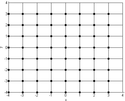
Definition 3.1. An N ×N image region is a square whose center is at the origin of
the Cartesian plane, and which is subdivided into N2 equal pixels by an N2-element
grid.
Definition 3.2. An imagef is a function of two variables whose value in the interior
region of any pixel of an N2-element grid is uniform.
Figure 3.1: A 8×8 image region.
As shown in Figure 3.1, the center pixel (0,0) of the image region has its lower-left
corner located at the origin of the Cartesian plane. For our purposes, we consider
gray-scale images f where f(i, j) represents the pixel intensity at the integral point
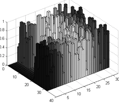
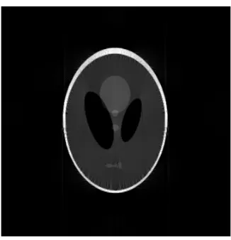
(i, j). The gray-scale Shepp-Logan phantom head, such as in Figure 3.2, can be
represented on such an image region. To see what this would look like, refer to
Figure 3.3, which shows a 32×32 image being represented on a 32×32 image region.
The height of each bar represents the intensity of the pixel at the lower-left corner of
the square it is defined on.
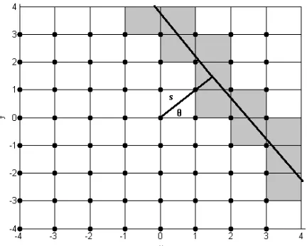
Returning our attention to the problem of acquiring the projection dataRf (θ, s),
we will denote byP(θ,s) the set of pixels intersected by the line with distance s from
Figure 3.2: A 256×256 Shepp-Logan phantom head.
Figure 3.3: A representation of a 32×32 image on an image region.
then we defineP(θ,s) as below.
P(θ,s) ={(x, y)∈Z2 |x, y ∈S, pixel at (x,y) is intersected} (3.3)
Figure 3.4 shows an example of a set of pixels being intersected by one possible line.
Using this definition, we can define the line integral which will be used in our discrete
Radon transform algorithms in the following manner.
Definition 3.3. Let P(θ, s) be known within an image region of size N ×N. Then,
Figure 3.4: The pixels intersected by the line parameterized by (θ, s).
s from the origin and an angle θ from the positive x-axis is approximated by the
weighted sumLˆf(θ, s)over the pixels in the interior of the image region. Specifically,
ˆ
Lf(θ, s) is defined as
ˆ
Lf(θ, s) :=
X
i∈S
X
j∈S
w(θ,s)(i, j)f(i, j), (3.4)
where
w(θ,s)(i, j) :=
l, if (i, j)∈P(θ,s)
0, if (i, j)∈/ P(θ,s),
(3.5)
and l is defined as the length of the intersection.
In this manner, we see that the problem of reconstructing an image f from its
projection data is a problem of solving a system of linear equations. Assuming we
acquire the projections of f along a set of lines parameterized by a set of angles
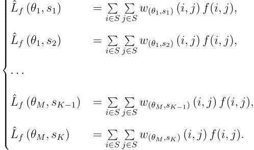
projection data as a system of linear equations, ˆ
Lf(θ1, s1) = P
i∈S
P
j∈S
w(θ1,s1)(i, j)f(i, j),
ˆ
Lf(θ1, s2) = P
i∈S
P
j∈S
w(θ1,s2)(i, j)f(i, j),
· · ·
ˆ
Lf(θM, sK−1) = P
i∈S
P
j∈S
w(θM,sK−1)(i, j)f(i, j),
ˆ
Lf(θM, sK) = P i∈S
P
j∈S
w(θM,sK)(i, j)f(i, j).
Thus, we can equivalently express the acquisition of projection data in terms of
matrices. Letting L denote the left-hand side of the above equations, W denote the
M K ×N2 matrix containing the weights, and F denote the N2 ×1 image vector
containing the pixel intensity information for f, the above system of equations can
be rewritten as the matrix equation
L=WF. (3.6)
Figure 3.5: The length, l=√∆x2+ ∆y2, of an intersection.
The basic structure of an algorithm that can be used in order to compute the
set of projection data L is divided into several steps, detailed below. Note that
computation time can be cut by first determining the left, right, top, and bottom
left, right, top, and bottom exits. Computing these locations as a first step makes it so
that we can restrict our search in terms of determining the weights of the intersections
by eliminating pixels which are most definitely not intersected. Though algorithms
A.1 and A.2 differ in a few respects, they both make use of the following general
outline.
• Step 1: For θ∈Θ and s∈Λ, compute P(θ,s).
• Step 2: Determine left, right, top, and bottom exits for the line parameterized
by (θ, s).
• Step 3: Scan through pixels between left, right, top, and bottom exits to
deter-mine the lengths of intersection.
• Step 4: Multiply the lengths by their respective pixel values (determined by f)
and add this to a running sum representing ˆLf(θ, s).
• Step 5: Repeat the process for eachθ ∈Θ ands ∈Λ.
The algorithms we present in A.1 and A.2 serve as ways of computing the discrete
line integral of an image f along a line parameterized by (θ, s). Both of these
algo-rithms make use of the fact that for θ ∈ (0, π/2), the line will be decreasing as we
move from the left exit to the right exit and therefore, the top exit will come before
the bottom exit. Alternatively, for θ ∈ (π/2, π), the bottom exit will occur before
the top exit as we move from the left exit to the right exit. In this manner, the way
we search through the potentially intersected pixels is characterized by the range in
which θ occurs.
If θ = 0 or θ =π, then the line is vertical and we merely use the distance s from
the origin to find the “column" in which the line occurs. Every pixel in this column
is intersected by the line and the length of the intersection is 1. Similarly, if θ=π/2,
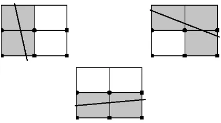
Figure 3.6: Some of the various ways a line can intersect a pixel.
the line occurs. Every pixel in this row is intersected by the line and the length of
the intersection is also 1. We should note that as θ gets close to 0 orπ, the slope of
the line parameterized by θ goes towards infinity. This causes some blurring when
reconstructing f using the projection data, as we see in Figure 3.8.
Figure 3.7: Reconstruction of Shepp-Logan Phantom head using data from Algorithm A.1.
Beyond this, the algorithms given in A.1 and A.2 essentially differ in the way we
characterized the weights assigned to the lengths of the intersection between a line
parameterized by (θ, s) and P(θ,s). Algorithm A.1 explicitly calculates the lengths of
the intersections for every point in P(θ,s), while Algorithm A.2 makes use of linear
interpolation. Algorithm A.2 first finds all of thexorycoordinates of the intersection
Figure 3.8: Reconstruction of Shepp-Logan Phantom head using data from Algorithm A.2.
determine the y or x coordinates, respectively. From here, the algorithm uses these
coordinates to “split" the pixel, and subsequently places the pixel values (weighted
by the manner in which they were split) into bins of size 1.
Due to the fact that Algorithm A.1 explicitly calculates the lengths of the
intersec-tions, it naturally has to take into account the various ways pixels can be intersected
(see Figure 3.6). Hence, further conditionals are placed within the pixel search, which
causes computation time to increase. However, it should be noted that while
Algo-rithm A.2 is faster than AlgoAlgo-rithm A.1, it is not as accurate due to the way we
calculate the weights of the intersections. It was found that this difference in
accu-racy was mostly evident when Λ = {sk}Kk=1 was chosen in a manner such that the
values sk were not uniformly distributed fork = 1,2, . . . K.
On a final note, we would like to remind the reader that Algorithms A.1 and
A.2 merely only serve the function of calculating the discrete line integral of f for a
specific line. Algorithm A.3 ties this together by utilizing these algorithms in order to
calculate the projection data of a given imageffor a given angle set Θ and distance set
Λ. Assuming|Θ|=M and |Λ|=K, the output of Algorithm A.3 is aK×M matrix,
projection matrix L described in (3.6). From this point, an inverse radon transform
algorithm can be applied to reconstruct images, such as in Figures 3.7 and 3.8 where
Chapter 4
Sub-Exponential Localization Properties of
Needlets
In the next chapter, we will introduce a new inversion formula for the Radon
trans-form based on kernels and frames which we refer to as needlets. The term needlet
comes from the fact that kernels of the form (5.1) exhibit subexponential localization
properties (i.e. they are extremely well-localized). In this chapter, we develop and
illustrate these properties in rigorous detail. The discussion begins by introducing
the class of functions known as the Schwarz class.
Definition 4.1. Let f ∈ Rn, n ≥ 1. Then, f is said to be rapidly decreasing if for every integer N ≥0, there exists a constant CN such that
|f(x)| ≤ CN
(1 +|x|)N
for all x∈Rn. We denote the space of rapidly decreasing functions by D(
Rn).
Definition 4.2. The Schwartz class S is defined to be
S(Rn) :={f ∈C∞(Rn)|f, f0, f00, . . .∈ D(Rn)}. (4.1)
Recalling the form of the kernels of interest,
Ln(x, y) =
∞ X
j=1
ˆ
a
j
n
Uj(x)Uj(y),
it will take a series of theorems, corollaries, and lemmas to prove the following result,
Theorem 4.3. Let 0≤θ, φ ≤π, and suppose ˆa∈ S(R) is an even function. Then, for any σ >0, there exists a constant cσ >0 such that
|Ln(cosθ,cosφ)| ≤
cσn
(sinθ+n−1) (sinφ+n−1) (1 +n|θ−φ|)σ.
It follows as an immediate corollary from our primary claim that for x, y ∈R,
|Ln(x, y)| ≤
cσn
√
1−x2+n−1 √1−y2+n−1(1 +nρ(x, y))σ, (4.2)
where ρ(x, y) =|arccosx−arccosy|.
Theorem 4.4. Let P be an arbitrary constant. For appropriate functions g,
X
j∈Z
g(P j) = 1
P
X
j∈Z ˆ
g(j).
The equation given by Theorem 4.4 is known as the Poisson summation formula
and is necessary to prove the following lemma.
Lemma 4.5. Consider the trigonometric polynomial given by
Fn(θ) =
X
j∈Z ˆ
a
j
n
eijθ, (4.3)
where ˆa ∈ C∞(R) and supp ˆa ∈ [−2,2]. Then, for any σ > 0, there exists cσ > 0 such that
|Fn(θ)| ≤
cσn
(1 +n|θ|)σ, θ ∈[−π, π]. (4.4)
Proof. Letf be defined in terms of its Fourier transform
ˆ
f(ξ) := ˆa ξ n
!
eiξt.
Then, it follows that
f(y) = 1 2π
Z
R ˆ
f(ξ)eiξydξ
= 1 2π Z R ˆ a ξ n !
eiξteiξydξ
= 1 2π Z R ˆ a ξ n !
Letting u=ξ/n, it follows that dξ =ndu and the former yields
f(y) = na(n(t+y)). (4.5)
Now,
|Fn(θ)|=
1 2 X
j∈Z ˆ a j n eijθ = 1 2 X
j∈Z ˆ
f(j) .
From Theorem 4.4, we obtain
|Fn(θ)|=π
X
j∈Z
f(2πj).
From here, (4.5) yields
|Fn(θ)|=πn
X
j∈Z
a(n(θ+ 2πj)).
Now, ˆa ∈ C∞(R) is of compact support and so it follows that ˆa ∈ S(R). To see
this, simply note that any derivative of ˆais supported on supp (ˆa) and therefore also
has compact support. Hence, any derivative of ˆais thereby bounded by the Extreme
Value Theorem. Thus, it follows that for any σ >0, there exists cσ >0 such that
X
j∈Z ˆ
a(n(θ+ 2πj))≤X
j∈Z
cσ
(1 +n|θ+ 2πj|)σ
= cσ
(1 +nθ)σ + X
j6=0
cσ
(1 +n|θ+ 2πj|)σ.
Recall that −π ≤θ≤π. Then, the foregoing becomes
X
j∈Z ˆ
a(n(θ+ 2πj))≤ cσ
(1 +n|θ|))σ + X
j6=0
cσ
(1 +n|πj|)σ.
From here, simple quantitative arguments yield our desired result:
X
j∈Z ˆ
a(n(θ+ 2πj))≤ cσ
(1 +n|θ|)σ + ∞ X
j=1
cσ
Lemma 4.6. Suppose 0 ≤ θ, φ ≤ π. Then, for any σ > 0 there exists a constant
cσ >0 such that
|Fn(θ)| ≤
cσn
(1 +n|θ−φ|)σ. (4.6)
Proof. Letσ > 0 be given. We consider the following two cases.
• Case 1: Suppose θ+φ ≤π. Then,θ+φ ≥ |θ−φ| and therefore, from (4.4) it
follows that
|Fn(θ+φ)| ≤
cσn
(1 +n|θ+φ|)σ
≤ cσn
(1 +n|θ−φ|)σ.
• Case 2: Suppose θ+φ > π. Then, 0<2π−θ−φ≤π. Lettingα=π−θ and
β =φ−θ, it follows that 2π−θ−φ=α+β. Furthermore, 0≤α, β ≤π and
α+β ≥ |α−β| =|θ−φ|. Coupling this with (4.4) and the fact that Fn is an
even function yields
|Fn(θ+φ)|=|Fn(2π−θ−φ)|
≤ cσn
(1 +n|2π−θ−φ|)σ
≤ cσn
(1 +n|θ−φ|)σ.
From above, we obtain the following corollary.
Corollary 4.7. Let 0< θ, φ < π. Then, for anyσ >0 there exists a constant cσ >0
such that
|Ln(cosθ,cosφ)| ≤
cσn
Proof. From (5.1), we observe that for 0< θ, φ < π,
Ln(cosθ,cosφ) =
∞ X
j=1
ˆ
a
j
n
sin(jθ) sin(jφ)
sinθsinφ .
By adding/subtracting the term ˆa(0)/2 to the aforementioned expression and
subse-quently applying a product-to-sum trigonometric identity, we obtain that
Ln(cosθ,cosφ) =
1 2 sinθsinφ
∞ X
j=1
ˆ
a
j
n
[cos (j(θ−φ))−cos (j(θ+φ))].
Then, by (4.3), the former becomes
Ln(cosθ,cosφ) =
1
2 sinθsinφ(Fn(θ−φ)−Fn(θ+φ)), (4.8)
and therefore, from (4.6), it follows that
|Ln(cosθ,cosφ)| ≤
cσn
sinθsinφ(1 +n|θ−φ|)σ.
Lemma 4.8. Let 0≤ θ, φ ≤π. Then, for any σ >0 there exists a constant cσ >0
such that
|Ln(cosθ,cosφ)| ≤
cσn3
(1 +n|θ−φ|)σ. (4.9)
Proof. An important formality we must address is that throughout the proof of this
lemma, the constant cσ may change and, hence, may represent a different constant
from instance to instance. However,cσ will always be dependentonly onσ. The
deci-sion to leave its notation unchanged is a matter of choice based on visual organization
and aesthetic, and leaves the validity of the proof intact.
Let Gn be the function defined by
Gn(x) :=
∞ X
j=1
ˆ
a
j
n
whereUj is ajth Chebyshev Polynomial of the Second Kind as defined in (2.3). Now,
from (4.3), it follows that
Fn(x) =
ˆ a(0) 2 + ∞ X j=1 ˆ a j n
Tj(x),
where Tj is jth Chebyshev Polynomial of the First Kind as defined in (2.2). Then,
Fn(cosθ) =
ˆ a(0) 2 + ∞ X j=1 ˆ a j n cosjθ.
Taking the derivative with respect to θ yields
d
dθ [Fn(cosθ)] = −
∞ X j=1 ˆ a j n
jsinjθ,
and so it follows that
Fn0(x) = ∞ X j=0 ˆ a j n
jUj(x) = Gn(x). (4.11)
We now recall the Markov inequality which states that for any Pm ∈Πm, m ≥0
and a, b∈R,
kPm0 kL∞[a,b]≤
2n2
b−akPmkL∞[a,b].
Since Fn ∈ Π2n, it follows from (4.11) and the above Markov inequality that for
t∈[−1,1],
kGnkL∞[−1,t]=kF
0
nkL∞[−1,t]
≤ 2n
2
t+ 1kFnkL∞[−1,t].
From (4.6), the foregoing becomes
kGnkL∞[−1,t]≤
2n2 t+ 1
cσn
1 +n√1− •σ
L∞[−1,t] .
Note that if t∈[0,1], then the function
attains its maximum att on the interval [0, t]. This follows from the fact that h is a
monotonically increasing function on [−1,1]. This readily leads us to
kGnkL∞[−1,t]≤
2n2
t+ 1
cσn
1 +n√1− •σ
L∞[−1,t]
≤ 2n
2
t+ 1
cσn
1 +n√1−tσ
= cσn
3
(t+ 1)1 +n√1−tσ.
By similar reasoning, for allt∈[−1,0], the aforementioned functionhis bounded
above on the interval [−1, t] by the case whent= 0 and so it follows that
kGnkL∞[−1,t]≤
cσn3
(1 +n)σ
≤ cσn
3
1 +n√1−tσ,
where the last inequality results from scaling of the constant cσ. Hence, it follows
that for all t∈[−1,1],
kGnkL∞[−1,t]≤
cσn3
(t+ 1)1 +n√1−tσ. (4.12)
We now refer to a product formula for Gegenbauer polynomials, of which
Cheby-shev polynomials are a specific type, as presented in [5]. Specifically, it follows from
this product formula that for some constant c,
Uj(cosθ)Uj(cosφ) Uj(1)
=c
Z 1
−1
Uj(cosθcosφ+usinθsinφ)du,
and so therefore,
Ln(cosθ,cosφ) =
∞ X j=1 ˆ a j n
Uj(cosθ)Uj(cosφ)
=c Z 1 −1 ∞ X j=1 ˆ a j n
Uj(1)Uj(cosθcosπ+usinθsinφ)du.
Now, Uj(1) = limθ→0(sinjθ/sinθ) = j and so the former becomes
Ln(cosθ,cosφ) =c
Z 1 −1 ∞ X j=1 ˆ a j n
Letting t(u, θ, φ) = cosθcosφ+usinθsinφ and by using (4.12), we obtain that
|Ln(cosθ,cosφ)| ≤
Z 1
−1
cσn3
1 +nq1−t(u, θ, φ)σ
du. (4.13)
Note that for 0≤θ, φ≤π, it follows that sinθsinφ≥0 and so
1−t(u, θ, φ) = 1−cosθcosφ−usinθsinφ
≥1−cosθcosφ−sinθsinφ
= 1−cos(θ−φ)
= 2 sin2(θ−φ).
Furthermore, 2 sin2(θ−φ) is equivalent to (θ −φ)2 (up to some scalar value) when
0≤θ, φ≤π. Combining this fact with the above inequality, (4.13) becomes
|Ln(cosθ,cosφ)| ≤
cσn3
(1 +n|θ−φ|)σ.
Lemma 4.9. Let θ, φ≥0. Then
θ+n−1 φ+n−1≤3
θφ+ 1
n2
(1 +n|θ−φ|), n ≥1. (4.14)
Proof. Without relevant loss of generality, suppose φ ≥ θ. Then, for some λ ≥ 1,
φ=λθ. Note that proving (4.14) is equivalent to proving the inequality
θφ+ 1
n2 +
θ+φ
n ≤3θφ+
3
n2 + 3θφn|θ−φ|+
3|θ−φ|
n ,
and so it suffices to prove that
θ+φ
n ≤2θφ+
2
n2 + 3θφn|θ−φ|+
3|θ−φ|
n . (4.15)
• Case 1: Suppose λ ≥ 3. Then, (θ + φ)n−1 ≤ (3|θ−φ|)n−1 if and only if
λ+ 1≤3 (λ−1). Yet this is true if and only if 4≤ 2λ, which is equivalent to
the condition thatλ≥2.
• Case 2: Suppose that 1≤λ <3. Then,
θ+φ
n ≤2
θφ+ 1
n2
if and only if
(λ+ 1)θ
n ≤2
λθ2+ 1
n2
.
This inequality holds so long as
4θ n ≤2
θ2+ 1
n2
,
which is equivalent to the condition thatθ2−2θn−1+n−2 ≥ 0. Factoring this
expression tells us that (θ−n−1)2 ≥0, which is clearly true. Therefore,
θ+φ
n ≤2
θφ+ 1
n2
,
implying the validity of (4.15).
We are finally ready to prove the primary localization result of this chapter.
Proof of Theorem 4.3. The proof is divided into three cases.
• Case 1: Suppose 0≤ θ ≤2π/3 and 0≤φ ≤ π/2. Now, sinθsinφ ∼ θφ (up to
some scalar value) and so from (4.7), it follows that
|Ln(cosθ,cosφ)| ≤
2cσn
2θφ(1 +n|θ−φ|)σ. (4.16)
Furthermore, from (4.9), we achieve
|Ln(cosθ,cosφ)| ≤
2cσn
2n−2(1 +n|θ−φ|)σ. (4.17)
– Case 1a: Supposeθφ≤n−2. Then,θφ+n−2 ≤2n−2 and so it follows from
(4.17) that
|Ln(cosθ,cosφ)| ≤
2cσn
– Case 1b: Suppose that θφ > n−2. then, θφ+n−2 ≤2θφ and so by (4.16)
it follows that
|Ln(cosθ,cosφ)| ≤
2cσn
(θφ+n−2) (1 +n|θ−φ|)σ.
Combining Cases 1a and 1b, we obtain the inequality
|Ln(cosθ,cosφ)| ≤
cσn
(θφ+n−2) (1 +n|θ−φ|)σ,
and so therefore,
|Ln(cosθ,cosφ)| ≤
cσn
(θφ+n−2) (1 +n|θ−φ|)σ
≤ 3cσn
3 (θφ+n−2) (1 +n|θ−φ|) (1 +n|θ−φ|)σ−1.
Lettingσ0 =σ−1 and using the result given by (4.14), we achieve the following
result that
|Ln(cosθ,cosφ)| ≤
cσ0n
(θ+n−1) (φ+n−1) (1 +n|θ−φ|)σ0.
Since sinθ ∼θ,sinφ∼φ, andσ is arbitrary, the foregoing yields
|Ln(cosθ,cosφ)| ≤
cσn
(sinθ+n−1) (sinφ+n−1) (1 +n|θ−φ|)σ.
• Case 2: Suppose that π/3 ≤ θ ≤ π and π/2 ≤ φ ≤ π. Then, 0 ≤ π −
θ ≤ 2π/3 and 0 ≤ π − φ ≤ π/2. Note that cos (π−θ) = −cosθ and
cos (π−φ) = −cosφ. Since Ln is an even function in two variables it follows
that Ln(cos (π−θ),cos (π−φ)) = Ln(cosθ,cosφ). Hence, the result follows
from Case 1.
• Case 3: Suppose that either 0 ≤ φ ≤ π/3 and π/2 ≤ θ ≤ π or 2π/3 ≤ θ ≤ π
and 0≤φ≤π/2. Then, we have |θ−φ| ≥π/6. Hence, by (4.9) and scaling of
the constant cσ,
|Ln(cosθ,cosφ)| ≤
4cσn3
Yet, (sinθ+ 1/n) (sinφ+ 1/n)≤4 and so
|Ln(cosθ,cosφ)| ≤
cσn
(sinθ+n−1) (sinφ+n−1) (1 +n|θ−φ|)σ.
From Cases 1, 2, and 3, the complete result follows.
As mentioned in the beginning of this chapter, the above proof yields (4.2) as an
immediate corollary. That is, for any σ >0 there exists a constant cσ >0 such that
|Ln(x, y)| ≤
cσn
√
1−x2+n−1 √1−y2+n−1(1 +nρ(x, y))σ,