CHANNEL ESTIMATION USING EXTENDED VERSION OF KALMAN FILTER FOR 2 X 2 MIMO SYSTEMS

CHANNEL ESTIMATION USING EXTENDED VERSION OF

KALMAN FILTER FOR 2 X 2 MIMO SYSTEMS

*Anirudh Mudaliar

**Rakesh Mandal

***Sunil Kumar Vishwakarma

ABSTRACT

This paper proposes Robust Kalman Filter (RKF) for channel estimation in wireless network.

Today various Multi-user Detection(MUD) are used for channel estimation. This paper compares

the performance of RKF with popular MUD’s like SIC and PIC and propose RKF to is

beneficial. The paper briefly discusses the advantages of Multiple Input and Multiple Output

(MIMO) systems with Orthogonal Frequency Division Multiple (OFDM) technique and tells

why they are so popularly used. Then performance of SIC and PIC are discussed briefly. The

need for Kalman Filter (KF) is then explained along with algorithm and performance of RKF and

finally the performance comparison of all the above mentioned techniques is provided to show

that RKF is beneficial for channel estimation in today’s scenario.

Keywords- Discrete time system, Time-delay, KF, RKF, Kalman gain, SIC , PI

* Asstt. Professor, SSTC, Bhilai

**Asstt. Professor, SSTC, Bhilai

1. INTRODUCTION

The channel estimation is the process of characterizing the effect of channel over the transmitted

signal. The channel provides Multipath fading due to which ISI, ICI and Selective Frequency

Fading occurs in general. For efficient working of wireless systems various techniques are

available like OFDM ,MIMO, RAKE receiver etc. Researchers have shown that of the available

techniques MIMO assisted OFDM is more beneficial.

Multiple Input and Multiple Output (MIMO) Systems:

As indicated by the terminology, a MIMO system employs multiple transmitter and receiver

antennas for delivering parallel data streams, Since the information is transmitted through

different paths, a MIMO system is capable of exploiting both transmitter and receiver diversity,

hence maintaining reliable communications.

Briefly, compared to single-input single-output (SISO) systems, the two most significant

advantages of MIMO systems are as follows.

A significant increase of both the system’s capacity and spectral efficiency. The capacity

of a wireless link increases linearly with the minimum of the number of transmitter or the

receiver antennas. The data rate can be increased by spatial multiplexing without

consuming more frequency resources and without increasing the total transmit power.

Dramatic reduction of the effects of fading due to the increased diversity. This is

particularly beneficial, when the different channels fade independently.

Orthogonal Frequency Division Multiplexing (OFDM) Technique:

OFDM is a multi carrier system. There are two main advantages of OFDM:

1. Reduces ISI and ICI

2. Selective Frequency Fading

The quality of wireless link can be described by three parameters, namely transmission rate,

transmission range and the transmission reliability. With the advent of MIMO assisted OFDM

systems, all the three parameters may be simultaneously improved. Furthermore, recent research

suggests that the implementation of MIMO-aided OFDM is more efficient than other techniques.

CHANNEL ESTIMATION USING SIC:

In SIC-aided SDMA-OFDM MUDs the following operations are carried out for all subcarriers.

a) Arrange the detection order of users upon invoking an estimate of the total signal power

received by each individual user on the different antenna elements and detect the highest-power

user’s signal using the above-mentioned MMSE detector, since it is the least contaminated by

multiuser interference (MUI).

b) Then re-generate the modulated signal of this user from his/her detected date and subtract it

from the composite multiuser signal.

c) Detect the next user according to the above procedure by means of MMSE combining, until

the lowest-power signal is also detected, which has by now been “decontaminated” from the

MUI.

d) Since the lowest-power user’s signal is detected last, a high diversity gain is achieved by the

MMSE combiner, which, hence, mitigates not only the effects of MUI but also that of channel,

fades.

e) It has to be note, however that the SIC MUD is potentially prone to user-power classification

errors as well as to inter-user error propagation, since in case of detection errors the wrong

re-modulated signal is deducted from the composite multiuser signal. Hence, this technique is

beneficial in near-far scenarios encountered in the absence of accurate power control.

CHANNEL ESTIMATION USING PIC:

By contrast, PIC dispenses with user-power classification all together, hence avoiding the

above-mentioned potential mis-classification problem. It has benefits in more accurately power

controlled scenarios. Its philosophy is briefly summarized as follows.

• On the basis of the composite received multiuser signal vector x generate an estimate of all user

signals y(t) emplying the above-mentioned MMSE detection;

b) If channel encoding was used, decode, slice and channel encode again as well as re-modulate

the each user’s signal on an OFDM subcarrier basis.

c) Second detection iteration for all subcarriers:

• reconstruct the signal vectors x (l) of all users;

• generate an estimate y(k) of all user signals by subtracting the signal vectors x(l) , l k of all

the other users followed by the above mentioned MMSE combining.

d) Channel decode and slice the extracted user signals in order to generate b(l).

e) Despite the absence of power-classification errors the PIC technique is also sensitive to

inter-user error propagation.

Channel Estimation Using Kalman Filter:

The Kalman filter is a mathematical power tool that is playing an increasingly important role in

computer graphics as we include sensing of the real world in our systems. The good news is you

don’t have to be a mathematical genius to understand and effectively use Kalman filters. This

tutorial is designed to provide developers of graphical systems with a basic understanding of this

important mathematical tool.

Finite time can be expressed as the following five steps:

1.) State Estimate Extrapolation(propagation)

2.) Covariance Estimate Extrapolation(propagation)

3.) Filter Estimate Update

4.) State Estimate Update

5.) Covariance Estimate “Update”

We use a KF to estimate the state

n k

x ∈ ℜ

of a discrete time controlled system. The system is

described by a linear stochastic difference equation.

1

k k k

x+ = Ax +Bw _(2.1)

k k k

y =Cx +v

where,

n k

x ∈ ℜ

is the system state,

m k

y ∈ ℜ

is the measured output,

q k

w ∈ ℜ

is the process

noise,

p k

v ∈ ℜ

is the measurement noise. In the following vk _and wk_{will be the process of}

finding the “best estimate” from noisy data amounts to “filtering out” the noise.

However a Kalman filter also doesn’t just clean up the data measurements, but also projects

these measurements onto the state estimate.

2. KALMAN FILTERING FOR LINEAR DISCRETE TIME SYSTEM

Kalman Filter (KF) is a numerical method used to track a time-varying signal in the presence of

noise. It is the problem of estimating the instantaneous state of a linear system from a

measurement of outputs that are linear combinations of the states but corrupted with Gaussian

white noise. The resulting estimator is statically optimal with respect to a quadratic function of

estimation error. From the mathematical point view, the KF is a set of equations that provides an

efficient recursive computational solution of the linear estimation problem. The filter is very

powerful in several aspects. The KF is an extremely effective and versatile procedure for

combining noisy sensor outputs to estimate the state of the system with uncertain dynamics.

When applied to a physical system, the observer or filter will be under the influence of two noise

sources: (i) Process noise, (ii) Measurement noise. The estimate of the state is specified by its

conditional probability density function. The purpose of a filter is to compute the state estimate,

while an optimal filter minimizes the spread of the estimation error probability density. A

recursive optimal filter propagates the conditional probability density function from one

sampling instant to the next, keeping in view the system dynamics and inputs, and it incorporates

measurements and measurement errors static in the estimate.

Regarded as zero mean, uncorrelated white noise sequence with covariance Rk_andQk_.

vk =N

(

)

The matrix A∈ ℜn n× in the difference Equation (2.1) is the dynamics matrix which relates the sate at time step kto the sate at time stepk+1. The matrix B∈ ℜn×1 called noise matrix. The matrix C∈ ℜm m× in the measurement Equation (2.2) relates the state measurementyk_.

The KF algorithm can be seen as a form of feedback estimation. The set of the KF equation can

be separated in two groups:

1. Time update equations

2. Measurement update equation

The time update equations project the current state and the error covariance estimates forward in

the time to obtain a priori estimates for the next time step. The measurement update equations

handle the feedback. In other words, it incorporates a new measurement into the a priori estimate

to obtain a corrected a posterior estimate. Therefore the time update equations are predicator

equations, and the measurement update equations are corrector equations. That is, the KF is a

predictor-corrector algorithm to provide a recursive solution to the discrete time linear system, as

shown in Fig. 2.1.

FIGURE 2.1: Discrete Kalman Filter Cycle

The time and measurement update equations are presented below:

The time and measurement update equations are presented below:

The time updates equations:

xˆk 1 Axˆk Buk

−

+ = + (2.5)

1

T

k k k k

P−+ = AP A +Q (2.6)

The measurements update equations:

(

)

1

T Y

f k k k k k k

K =P C− C P C− +R − (2.7)

(

)

ˆ_k ˆ_{k f k k}ˆ_k

x =x +K y −C x− (2.8)

P_k =

(

)

The time-update equation projects the state estimate and covariance from time stepkto stepk+1. To compute the Kalman Gain (KG) K_fis the first job in the measurement update equations. Theny_k is obtained by actual measurement of the system. Incorporating the actual measurement and the estimated one in equation (2.7), we generate a posterior estimate. The last step is to

compute a posterior error covariance. This is the recursive operation of the KF. A complete

picture of the operation of the KF is illustrated in Fig. 2.2, after each time and measurement

update pair, the recursive algorithm is repeated with the previous a posterior estimates to predict

the new a priori estimates. This recursive nature is the biggest advantage of the KF. This makes

the practical implementation of the KF much easier and feasible then the implementation of the

Wiener filter, because the Weiner filter obtains its estimates by using all of the precedent data

directly. In contrast, the KF only uses the immediately previous data to predict the current states

[9].

Robust Kalman Filter (RKF) :

The RKF is a robust version of the KF but with necessary modification to account for the

parameter uncertainty. The RKF usually yields a suboptimal solution with respect to the nominal

system but it guarantees an upper bound to the filtering error covariance in spite of large

parameter uncertainties. The standard KF approach does not address the issue of robustness

against large parameter uncertainty in the linear process model. The performance of a KF may be

significantly degraded if the system having uncertainty. To avoid this problem RKF is used, the

to an uncertain dynamical system rather than a known linear system. In this chapter, we consider

the problem of Robust Kalman Filtering for discrete-time systems with norm-bounded parameter

uncertainty in both the state and output matrices [2].The Algorithm for RKF is as follows:

System Equation

Measurement Equation

These uncertainties are assumed to be the following structure

Robust Kalman Filter Equation

Kalman gain

Covariance of estimation error

Covariance of process noise

Covariance of measurement noise

Covariance of true state

(

)

1

k k k k k k

x + = A + ∆A x +B w

(

)

y= C+ ∆C x +v

& k k A C ∆ ∆ 1 2 k k k A H F E C H ∆ = ∆

(

)

(

)

ˆ_{k ek} ˆ_{k f k ek} ˆ_k

x ₊ = A+ ∆A x +K y − C+ ∆C x

(

)

1 2

1

T T T

f k k k

k

K AQ C _ε H H Rε CQ C −

= + +

(

)

T T

ek k k k k

A ε AS E I ε ES E − E

∆ = −

(

)

T T

k k k k

C ε AC E I ε ES E − E

∆ = −

(

)

f ek

A = A+ ∆A

1

1 1 1 1 1

T T T T T T

k k k k k

k

P AP A H H BWB APE I EPE EP A

ε ε

−

+ = + + + −

1 1 T

k k k

Q − S − ε E E

= −

1

2 2

T

k k

R_ε V ε− H H

4. RESULTS & SIMULATIONS

4.1 Simulation Result of Kalman Filter

Consider the following discrete time system,

[

]

1

0

0.5

6

1

1

1

100 10

k k k

k k k

x

x

w

y

x

v

+

−

−

=

+

= −

+

Note that the above system is of the form of system with 1 0 , 1, 1

0 1

P=S = W = V =

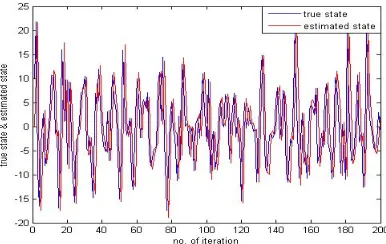
FIGURE 4.1: No. of Iteration vs. True State and Estimated State

FIGURE 4.2: No. of Iteration vs. Eigen Value of Covariance Matrix.

(

)

1 1 1

1 1 2 1 2 1 1 1

T T T

k k

T T T

k k k

k

T T

k

k

S A Q A H H B W B

A Q C H H R C Q C

A Q C H H

4.2COMPARISON OF MUD’S

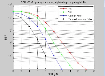
Figure 4.3 : BER vs SNR for 2x2 MIMO System

5. CONCLUSION

The simulation result of Kalman Filter and State Estimation using Kalman Filter in problem.

Fig.4.3 shows the estimated states by KF and true state of a system which is considered. And we

observe from the figure that estimated state is nearly equal to true state with some error. The

estimation error increases in the system having uncertainty.

Finally after comparing the simulation results of SIC, PIC, KF and RKF, we conclude that

performance of RKF is satisfactory as compared to others.

6. REFERENCES

[1] Munmun Dutta, Balram Timande and Rakesh Mandal, “ROBUST KALMAN FILTERING

FOR LINEAR DISCRETE TIME UNCERTAIN SYSTEMS”, IJAET , Vol. 4, Issue 2, pp.

276-283(2012).

[2] Mital A Gandhi, and Lamine Mili, “Roust Kalman Filter based on a Generalized Maximum-

Likegood-Type Estimator”, IEEE Transaction on Signal Processing, Volume 58,

[3] Rodrigo Fontes Souto and Joao Yoshiyuki Ishihara, “Robust Kalman Filter for Discrete-Time

Systems With Correlated Noise”, Ajaccio, France, 2008.

[4] X.Lu, H.Zhang and W.Wang, “Kalman Filtering for Multiple Time Delay System”,

Automatica, Volume 41, pp- 1455-1461 (2005).

[6] Z.Wang, J.Lam and X.Liu, “Robust Kalman filtering for Discrete-Timr Markovian Jump

Delay Sustem”, IEEE Signal Processing Letters, Volume 11, pp- 659-662 (2004).

[7] Ming Jian and Lajos Hanzo, “Multi-user MIMO-OFDM for next Generation Wireless

Systems”, Proceedings of the IEEE | Vol. 95, No. 7, July 2007.

[8] M. Huang, X. Chen, L. Xiao, S. Zhou and J. Wang, “Kalman Filter Based OFDM Systems in