Deterministic & Un-deterministic Network Flow Problems

(1)

Deterministic & Un-deterministic Network Flow Problems

Radhe Shyam Soni1, Dr. S.P. Varma2 1

Assistant Professor, Department of IT, L.N.Mishra College of Business Management Muzaffarpur,

2

Ex-Associate Professor, P.G. Department of Mathematics, B.R.A. Bihar University, Muzaffarpur

Abstract:

In day to day life one often feels problem in planning a tour which is less time and distance consuming. Sometimes a tour is planned easily under known situations but sometimes a tour is to be planned under unknown situations. In this condition uncertainly theory comes into play. We propose to discuss such problems in this paper.

Keywords: Graph Theory, Network Flow Problems, Uncertain Network, Uncertainty Theory, Un-deterministic Network Flow Problem, .

[1] Introduction

In practical situations, un-deterministic factors are frequently encountered. This paper represents two types of approaches for a person who wants to plan a tour from one location to another location. First approach uses classical deterministic method or traditional method and the other uses uncertainty theory which is powerful tool in the field of uncertain environment.

Here networks are presented through a graph where vertices are represented by circles and edges are represented by lines. A line contains some values called weight. In another word, we can say that it is a weighted graph. For uncertain network, the weight of edges is approximately estimated by an expert. In this paper three types of optimal tour model: Expected optimal Tour, ∝ - Optimal Tour and Distribution Optimal tour have been proposed. Where expected optimal tour provides an average value of uncertain measure, ∝ - optimal tour is a predetermined confidence level provided by the expert and Distribution optimal tour is a carrier of incomplete information of uncertain variable respectively.

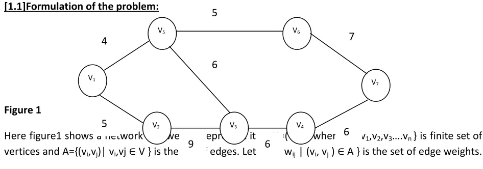
[1.1]Formulation of the problem:

Figure 1

Here figure1 shows a network and we can represent it as N=(V,A), where V={v1,v2,v3….vn } is finite set of vertices and A={(vi,vj)| vi,vj ∈ V } is the set of edges. Let w = { wij | (vi, vj ) ∈ A } is the set of edge weights.

V1

V2 V5

V4 V3

V6

V7 7

6 5

4

5

9 6

(2)

Then, the network can be denoted N = (V, A, w). A route of N is a path that traverses edge of N from one location to another location. The shortest path in this situation is to be obtained.

Generally, each wij is positive integer and the shortest route weight is a function of w which is denoted as f (w). For a network N= (V,A,w), f (w) can be obtained by any traditional method. We employ the algorithm based on Dijkstra algorithm. First we show the Dijkstra algorithm that is used to find the shortest path.

[1.2] Dijkstra Algorithm

Input: A connected weighted graph

Output: L(z), the length of shortest distance from a to z

Step 1: Set L(a)=0 and for all vertices v ≠ a, L(v) = ∝

Set T = v where T = set of vertices having temporary labels.

V=vertex set of N.

Step 2: Let u be a vertex in T for which L(u) is minimum and hence the permanent label of u.

Step 3: if u=z then stop.

Step 4: For every edge e=(u,v), incident with u, if v ∈ T, change L(v) to min ( L(v), L(u) + w(e))

Step 5: change T to T-{u} and go to step 2.

We can apply this algorithm for our required solution. Consider the network represented by figure 1 in which we have to find the shortest route from v1 to v7 (destination).

Initial table for labeling

Vertex V v1 v2 v3 v4 v5 v6 v7

L(v) 0 α α α α α α

T { v1 v2 v3 v4 v5 v6 v7 }

Iteration 1: u=v1 has L(u) = 0, T becomes T – {v1}. There are two edges incident with v1 i.e v1v2 and v1v5 where v2 and v3∈ T.

L(v2)=min {old (v2), old(v1)+w(v1v2)}

=min(α, 0 + 5} =5

(3)

=min(α, 0 +4} =4

Hence minimum label is L(v5)= 4 then.

L(v) 0 5 α α 4 α α

T { v2 v3 v4 v5 v6 v7 }

Iteration 2: u=v5, the permanent label of v5 is 4. T becomes T – {v5}. There are two edges incident with v5 i.e. v5v3 and v5v6 where v3 and v6∈ T.

=min(α, 4 + 6} =10

=min(α, 4 + 5} =9

L(v) 0 5 10 α 4 9 α

T { v2 v3 v4 v6 v7 }

Iteration 3: u=v6 , the permanent label of v6 is 9. T becomes T – {v6}. There are one edge incident with v6 i.e. v6v7 where v7∈ T.

=min(α, 9 + 7} =16

L(v) 0 5 10 α 4 9 16

T { v2 v3 v4 v7 }

Since u= v7 is the only choice, resulting stop of iteration.

Thus the shortest distance between v1 to v7 is 16 and the shortest path is (v1,v5,v6,v7).

(4)

However, when there is lack of data, some uncertain factors appear. In this situation the weighted data can be obtained from the empirical estimation. Herein uncertainty theory comes into play.

[2.1] Now we introduce some basic concepts of uncertainty theory and its properties:

Let Γ be a nonempty set, L is a σ-algebra over Γ. Each element Λ ∈L is called an event. M {Λ} is a function from L to [0, 1]. In order to ensure that the number M {Λ} has certain mathematical properties, Liu (2007, 2010c) presented the following four axioms: normality, duality, subadditivity, and product axioms. If the first three axioms are satisfied, the function M {Λ} is called an uncertain measure. The triplet (Γ, L, M) is called an uncertainty space.

Definition 1: (Liu, 2007) An uncertain variable is ameasurable function ξ from an uncertainty space (Γ, L,

M) to the set of real numbers, i.e., for any Borel set B of real numbers, the set

{ξ ∈ B } = {γ∈ Γ | ξ (γ) ∈ B} is an event.

Definition 2: (Liu, 2007) An uncertain variable ξ canbe characterized by its uncertainty distribution Φ: ℜ

→ [0, 1] , which is defined as follows

Φ(x) =M {γ∈ Γ ξ (γ) < x).

Then the inverse function Φ−1 is called the inverse uncertainty distribution of c.

Definition 3: (Liu, 2007) Let ξ be an uncertain variable.Then the expected value of ξ is defined by

E[ξ] = M ξ ≥ r dr − M ξ ≤ r dr 0

−∞

+∞

0

provided that at least one of the two integrals is finite.

Theorem 1: (Liu, 2010c)Letξ1,ξ2,L,ξn be independent uncertain variables with uncertainty distributions Φ1 , Φ2 , … , Φn, respectively. If the function f ( x1 , x2 ,…L, xn ) is strictly increasing with respect to x1 , x2 ,…, xm and strictly decreasing with respect to xm+1 , xm+2, …., xn , then

ξ=f ( x1 , x2 , …., xn )is an uncertain variable with inverse uncertainty distribution

φ-1(α)= 𝒇(𝝋_𝟏−𝟏_{𝜶 , 𝝋} 𝟐

−𝟏_{𝜶 , 𝝋} 𝟑

−𝟏_{𝜶 , … . . 𝝋} 𝒎 −𝟏_{𝜶 , 𝝋}

𝒎+𝟏 −𝟏 _{𝜶 , 𝝋}

𝒎+𝟐

−𝟏 _{𝜶 , … . . 𝝋} 𝒏 −𝟏_𝜶

Theorem 2: (Liu, 2010c) Letξandηbe independentuncertain variables with finite expected values. Then for any real numbers a and b, we have

E [aξ+bη] =aE[ξ] + bE[η].

(5)

xij : zero and one decision variable on ξij

R : a route in uncertain network N=(V,A,ξ)

F(ξ) : The shortest route weight of N=(V,A,ξ)

Ψ(x) : The uncertain distribution of f(ξ)

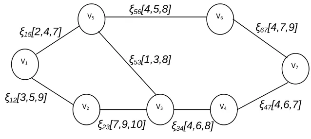
[3]Consider an uncertain network with expert’s empirical estimation information

Figure 2

Suppose that we have a network with seven vertices and eight edges. This network represents a road map of a town where vertices are a junction point to which different roads are connected. A person wants to make a plan such that the total weight (may be time, expenses or distance) on route is minimized. At first a person needs to obtain the basic data such as traffic position. So that he can plan tour. We usually cannot obtain these data exactly. Therefore we obtain these uncertain data by means of expert’s empirical estimation. Assume the network N= (V,A, ξ) as shown in figure 2 and in which ξij are zigzag uncertain variables as shown on edges.

The zigzag uncertain variable ξ=Z (a,b,c) has an uncertainty distribution

φ 𝑥 =

0 , if x ≤ a (x − a)

2 b − a , if a ≤ x ≤ b (x + c − 2b)

2 c − b , if b ≤ x ≤ c 1 , ifx ≥ c

Where a, b, c are real numbers with a ≤ b ≤ c

ξ53[1,3,8]

ξ67[4,7,9]

ξ47[4,6,7]

ξ34[4,6,8]

ξ23[7,9,10]

ξ56[4,5,8]

ξ15[2,4,7]

ξ12[3,5,9] V1

V2 V5

V4 V3

V6

(6)

The table obtains the zigzag uncertain variables that is

ξij (a,b,c) ξij (a,b,c)

ξ12 (3,5,9) ξ47 (4,6,7)

ξ15 (2,4,7) ξ53 (1,6,8)

ξ23 (7,9,10) ξ56 (4,5,8)

ξ34 (4,6,8) ξ67 (4,7,9)

Table 1

Step 1: To calculate the expected shortest route E[ξij] of ξij is as follows

ξij E[ξij] ξij E[ξij]

ξ12 5 ξ47 6

ξ15 4 ξ53 6

ξ23 9 ξ56 5

ξ34 6 ξ67 7

Table 2

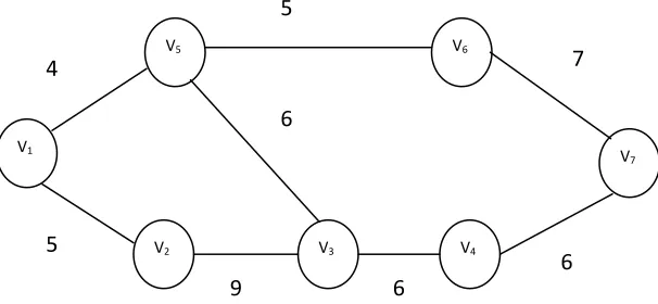
Step 2: From the table 2, we constructed a traditional weighted network as

Step 3: Employ Dijkstra algorithm then the shortest route is v1v5v6v7 so f(w) =16

According to the Theorem 3 the expected shortest route R in uncertain network N= (V, A, ξ) as

v1v5v6v7 and f (ξ) =16

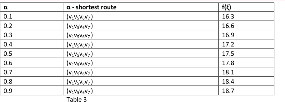
[4] ∝-Shortest Route

To calculate ∝-Shortest Route, Let ∝=0.9 from Dijkstra algorithm P=v1v5v6v7 with Φ-1 (0.9)= 4.9+5.9+7.9=18.9 then f(ξ)=18.7

Choosing different ∝we get V1

V2 V5

V4 V3

V6

V7 7

6 5

4

5

9 6

(7)

α α - shortest route f(ξ)

0.1 (v1v5v6v7 ) 16.3

0.2 (v1v5v6v7 ) 16.6

0.3 (v1v5v6v7 ) 16.9

0.4 (v1v5v6v7 ) 17.2

0.5 (v1v5v6v7 ) 17.5

0.6 (v1v5v6v7 ) 17.8

0.7 (v1v5v6v7 ) 18.1

0.8 (v1v5v6v7 ) 18.4

0.9 (v1v5v6v7 ) 18.7

Table 3

Repeating this process we can get the uncertain distribution ψ(x) of f (ξ).

[5] Conclusion

We have discussed above the solutions to Deterministic & Un-deterministic Network flow problems. The solution to un-deterministic flow problems carries more importance because of the fact that the Uncertainty theory has been used in this case.

[6] Reference:

1) Swapan Kumar Sarkar, A Textbook of Discrete Mathematics, S.Chand & Company Ltd.2004

2) Bondy J.A, Murty USR, Graph Theory, Springer-2008

3) Dijkstra E.W, A Note on Two problem in connection with Graph, Numerische Mathematik vol.1,No 1. 269-271,1959

4) Liu B, Uncertainty Theory, 2nd ed. Springer- Verlag, Berlin-2010

5) Pearn W L, Chou J B, Improved solutions for the Chinese Postman Problem on Mixed Networks,

Computers and Operations Research vol.26, No.8, 819-827,1999

6) Gao, Y (2011), shortest path problem with uncertain arc lengths, Computers and Mathematics