R E S E A R C H
Open Access
The generalized frequency-domain
adaptive filtering algorithm as an
approximation of the block recursive
least-squares algorithm
Martin Schneider
*and Walter Kellermann
Abstract
Acoustic echo cancellation (AEC) is a well-known application of adaptive filters in communication acoustics. To implement AEC for multichannel reproduction systems, powerful adaptation algorithms like the generalized frequency-domain adaptive filtering (GFDAF) algorithm are required for satisfactory convergence behavior. In this paper, the GFDAF algorithm is rigorously derived as an approximation of the block recursive least-squares (RLS) algorithm. Thereby, the original formulation of the GFDAF algorithm is generalized while avoiding an error that has been in the original derivation. The presented algorithm formulation is applied to pruned transform-domain loudspeaker-enclosure-microphone models in a mathematically consistent manner. Such pruned models have recently been proposed to cope with the tremendous computational demands of massive multichannel AEC. Beyond its generalization, a regularization of the GFDAF is shown to have a close relation to the well-known block
least-mean-squares algorithm.
Keywords: Acoustic echo cancellation, System identification, Generalized frequency-domain adaptive filtering
1 Introduction
Acoustic echo cancellation (AEC) is generally neces-sary in full-duplex communication scenarios where loud-speaker echoes should be removed from a microphone signal. This is, e. g., necessary for teleconferences where the microphone signal is sent to far-end communica-tion partners who would be disturbed when hearing their own voices. Another application scenario is an acous-tic human-machine interface where the automaacous-tic speech recognition would be impaired by the loudspeaker feed-back in microphone signal.
AEC uses an adaptive filter identifying the echo path to obtain an echo replica that then is subtracted from the microphone signal [1–7]. Ideally, this is achieved without distorting the signals of the local acoustic scene in the microphone signal. This distinguishes AEC from acoustic
*Correspondence: [email protected]
Multimedia Communication and Signal Processing, University Erlangen-Nuremberg, Cauerstr. 7, 91058 Erlangen, Germany
echo suppression, where the microphone signal is filtered in a way such that a distortion of the local acoustic scene cannot be avoided [8, 9]. However, acoustic echo suppres-sion is often also used as a post-filtering method after AEC [10–15].
The principle of AEC has originally been applied to cancel the echoes in telephone hybrids [16]. The neces-sary adaptation algorithms were typically based on the well-known least-mean-squares (LMS) algorithm [17, 18]. The very popular normalized least-mean-squares (NLMS) algorithm is closely related to the class of affine projec-tion algorithm [19, 20] of which efficient implementaprojec-tions are available [21]. The sparse nature of impulse responses describing telephone hybrid echoes motivated the for-mulation of the proportionate normalized least-mean-squares algorithm (PNLMS) and the improved PNLMS (IPNLMS) algorithms [22, 23], respectively.
When hands-free telephone sets were introduced, acoustic echoes became another significant problem in many telecommunication scenarios. Unlike the echo paths of telephone hybrids, acoustic echo paths are
described by significantly longer typically non-sparse impulse responses, as described by Hänsler in [24, 25]. This increased complexity fueled the search for effi-cient frequency-subband [26, 27] and discrete Fourier transform (DFT)-domain algorithms [28–30], where mul-tiple shorter adaptive filters or individual DFT bins, respectively, are adapted independently and lead to faster convergence and increased computational efficiency. As the block processing of computationally efficient DFT-domain algorithms implies large algorithmic delays, the generalized multidelay adaptive filter was developed which reduces the block size by partitioning the impulse responses [31, 32]. Note that it is also possible to reduce this delay on cost of computational efficiency by choosing an appropriate block-overlap for single-partition processing [4].
On another track of research, a state-space model of the acoustic impulse responses was used to apply the concept of the Kalman filter to AEC [14, 33, 34]. These approaches feature an inherent step-size control, which renders a double-talk detection [3, 35] unnecessary. When the Kalman filter approach is formulated in the frequency domain, be it single [14] or partitioned block [36], the framework interestingly delivers an integrated frequency-domain filter structure and, hence, unites important con-cepts from adaptive filtering and adaptation control.
Recently emerging multichannel reproduction systems allow for improving the user experience in many kinds of telepresence systems but also human-machine inter-faces, such as multi-party teleconferencing and immer-sive interactive gaming environments whenever the latter comprise an acoustic human-machine interface. Such sce-narios imply the use of a multichannel AEC system where the typically strong correlation between the various loud-speaker channels hampers the convergence of adaptation algorithms [37, 38]. The generalized frequency-domain adaptive filtering (GFDAF) algorithm has been shown to largely overcome this problem while retaining compu-tational efficiency. The GFDAF algorithm was first pre-sented in [39], being inspired by [30, 40] and incorporating concepts of [31, 41, 42]. Note that the Kalman filter-based approaches have also been generalized for the efficient identification of multiple-input/multiple-output systems [43].
However, for massive multichannel systems with dozens of loudspeaker channels, AEC still involves tremen-dous computational demands and algorithmic challenges. Wave-domain adaptive filtering (WDAF) has been shown to overcome these problems by using a physically moti-vated loudspeaker-enclosure-microphone (LEM) model [44, 45], which allows to approximate the LEM sys-tem by a drastically reduced number of loudspeaker-to-microphone couplings described in the wave-domain. The resulting models will be referred to as pruned models in
the following. Due to its desirable properties, the GFDAF algorithm was also the algorithm of choice for most WDAF implementations.
This paper presents a comprehensive derivation of the GFDAF algorithm as an approximation of the well-known block recursive least-squares (RLS) algorithm with expo-nential windowing. The presented derivation clearly iden-tifies all approximations that were implied in the original derivation such that an additional variant of this algo-rithm can be formulated. Moreover, a notation is used that was optimized for conciseness to alleviate further devel-opment of the algorithm. As a first step towards further development, the GFDAF algorithm is generalized to use pruned LEM models, for the first time in a mathematically consistent manner.
The paper is organized as follows: In Section 2, we formulate the system identification problem and its rela-tion to AEC. As the basis for the following main parts of the paper, the RLS algorithm is briefly reviewed in Section 3 where it is shown that errors induced in the filter coefficients decay exponentially during adaptation using this algorithm. Additionally, a link between the LMS algorithm and a Tikhonov regularization of the RLS algo-rithm is shown. In Section 4, the GFDAF algoalgo-rithm is rigorously derived as an approximation of the block RLS algorithm with exponential windowing and then gener-alized to pruned LEM models in Section 5. The derived algorithms are briefly evaluated in Section 6 to show the effect of the individual approximations used in the deriva-tion. In Section 7, implications of the presented derivation for real-world implementations are discussed before con-clusions are presented in Section 8.
2 System identification and acoustic echo cancellation
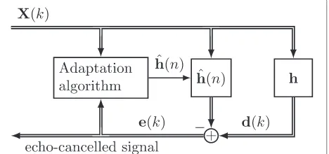
In this section, the system identification problem is related to AEC, and the signal model is introduced along with Fig. 1.
In the following, theLloudspeaker signals are described by the matrix X(k) which captures the individual sam-plesxl(k)of loudspeaker channell(l= 0, 1,. . .,L−1) at discrete-time instantk. The structure of this matrix will
be explained and motivated later. These signals are fed to the LEM system, which is represented by the vector hthat captures the impulse responses of all microphone-to-loudspeaker paths. The LEM system is assumed to be time-invariant for the subsequent analysis. The individ-ual samples of the impulse response from loudspeaker l to microphonem(m = 0, 1,. . .,M−1) are denoted by hm,l(k)such that microphone signalmis given by
dm(k)= L−1
l=0 K−1
κ=0
xl(k−κ)hm,l(κ). (1)
This implies that the LEM system impulse responses are considered to be of lengthKand that additive noise in the microphone signals is neglected. Although these condi-tions will not be fulfilled for real-world systems, this does not limit the applicability of the following derivation.
The discrete-time microphone signals are captured by the vector
d(k)=(d0(k),d1(k),. . .,dM−1(k))T, (2)
dm(k)=(dm(k−P+1),. . .,dm(k))T, (3)
where signal segments of length P are considered and ·T denotes the transposition. The choice of P will be discussed later. For system identification, an adaptation algorithm provides an estimatehˆ(n)ofh. Typically, this estimate is determined implicitly by minimizing a given norm of the error signal e(k). In the echo cancellation context, the error signale(k)contains also the signals of the local sources in the LEM system, which should then be further processed and/or transmitted after the acoustic echoes are removed.
The column vectorhˆ(n) of lengthKLM has the same structure ashbut is dependent on the block-time index n= k/N, whereNdenotes the frame shift of the adap-tation algorithms as defined later and·denotes the floor operator. The resulting structure ofhˆ(n)is then given by
ˆ h(n)=
ˆ
hT0,0(n),hˆT0,1(n),. . .,hˆT0,L−1(n),
ˆ
hT1,0(n),. . .,hˆTM−1,L−1(n)T
(4)
ˆ
hm,l(n)=
ˆ
hm,l(0,n),. . .,hˆm,l(K−1,n)T, (5)
wherehˆm,l(k,n)are estimates ofhm,l(k).
In order to implement (1) by the multiplication
d(k)=X(k)h, (6)
theMP×LMKmatrixX(k)has to be defined as follows. The loudspeaker signals are first represented by
xl(k)=(xl(k−P+1),. . .,xl(k))T, (7)
which is then used to form
Xl(k)=(xl(k),. . .,xl(k−K+1)), (8)
such that
X(k)=IM⊗(X0(k),X1(k),. . .,XL−1(k)), (9)
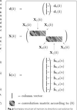
can be defined. Here, ⊗ denotes the Kronecker prod-uct, andIMis anM×Midentity matrix. The redundant representation of X(k) in (9), as illustrated by Fig. 2, allows for describing the microphone signalsd(k)as a col-umn vector. This representation will be exploited later in Section 5.
The adaptation error signal is then defined by
e(k)=d(k)−X(k)hˆ(n). (10)
Note thatk may assume any integer number, while only the time instants k = nN will be relevant for the derivation of the adaptation algorithms presented later. In real-world implementations,e(k)will be used for further processing, which suggests to set the microphone signal segment lengthPequal to the frame shift N to obtain a gap-less signal in e(k). However, for generality, P is not determined byNin the presented derivation.
Fig. 2Exemplary structure of matrices to describe a convolution for
When minimizing the mean-square error (MSE), i. e., solving
argmin ˆ h(n)
EeH(k)e(k) (11)
with·H denoting the Hermitian transpose, the following normal equation results:
Rhˆ(n)=r, (12)
with
R=EXH(k)X(k), (13)
r=EXH(k)d(k) (14)
being scaled versions of the loudspeaker signal autocor-relation matrix and the cross-corautocor-relation vector of loud-speaker and microphone signals, respectively. The scaling results from theProws ofXl(k), which are time-shifted versions of each other. Since stationarity implies shift invariance under the expectation operator,Rrepresents the sum ofPidentical loudspeaker signal autocorrelation matrices. The same holds forrwith respect to the cross-correlation vector. IfP=1 is chosen,Randrdescribe the loudspeaker signal autocorrelation matrix and the cross-correlation vector of loudspeaker and microphone signals, respectively, as they are commonly used in the literature [17].
3 Recursive least-squares (RLS) and least-mean-square (LMS) algorithms
In the first part of this section, the well-known RLS algorithm is briefly reviewed to form the basis for the subsequent derivations. In Section 3.1, the effect of fil-ter coefficient errors on the further convergence of the RLS algorithm is treated. The LMS algorithm is derived in Section 3.2 in order to establish a link between the LMS algorithm and a Tikhonov regularization of the RLS algorithm.
The RLS algorithm as considered here minimizes the cost function
JRLS(n)= n
ν=0
λn−νeH(νN)e(νN), (15)
using the exponential window defined by “forgetting fac-tor”λ[17]. The weighted least-squares criterion given by (15) approximatesEeH(k)e(k)in (11) and can be used when the second order moments of the loudspeaker and microphone signals are unknown. When choosingN = P = K, (15) is identical to the cost function used in [39] up to a scaling factor.
Plugging (10) into (15) and setting the Wirtinger gra-dient [17, 46] of the result to zero leads to anhˆ(n) that minimizes (15). This gradient is given by
∂JRLS(n) ∂hˆH(n) =
n
ν=0
λn−νXH(νN)X(νN)hˆ(n)−XH(νN)d(νN),
(16)
where ∂
∂hˆH(n)JRLS(n)=0 leads to ˆ
R(n)hˆ(n)= ˆr(n) (17)
with
ˆ R(n)=
n
ν=0
λn−νXH(νN)X(νN) (18)
=λRˆ(n−1)+XH(nN)X(nN), (19)
ˆ r(n)=
n
ν=0
λn−νXH(νN)d(νN) (20)
=λrˆ(n−1)+XH(nN)d(nN). (21)
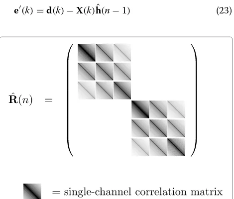
Note thatRˆ(n)andˆr(n)can be seen as recursive estimates ofRandr, respectively, such that (17) approximates the solution defined by (12). Due to the similarity between (13) and (18), Rˆ(n) shares the structure of R, which is illustrated in Fig. 3.
In the following, a recursive algorithm determininghˆ(n) is derived. Multiplying (19) from the right-hand side by the previously computed filter coefficientshˆ(n−1)and subtracting the result from (21) leads to
ˆ
r(n)− ˆR(n)hˆ(n−1)=λrˆ(n−1)− ˆR(n−1)hˆ(n−1)
+XH(nN)d(nN)−X(nN)hˆ(n−1). (22)
Substituting rˆ(n) using (17) and defining the a priori estimation error
e(k)=d(k)−X(k)hˆ(n−1) (23)
leads to
ˆ
R(n)hˆ(n)= ˆR(n)hˆ(n−1)+XH(nN)e(nN)
+λrˆ(n−1)− ˆR(n−1)hˆ(n−1) (24)
and finally to the explicit formulation of the adaptation algorithm, assuming thatRˆ(n)is invertible andhˆ(n−1) fulfills (17) forn−1:
ˆ
h(n)= ˆh(n−1)+ ˆR−1(n)XH(nN)e(nN). (25)
Note that the a priori estimation error e(k) must be clearly distinguished from the a posteriori estimation error e(k), which depends onhˆ(n) instead of hˆ(n− 1). Unfortunately, these errors are not correctly distinguished in [39].
Since (17) describes the solution of a least-squares prob-lem,Rˆ−1(n)can be replaced by the Moore-Penrose pseu-doinverse, ifRˆ(n)is not invertible [17]. However, this is merely of theoretical interest since the Moore-Penrose pseudoinverse is expensive to compute, and real-world implementations will most likely rely on regularization as described later by (36). Moreover, the inverseRˆ−1(n) can also be computed using the well-known matrix inver-sion lemma [17]. However, this approach leads only to an increased efficiency, if (19) describes a rank-deficient update ofRˆ(n), where a higher rank of the update implies a lower gain in efficiency. Hence, this approach is less attrac-tive with growingP. Additionally, the update of the matrix inverted in (36) is generally full-rank. Thus, this approach is not discussed in the paper.
3.1 Effect of regularization and approximation errors For any approximation or regularized version of the RLS algorithm, (17) will not be fulfilled exactly by hˆ(n− 1). In that case, λrˆ(n−1)− ˆR(n−1)hˆ(n−1) does not
vanish, andhˆ(n−1)can be described by
ˆ
h(n−1)= ˆhopt(n−1)+hˆ(n−1), (26)
where the optimal componenthˆopt(n−1)of the filter coef-ficients fulfills (17) at block time instantn−1, while the error componenthˆ(n)does not. Then, multiplying (24) withRˆ−1(n)from the left-hand side leads to
ˆ
h(n)= ˆh(n−1)+ ˆR−1(n)XH(nN)e(nN)
+λRˆ−1(n)
ˆ
r(n−1)− ˆR(n−1)hˆ(n−1)
(27)
as the adaptation rule to obtain optimal filter coefficients from previous suboptimal coefficients. When comparing (25) to (27) it can be seen that suboptimal filter coeffi-cientshˆ(n−1) require an additional correction term in order to obtain optimal coefficients in hˆ(n). Since this term is not considered in (25), any perturbation ofhˆ(n−1)
will lead to suboptimal coefficients in hˆ(n). The result-ing error can be determined by subtractresult-ing (25) from (27) and plugging (26) into the result. Then,ˆr(n−1)− ˆR(n− 1)hˆopt(n−1)vanishes, which leads to
hˆ(n)= −λRˆ−1(n)Rˆ(n−1)hˆ(n−1). (28) This gives rise to the question how this error propagates in the following iterations. Fortunately, recursive application of (28) leads to
hˆ(n+1)=(−λ)2Rˆ−1(n+1)Rˆ(n−1)hˆ(n−1), (29) hˆ(n+2)=(−λ)3Rˆ−1(n+2)Rˆ(n−1)hˆ(n−1),
(30)
which shows that any error introduced in hˆ(n) decays exponentially, while the reconvergence speed is deter-mined by the parameterλ.
3.2 Link between the LMS algorithm and the Tikhonov regularized RLS algorithm
To establish the link between the LMS algorithm and the regularized RLS algorithm, the LMS algorithm is briefly derived in the following. To this end, solving (11) using the gradient descent method can be viewed as a first step [17]. In that approach, the filter coefficientshˆ(n)are deter-mined computing the gradient of EeH(nN)e(nN)for
ˆ h(n−1),
ˆ
h(n)= ˆh(n−1)+μr−Rhˆ(n−1), (31)
whereμis a parameter to control the step size that could also be set adaptively [35]. For simplicity, the LMS algo-rithm uses the instantaneous estimates of (13) and (14) given by
R≈XH(k)X(k), (32)
r≈XH(k)d(k). (33)
This leads to a representation of (31) by ˆ
h(n)= ˆh(n−1)+μXH(nN)
·d(nN)−X(nN)hˆ(n−1)
, (34)
= ˆh(n−1)+μXH(nN)e(nN), (35) where (23) was used to obtain (34) from (35). While choosingP = N = 1, (35) describes the LMS algorithm in its most common form, the formulation presented here allows for block-wise processing of the data.
When comparing (35) to (25), structural similarities can be exploited to obtain the following equation:
ˆ
h(n)= ˆh(n−1)+
(1−α)Rˆ(n)+α
μIKLM
−1
XH(nN)e(nN),
whereαis a parameter of choice with 0≤α≤1. Forα = 0, (36) describes the RLS algorithm (25), for α = 1, the LMS algorithm (35) is described. By choosingαbetween 0 and 1, the adaptation steps can be continuously varied in between both algorithms, although the relation is not lin-ear. SinceRˆ(n)is positive semi-definite, the inverse exists for any α > 0. Moreover, when computing the inverse, choosing a largerαcan reduce the condition number of the matrix to be inverted.
A comparable consideration can be found in [47]. How-ever, the block RLS algorithm used there does only con-sider the current data block and does not allow for an exponential time-windowing. Furthermore, the NLMS algorithm described there is identical to the algorithm that is most commonly referred to as affine projection algo-rithm. In [47], it is not possible to continuously vary the relative weight of the adaptation steps provided by both algorithms.
4 Generalized frequency-domain adaptive filtering algorithm
The derivation of the GFDAF algorithm presented in this section differs from [39] in the following points:
• The derivation is based on replacing the convolution matrices captured in (25) by DFT-domain
multiplication instead of defining an equivalent to (15) in the DFT domain. This allows to show the relation of the GFDAF algorithm to the RLS
algorithm more clearly. A similar approach is known for the Kalman filter-based AEC [14, 36].
• An erroneous equality used in the original derivation is clearly identified as an approximation.
• The frame shiftNand the lengths of the adaptive filtersK can be chosen independently of the
microphone signal segment lengthP, as it was already described for the single-channel frequency-domain adaptive filtering algorithm [4] and for the Kalman filter implementations in the DFT-domain [14, 36, 43].
• The multichannel microphone signals are represented by a vectord(k)instead of a matrix, which allows for considering simplified models, as described later. • A different regularization approach is proposed that
is closely linked to the well-known LMS algorithm.
In [39], a DFT-domain equivalent to (15) was used to derive the GFDAF algorithm. Since the block RLS algo-rithm derived in (3), which minimizes (15) involves no approximations, (25) can be used for further derivations without restrictions. As a first step, (25) will be rewrit-ten in the DFT domain such that this representation can be approximated to formulate the GFDAF algorithm. It is well-known that a time-domain convolution can
be facilitated by a DFT-domain multiplication using the overlap-save method [14, 36]. This approach is described in the following to ensure compatibility with the notation used in this paper, aiming at a length-QDFT-domain rep-resentation of the loudspeaker signals captured in X(k). First, the individual loudspeaker signalsXl(k)are consid-ered, where
Xl(k)= 0P×(Q−P),IP ˚
Xl(k)
IK 0(Q−K)×K
(37)
with
˚
Xl(k)=
X(lA)(k) X(lB)(k) Xl(k) X(lC)(k)
(38)
holds for any matrices X(lA)(k), Xl(B)(k), and X(lC)(k) of compatible dimensions. SinceXl(k)is a Toeplitz matrix, X(lA)(k), Xl(B)(k), and X(lC)(k) can be chosen such that
˚
Xl(k)is a circulant matrix that can be diagonalized by the DFT matrix. The entries of theQ×QDFT matrixFQin rowpcolumnqare given by
FQ
p,q=
1 √
Qe
−j(p−1) (q−1)2π
Q, (39)
where j is used as the imaginary unit. The symmetric definition of the DFT using the scaling factor 1/√Qin (39) is crucial for the following considerations, although a different scaling factor was used in [39]. This leads to
Xl(k)=FQX˚l(k)FHQ (40)
=QDiagFQxl(k)
(41)
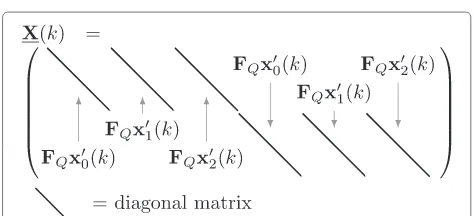
where xl(k) is defined like xl(k) but capturing signal segments of lengthQinstead ofP. To describe the filter-ing through a multiple-input/multiple-output system, the individual matricesXl(k)are captured by
X(k)=IM⊗ X0(k),X1(k),. . .,XL−1(k), (42)
as it is also described by [39, 43]. The structure ofX(k)is illustrated in Fig. 4.
UsingX(k), it is possible to write
X(k)=W01X(k)W10, (43)
Fig. 4Structure of the DFT-domain loudspeaker signals forL=3,
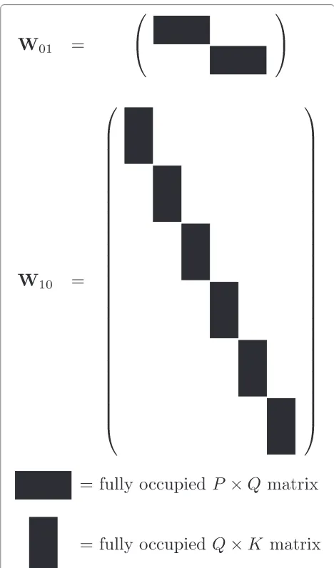
where the matrices
W01=IM⊗ 0P×(Q−P),IP
FHQ
, (44)
W10=ILM⊗
FQ
IK 0(Q−K)×K
(45)
are used to transform signal vectors from and to the DFT domain as well as for discrete-time truncation and zero-padding operations. An example for the structure of the matrices described by (44) and (45) is shown in Fig. 5. Note thatQ=P+K−1 is not necessary following, but Q≥P+K−1 is assumed. This is different to [39], where only the caseQ=2P=2Kwas covered.
For the further derivations,
ˆ
S(n)=λSˆ(n−1)+XH(nN)WH01W01X(nN) (46)
Fig. 5Structure of the windowing matrices forL=3,M=2
is defined, where (43) and (19) can be used to verify that ˆ
R(n)=WH10Sˆ(n)W10 (47)
holds. The matrixSˆ(n)can be interpreted as an estimate of the DFT-domain power spectral density of the loud-speaker signals. Considering (25) and replacingRˆ(n) by (47) andXH(nN)by (43) results in
ˆ
h(n)= ˆh(n−1)+WH10Sˆ(n)W10
−1
·WH10XH(nN)WH01e(nN),
(48)
which represents the same time-domain update equation as (25) but is based on DFT-domain representations of the involved signalsX(k)ande(k).
In (48), the size of the generally fully occupied matrix WH10Sˆ(n)W10and its inverse preclude a real-world imple-mentation of this algorithm for larger filter lengths or a larger number of loudspeaker channels. To overcome this obstacle, it was proposed in [39] to invert a sparse approximation ofSˆ(n)rather than invertingWH10Sˆ(n)W10 in (48).
As X(k) is sparse, the lack of sparsity in Sˆ(n) can be attributed to the term WH01W01 which represents win-dowing with a rectangular window in the time domain. Considering the definition of the DFT matrix given by (39), evaluatingWH01W01leads to
WH01W01=IM⊗
FQDiag{w}FHQ
, (49)
with
FQDiag{w}FHQ
ζ,η= 1 Q
Q−1
k=0
w(k) ejk(η−ζ )2Qπ, (50)
wherew(k)describes an appropriate rectangular window function with the vector representation
w=(w(0),w(1),. . .,w(Q−1))T. (51)
Forw(k) = 1, (50) would describe an identity matrix, while the definition of
w(k)=
1 forQ−P≤k<Q,
0 otherwise (52)
describes the time-domain windowing according to (44). As described in [39], (50) can be identified as a finite geometric series, which allows to write (52) as
FQDiag{w}FHQ
ζ,η
= ⎧ ⎨ ⎩ P
Q forζ =η
−1 Q ·1−e
j(Q−P)(η−ζ )2π
Q
1−ej(η−ζ )2Qπ
otherwise. (53)
shift or asymmetry of the window in each row. The max-imum of this function is located on the main diagonal, which suggests an approximation ofWH01W01by an iden-tity matrix. The approximation tends to be more accu-rate, the narrower the main lobe of the sinc function is or, equivalently, the larger the time-domain window is. Hence,WH01W01 can be better approximated by a scaled identity matrix the largerPis, where
WH01W01≈IMQP
Q. (54)
This is an important generalization relative to [39], since Pis a parameter of choice in contrast to [39], where only the special caseQ = 2Pwas considered. Note that the same result was already obtained for the Kalman filter implementations in the DFT-domain [14, 36, 43].
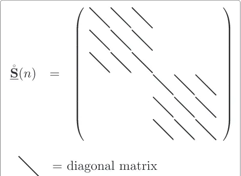
Using (54), (46) can be approximated by
˚
S(n)=λS˚(n−1)+ P QX
H(nN)X(nN) (55)
where the structure ofS˚(n)is illustrated in Fig. 6. Replac-ing Sˆ(n) by S˚(n) in (48) does not lead to an obvious advantage, yet. Therefore, another approximation is used:
WH10S˚(n)W10
−1
≈WH10S˚−1(n)W10, (56)
whereS˚−1(n)is now the inverse of a sparse matrix that is inexpensive to compute when exploiting the matrix struc-ture accordingly. Erroneously, (56) was not identified as an approximation in [39] but as an equality. This is discussed in Appendix A, where using (56) is also justified.
Eventually, (56) can be used to approximateRˆ−1(n)in the DFT-domain, which distinguishes the GFDAF algo-rithm from the RLS algoalgo-rithm. Not only that this leads to tremendous computational savings, it also decouples the adaptation of the individual DFT bins [39]. As a result,
Fig. 6Illustration of the structure of the matrix˚S(n)forL=3,M=2
there areQ-independent inverses ofL×Lmatrices to be determined, instead of the inverse of oneLK×LKmatrix. This explains the robustness of this algorithm, which is described by:
ˆ
h(n) = ˆh(n−1)+μWH10
˚
S(n)+D(n)
−1
W10
≈ ˆR−1(n) ·WH10XH(nN)WH01e(nN)
=XH(nN)e(nN)
, (57)
where the step-size parameter μ can be viewed as accounting for the inaccuracy of the approximation. This allows for using a step size close to or even larger thanμ= 1, according to the needs of the considered application scenario. Furthermore, the matrix
D(n)=(n)IKLM (58)
is used for regularization which is generally necessary for real-world implementations since S˚(n) will typically exhibit a large condition number or even become singular for signalsX(k)with small spectral flatness or when the loudspeaker signals are strongly correlated.
A straightforward approach is to use a regularization weight function that is proportional to the loudspeaker signal power as defined by
(n)=λ(n−1)+ δP LQ
L
l=1
xHl (nN)xl(nN), (59)
For efficient implementations, it is common to imple-ment the time-domain convolution in the DFT domain. Accordingly, the a priori error signal can be expressed by
e(k)=d(k)−W01X(k)W10hˆ(n−1). (60)
Any multiplication withW10 impliesLM DFTs, while a multiplication withW01impliesMDFTs. To decrease the computational demands, four multiplications byW10can be eliminated by approximations. First,W10WH10 can be approximated in the same way asWH01W01by
W10WH10≈ILMQ K
Q, (61)
whereKhas the same role asPin (54). In (57), this leads to
ˆ
h(n) = ˆh(n−1)+μK QW
H 10
˚
S(n)+D(n)−1
·XH(nN)WH01e(nN), (62) where the time-domain windowing byW10WH10is omit-ted. Furthermore, when considering
ˆ
h(n)=W10hˆ(n), (63)
the matrixWH10 can also be neglected which leads to the so-called unconstrained variant [39, 41] of this algorithm given by
ˆ
h(n)= ˆh(n−1)+μK Q
˚
S(n)+D(n)−1XH(nN)WH01e(nN).
(64)
In that case, (60) is also simplified to
e(k)=d(k)−W01X(k)hˆ(n−1). (65)
The time-domain windowing operations applied to the error signal cannot be neglected for the definition of the algorithm. Otherwise, the adaptive filter would converge to a solution for cyclic convolution and not to a solu-tion for linear convolusolu-tion with the time-domain filter coefficients.
5 Pruned loudspeaker-enclosure-microphone models
In this section, the adaptation algorithms described above are generalized to allow for system identification or AEC using pruned LEM models. Considering the structure of
ˆ
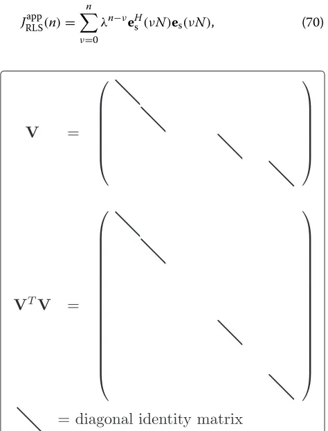
h(n)described in (4), it is possible to define a matrixV that implies certain components inhˆ(n)to be zero. This is done by requiring
VTVhˆ(n)= ˆh(n) (66)
within this section, which implies that certain coefficients inhˆ(n)are zero. Note that this is the only definition nec-essary to generalize the considered adaptation algorithms to pruned LEM models.
The values ofVcan be defined by
VTV=Diag{v}, (67)
where componentζ of the vectorvis given by
[v]ζ =
1 if [h]ζis modeled,
0 otherwise. (68)
At the same time, a multiplication byVfrom the left-hand side would prune the zero-valued coefficients fromhˆ(n). Exemplary structures ofVandVTVare shown in Fig. 7. Note that the following derivation of the RLS algorithm allows to choose freely whether any of the coefficients of h is modeled or not. This comprises the simplified model proposed in [45], but it would also allow for choos-ing individual impulse response lengths for each modeled loudspeaker-to-microphone path. However, the deriva-tion of the GFDAF algorithm in Sec. 4 is based on DFTs of the same lengths, which precludes choosingv arbitrar-ily. Hence, for the GFDAF, it is only possible to model either all or none of the coefficients describing a certain loudspeaker-to-microphone path.
To derive an adaptation algorithm for pruned models, the error signal (10) must be modified according to
es(k)=d(k)−X(k)VTVhˆ(n). (69)
For the RLS algorithm, this results in the cost function
JRLSapp(n)= n
ν=0
λn−νeHs (νN)es(νN), (70)
where the derivation of the adaptation algorithm uses exactly the same steps as shown above. Consequently, considering the derivation above, while replacinghˆ(n)by Vhˆ(n) andX(k) by X(k)VT results in the desired algo-rithm. The latter replacement implies a further replace-ment ofRˆ(n)byVRˆ(n)VT.
At this point, a definition of the a priori estimation error for pruned LEM models might be expected, which would then be used instead of e(nN). However, this is not necessary since (71) already implies that all unmodeled coefficients are set to zero inhˆ(n). It can be seen from (71) that the dimensions of the involved inverse can be reduced when using pruned models.
Multiplying (71) by VT from the left-hand side and requiring
which is implied by (66), leads to an explicit formulation of the algorithm given by
ˆ
For pruned models, the gradient descent approach described in (31) is given by
ˆ
Plugging (32) and (33) into (74) results in the LMS update ˆ
h(n) = ˆh(n−1)+μVTVXH(nN) ·d(nN)−X(nN)VTVhˆ(n−1)
, (75)
where (23) and (66) can be used to formulate the LMS algorithm for pruned models:
ˆ
h(n)= ˆh(n−1)+μVTVXH(nN)e(nN). (76)
As the GFDAF algorithm approximates the RLS algo-rithm, the formulation of the RLS algorithm for simplified models can be straightforwardly translated to obtain
ˆ
by comparing (57) and (73). Note that the termVTVcan be omitted as along ashˆ(n−1)fulfills (66). The formula-tions of (62) and (64) can be obtained in the same manner, where (64) requires a redefinition of V to consider the doubled number of coefficients inhˆ(n), compared tohˆ(n).
When comparing (73), (77), and (75) to (36) and (57), it can be seen that the relation of the regularized GFDAF algorithm to the LMS algorithm can also be established for simplified LEM models.
6 Evaluation results
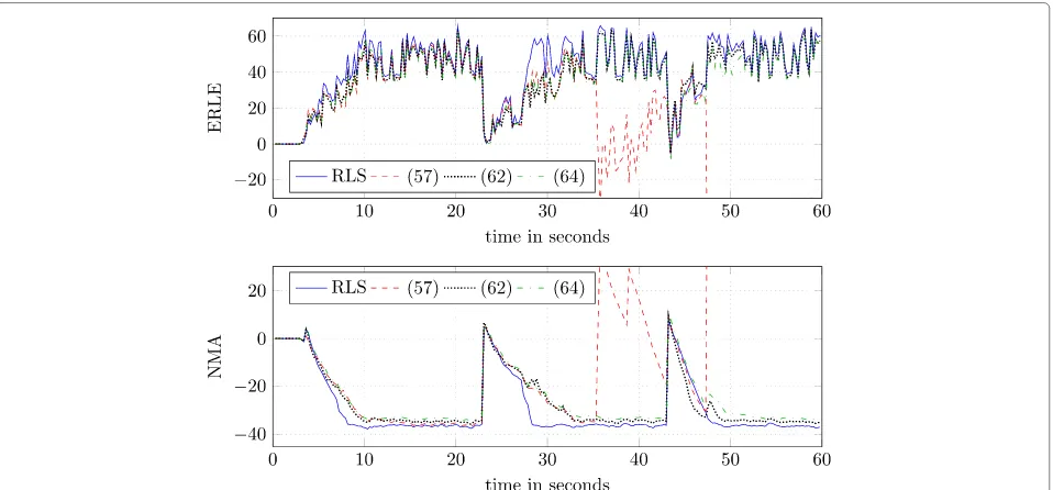
In this section, a brief experimental evaluation of the treated adaptation algorithms is presented. This evalua-tion is focused on the effects of the approximaevalua-tions used in the derivation of the GFDAF algorithm. Hence, the RLS algorithm given by (25) is compared to the three pre-sented variants of the GFDAF algorithm, given by (57), (62), and (64). To this end, the following AEC scenario is considered: two loudspeaker signals (L=2) carry a stereo recording of a speech signal superimposed by mutually uncorrelated white Gaussian noise signals such that a signal-to-noise ratio (SNR) of 20 dB results on average. This rather low SNR was chosen to avoid using a regular-ization in the first two experiments that would otherwise obscure insights into the influence of the approximations used for the GFDAF algorithm. From the loudspeaker sig-nals, two microphone signals (M=2) have been obtained through convolution with four impulse responses, mea-sured in a room with a reverberation timeT60of approxi-mately 0.36 s.
Using a sampling frequency of 8 kHz, the impulse responses were truncated to 128 samples such that the adaptive filters could, in theory, perfectly model the impulse responses with the chosenK = 128. This choice was imposed by the large computational demands of the RLS algorithm. To simulate microphone noise, mutually uncorrelated white Gaussian noise signals were added to the microphones such that a signal-to-noise ratio of 40 dB results on average.
The three experiments last for a simulated time span of 60 s, where no adaptation is performed during the first 3 s in order to obtain sufficiently well-conditioned matrices
ˆ
ERLE(n)=20 log10
d(nN)2 e(nN)2
, (78)
where ·2 denotes the Euclidean norm. Note that the actual microphone signal was only used for the adaptation of the filters, while the noise-free microphone signal was used to determine the ERLE. This measure was termed “true ERLE” in [48] and allows to assess the echo cancella-tion performance also during perturbacancella-tion. On the other hand, the NMA is defined by
NMA(n)=20 log10
ˆh(n)−hF hF
, (79)
where·Fdenotes the Frobenius norm and measures the system identification accuracy.
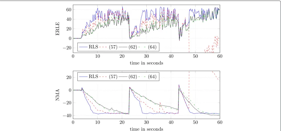
The results of this experiment can be seen in Fig. 8, whereλ = 0.99,μ = 1,K = 128,P = 128,Q = 256, and N = 64 have been chosen for all algorithms (if applicable). It can be seen that the RLS algorithm shows the best performance in terms of ERLE and NMA. This is an expected result since it uses no approximations. It can be furthermore seen that the approximation intro-duced with the algorithm described by (57) leads to a slower convergence. The approximations used for (62) leads to a further reduction in convergence speed, while the algorithm described by (64) shows nearly an identical performance compared to using (62). It can be seen that the reconvergence behavior after the impulse response change and the perturbation of the microphone signal is very similar to the initial convergence. However, it can be seen that the algorithm described by (57) shows a low
robustness at some time instants. Note that the break-down in ERLE and NMA that exceed the scale of the plot reach up to−100 and 100 dB, respectively. After that, a stable reconvergence can be seen. An explanation for this sudden breakdown can be found when considering (55) in conjunction with (62), which describes a GFDAF variant that does not exhibit this property. It can be shown that
˚
S−1(n)XH(nN) (80)
yields a matrix with entries that are weighted inversely proportional to the weights of the corresponding entries inXH(nN). This is becauseXH(nN)is also considered in
˚
S(n), while all DFT bins are decoupled. However, when considering
˚
S−1(n)W10WH10XH(nN), (81)
as implied by (57), the DFT bins are no longer decou-pled because of the time-domain windowing byW10WH10. Thus, it is possible that a sharp spectral peak in X(nN) leaks into the neighboring bins in the product W10WH10XH(nN). On the other hand, S˚−1(n) does not describe a time-domain windowing, which implies that a sharp spectral peak in X(nN) will not not be spread inS˚(n). Due to this mismatch, the entries in the matrix resulting from (81) can exhibit a relatively strong weight, which implies larger adaptation steps and can lead to problems in some cases.
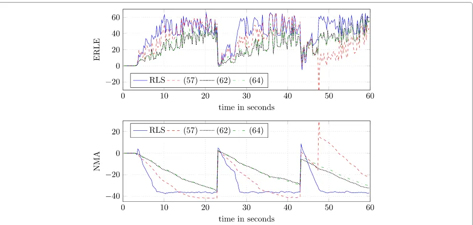
While comparing the considered algorithm using iden-tical parameters for all of them allows to investigate the properties of the individual algorithms, it is not a fair per-formance comparison. Hence, an optimal step sizeμfor
the variants of the GFDAF algorithm was determined by subsequent increasingμuntil no further improvement in ERLE was noticeable. The optimal step sizes determined for (57), (62) and, (64) were μ = 1.2, μ = 3.1, and μ = 2.4, respectively. This is actually a surprising result since approximations typically call for a more conserva-tive step size. For performance evaluation, the experiment described above was repeated using these step sizes, while all other parameters were kept. The results presented in Fig. 9 show that all variants of the GFDAF algorithm are able to approach the performance of the RLS algorithm, which is shown for comparison. As expected, the robust-ness of the algorithm described by (57) is obviously even more reduced whenμis increased.
In Fig. 10, the experiment described for Fig. 8 was repeated, were the variants of the GFDAF algorithm have been regularized, while the RLS algorithm was not reg-ularized to allow for a comparison. As explained above, larger values of δ will result in adaptation steps of the GFDAF algorithm that are closer to the adaptation steps the LMS algorithm would provide. Since the GFDAF algorithm is superior to the LMS algorithm in terms of convergence speed, δ should be chosen as low as pos-sible. As the algorithms described by (62) and (64) do not depend strongly on a regularization in the considered scenario, δ = 0.03 was chosen. This choice represents a compromise between the optimum regularization of the algorithm described by (57) and not hampering the convergence of the other algorithms.
As expected, the convergence speed of the all regular-ized algorithms is slightly reduced, while the impact of the impulse in the microphone signal is also slightly reduced
by the regularization. The most interesting results are those for the algorithm described by (57). While the reg-ularization mitigates the robustness problem, it is not able to prevent the divergence completely. At the same time, the NMA achieved by this algorithm during nor-mal convergence of this algorithm is improved, such that it achieves a better system identification than the RLS algorithm. Note that the RLS is optimal with respect to increasing ERLE, but not necessarily optimal to decrease the NMA, as it would be the case for the Kalman filter-based approaches.
Results of an evaluation with a varied microphone-signal segment size are not presented as the effect of varying thePwas only marginal in the considered experi-mental scenario.
7 Real-world implementations of the GFDAF algorithm
In this section, some notes on the implementation of the GFDAF algorithm are given. The most attractive vari-ants for implementation of this algorithm are given by (62) and (64), as also proposed in [39]. In both cases, the
term
˚
S(n)+D(n)
−1
XH(nN) needs to be computed. Considering the dimensions of the involved matrices, it becomes clear that a real-world implementation must exploit sparsity in order to be feasible. The structures of the relevant matrices are illustrated in Figs. 4 and 6 and can be considered straightforwardly. For computing
˚
S(n)+D(n)−1XH(nN), all DFT-bins can be treated independently, which allows for a straightforward paral-lelization of the algorithm. This can be beneficial for the
Fig. 10ERLE and NMA for an AEC experiment with regularized algorithms
implementation of the algorithm on multi-core proces-sors [49]. Since
˚
S(n)+D(n)
is positive semi-definite, it is possible to use the Cholesky decomposition for an efficient computation.
Still, forM> 1, the definition (42) implies redundancy inX(k)that is propagated intoS˚(n)such that it appears as if the derivation given above would not describe an efficient implementation. Equation 55 in conjunction with (42) and the well-known identity
AC⊗BD=(A⊗B) (C⊗D) (82)
can be used to show thatS˚(n)can also be obtained by
˚
S(n)=IM⊗S˚(n), (83)
whereS˚(n)is equal toS˚(n)forM = 1. Additionally, the Kronecker product has the property
(A⊗B)−1=A−1⊗B−1, (84)
which implies that this redundancy does not increase the computational effort for invertingS˚(n). Finally, the cost
of computing
˚
S(n)+D(n)
−1
XH(nN) dominates the overall effort and is proportional toQL3. When accepting some restrictions on the regularization, this value may be reduced toQL2[39]. While this constitutes a considerable effort, it has to be considered that the RLS algorithm (25) would imply a computational effort proportional to(KL)2, noting that typicallyK,QL.
When considering the term
V
˚
S(n)+D(n)
VT
in (77), it can be seen that (83) and (84) are not gen-erally applicable to determine its inverse. Thus, care
must be taken that V reduces the matrix dimensions sufficiently such that a computational advantage is achieved compared to general models. It has been shown that WDAF allows for sufficiently simplified models to decrease the computational demands [45]. When coupling W wave-domain loudspeaker signals to each wave-domain microphone signal, the cost of comput-ing V
˚
S(n)+D(n)VT
VXH(nN) is proportional to QW3M, which implies computational savings whenever W3M < L3. A value ofW = 3 is already sufficient for many application scenarios [45].
8 Conclusions
convergence speed, while some robustness issues still have to be solved. This can be an avenue for future research.
Appendix A: Approximating the inverse of a power spectral density matrix
For the derivation of the GFDAF algorithm, the following approximation is crucial:
Unfortunately, (85) was mistaken for an equivalence in [39], and it was claimed that multiplying Sˆ(n)W10 from the right-hand side would prove this. However,Sˆ(n)W10 is a singular matrix which invalidates this proof. In the fol-lowing, (85) is analyzed for the caseL=M=1,Q=2K, which is chosen for the sake of brevity and can be straight-forwardly extended to scenarios with different L,M,Q, andK.
Since the dimensions of Sˆ(n) are larger than those of ˆ tively, (40) and (44) can be used to obtain
ˆ
To determine the inverse of R2ˆ (n) , the block-matrix inversion can be used. It is given by
whereA,B,C, andDare arbitrary matrices of compatible dimensions. ConsideringW10WH10 in (85), it is clear that onlyAandBare relevant in our case, which are given by describes the cross-correlation between both. Assum-ing that Rˆ(n) and RˆCC(n) are well-conditioned, while their entries exhibit significantly stronger weights than those in RˆC(n), the terms RˆC(n)Rˆ−1CC(n)RˆHC(n) and
ˆ
RHC(n)Rˆ−1(n)RˆC(n) are of no importance. Hence, A approximates Rˆ−1(n) while the influence ofB is small, which justifies the use of (85) as an approximation.
Abbreviations
AEC: acoustic echo cancellation; DFT: discrete Fourier transform; ERLE: echo return loss enhancement; GFDAF: generalized frequency-domain adaptive filtering; IPNLMS: improved proportionate normalized least-mean squares algorithm; LEM: loudspeaker-enclosure-microphone; LMS: least mean square; MSE: mean square error; NLMS: normalized least-mean-square; NMA: normalized system misalignment; PNLMS: proportionate normalized least-mean-squares algorithm; RLS: recursive least-squares; SNR: signal-to-noise ratio; WDAF: wave-domain adaptive filtering.
Competing interests
The authors declare that they have no competing interests.
Acknowledgements
Martin Schneider is currently with the Fraunhofer Institute for Integrated Circuits IIS, Germany.
Received: 30 June 2015 Accepted: 30 December 2015
References
1. E Hänsler, The hands-free telephone problem—an annotated bibliography. Signal Process.27(3), 259–271 (1992)
2. J Benesty, T Gänsler, DR Morgan, MM Sondhi, SL Gay,Advances in network and acoustic echo cancellation. (Springer, Berlin, Germany, 2001) 3. E Hänsler, G Schmidt,Acoustic echo and noise control: a practical approach.
(Wiley, Hoboken (NJ), USA, 2004)
4. P Vary, R Martin,Digital speech transmission: enhancement, coding and error concealment. (Wiley, Hoboken (NJ), USA, 2006)
5. E Hänsler, G Schmidt,Topics in acoustic echo and noise control: selected methods for the cancellation of acoustical echoes, the reduction of background noise, and speech processing. (Springer, Berlin, Germany, 2006) 6. MM Sondhi, inSpringer Handbook of Speech Processing. Adaptive echo
cancelation for voice signals (Springer, Berlin, Germany, 2008), pp. 903–928
7. G Enzner, H Buchner, A Favrot, F Kuech, inAcademic press library in signal processing: image, video processing and analysis, hardware, audio, acoustic and speech Processing, ed. by S Theodoridis, R Chellappa. Acoustic echo control, vol. 4 (Academic Press, Waltham (MA), USA, 2014)
8. SF Boll, Suppression of acoustic noise in speech using spectral subtraction. IEEE Trans. Acoustics, Speech and Signal Processing.27(2), 113–120 (1979) 9. C Faller, J Chen, Suppressing acoustic echo in a spectral envelope space.
IEEE Trans. Speech and Audio Processing.13(5), 1048–1062 (2005) 10. S Gustafsson, R Martin, P Vary, Combined acoustic echo control and noise
reduction for hands-free telephony. Signal Process.64(1), 21–32 (1998) 11. E Hänsler, GU Schmidt, Hands-free telephones–joint control of echo
cancellation and postfiltering. Signal process.80(11), 2295–2305 (2000) 12. S Gustafsson, R Martin, P Jax, P Vary, A psychoacoustic approach to
combined acoustic echo cancellation and noise reduction. IEEE Trans. Speech and Audio Processing.10(5), 245–256 (2002)
13. G Enzner, P Vary, inProc. European Signal Processing Conf. (EUSIPCO). New insights into the statistical signal model and the performance bounds of acoustic echo control (IEEE, Antalya, Turkey, 2005), pp. 1–4
14. G Enzner, P Vary, Frequency-domain adaptive Kalman filter for acoustic echo control in hands-free telephones. Signal Process.86(6), 1140–1156 (2006)
approach to residual echo suppression in robust hands-free teleconferencing (IEEE, Prague, Czech Republic, 2011), pp. 445–448 16. MM Sondhi, AJ Presti, A self-adaptive echo canceller. Bell Syst. Tech. J.
45(10), 1851–1854 (1966)
17. S Haykin,Adaptive filter theory. (Prentice Hall, Englewood Cliffs (NJ), USA, 2001)
18. E Hänsler,Statistische Signale: Grundlagen und Anwendungen. (Springer, Berlin, Germany, 2001)
19. K Ozeki, T Umeda, An adaptive filtering algorithm using an orthogonal projection to an affine subspace and its properties. Electron. Commun. in Japan (Part I: Communications).67(5), 19–27 (1984)
20. S Werner, JA Apolinário Jr, PSR Diniz, Set-membership proportionate affine projection algorithms. EURASIP J. Audio, Speech, and Music Processing.2007(1), 10–10 (2007)
21. SL Gay, S Tavathia, inProc. IEEE Intl. Conf. on Acoustics, Speech, and Signal Processing (ICASSP). The fast affine projection algorithm, vol. 5 (IEEE, Detroit (MI), USA, 1995), pp. 3023–3026
22. DL Duttweiler, Proportionate normalized least-mean-squares adaptation in echo cancelers. IEEE Trans. Speech and Audio Processing.8(5), 508–518 (2000)
23. J Benesty, SL Gay, inProc. IEEE Intl. Conf. on Acoustics, Speech, and Signal Processing (ICASSP). An improved PNLMS algorithm, vol. 2 (IEEE, Orlando (FL), USA, 2002), pp. 1881–1884
24. E Hänsler, inIEEE International Symposium on Circuits and Systems. Adaptive echo compensation applied to the hands-free telephone problem, vol. 1 (IEEE, New Orleans (LA), USA, 1990), pp. 279–282 25. C Breining, P Dreiseitel, E Hänsler, A Mader, B Nitsch, H Puder, T Schertler,
G Schmidt, J Tilp, Acoustic echo control. an application of very-high-order adaptive filters. IEEE Signal Proc. Mag.16(4), 42–69 (1999)
26. W Kellermann, Kompensation akustischer Echos in Frequenzteilbändern. Frequenz.39(7–8), 209–215 (1985)
27. W Kellermann, inProc. IEEE Intl. Conf. on Acoustics, Speech, and Signal Processing (ICASSP). Analysis and design of multirate systems for cancellation of acoustical echoes, vol. 5 (IEEE, New York (NY), USA, 1988), pp. 2570–2573
28. JJ Shynk, Frequency-domain and multirate adaptive filtering. IEEE Signal Process. Mag.9(1), 14–37 (1992)
29. P Sommen, P van Gerwen, H Kotmans, A Janssen, Convergence analysis of a frequency-domain adaptive filter with exponential power averaging and generalized window function. IEEE Trans. Circuits Syst.34(7), 788–798 (1987)
30. E Ferrara, Fast implementations of LMS adaptive filters. IEEE Trans. Acoustics, Speech, and Signal Processing.28(4), 474–475 (1980) 31. E Moulines, O Ait Amrane, Y Grenier, The generalized multidelay adaptive
filter: structure and convergence analysis. IEEE Trans. Signal Processing. 43(1), 14–28 (1995)
32. J-S Soo, KK Pang, Multidelay block frequency domain adaptive filter. IEEE Trans. Acoustics, Speech and Signal Processing.38(2), 373–376 (1990) 33. G Enzner, inProc. European Signal Processing Conf. (EUSIPCO). Bayesian
inference model for applications of time-varying acoustic system identification (IEEE, Aalborg, Denmark, 2010), pp. 2126–2130
34. Cn Paleologu, J Benesty, S Ciochina, Study of the general Kalman filter for echo cancellation. IEEE Trans. Audio, Speech, and Language Processing. 21(8), 1539–1549 (2013)
35. A Mader, H Puder, GU Schmidt, Step-size control for acoustic echo cancellation filters—an overview. Signal Process.80(9), 1697–1719 (2000) 36. F Kuech, E Mabande, G Enzner, inProc. IEEE Intl. Conf. on Acoustics, Speech,
and Signal Processing (ICASSP). State-space architecture of the partitioned-block-based acoustic echo controller, (2014), pp. 1295–1299 37. J Benesty, F Amand, A Gilloire, Y Grenier, inProc. IEEE Intl. Conf. on
Acoustics, Speech, and Signal Processing (ICASSP). Adaptive filtering algorithms for stereophonic acoustic echo cancellation, vol. 5 (IEEE, Detroit (MI), USA, 1995), pp. 3099–3102
38. J Benesty, DR Morgan, MM Sondhi, A better understanding and an improved solution to the specific problems of stereophonic acoustic echo cancellation. IEEE Trans. Speech and Audio Process.6(2), 156–165 (1998) 39. H Buchner, J Benesty, W Kellermann, ed. by J Benesty, Y Huang. Adaptive Signal Processing: Application to Real-World Problems (Springer, Berlin, Germany, 2003)
40. M Dentino, J McCool, B Widrow, Adaptive filtering in the frequency domain. Proc. IEEE.66(12), 1658–1659 (1978)
41. D Mansour, A Gray Jr., Unconstrained frequency-domain adaptive filter. IEEE Trans. Acoustics, Speech, and Signal Processing.30(5), 726–734 (1982)
42. J Benesty, P Duhamel, A fast exact least mean square adaptive algorithm. IEEE Trans. Signal Process.40(12), 2904–2920 (1992)
43. S Malik, G Enzner, Recursive Bayesian control of multichannel acoustic echo cancellation. IEEE Signal Process. Letters.18(11), 619–622 (2011) 44. H Buchner, S Spors, W Kellermann, inProc. IEEE Intl. Conf. on Acoustics,
Speech, and Signal Processing (ICASSP). Wave-domain adaptive filtering: acoustic echo cancellation for full-duplex systems based on wave-field synthesis, vol. 4 (IEEE, Montreal, Canada, 2004), pp. 117–120
45. M Schneider, W Kellermann, inProc. Joint Workshop on Hands-free Speech Communication and Microphone Arrays (HSCMA). A wave-domain model for acoustic MIMO systems with reduced complexity (IEEE, Edinburgh, UK, 2011), pp. 133–138
46. RFH Fischer,Precoding and signal shaping for digital transmission. (Wiley, Hoboken (NJ), USA, 2002)
47. M Montazeri, P Duhamel, A set of algorithms linking NLMS and block RLS algorithms. IEEE Trans. Signal Process.43(2), 444–453 (1995)
48. P Thune, G Enzner, inProc. Intl. Symposium on Image and Signal Processing and Analysis (ISPA). Trends in adaptive MISO system identification for multichannel audio reproduction and speech communication (IEEE, Berlin, Germany, 2013), pp. 767–772
49. M Schneider, F Schuh, W Kellermann, inITG-Fachbericht
Sprachkommunikation. The generalized frequency-domain adaptive filtering algorithm implemented on a GPU for large-scale multichannel acoustic echo cancellation (VDE, Braunschweig, Germany, 2012), pp. 39–42
Submit your manuscript to a
journal and benefi t from:
7Convenient online submission 7 Rigorous peer review
7Immediate publication on acceptance 7 Open access: articles freely available online 7High visibility within the fi eld
7 Retaining the copyright to your article