Study of Human Exposure Using Kriging Method
Ourouk Jawad1, 2, *, David Lautru3, Aziz Benlarbi-Dela¨ı2,
Jean-Michel Dricot1, and Philippe De Doncker1
Abstract—This paper develops the kriging method to calculate the whole body Specific Absorption Rate (SAR) for any angle of incidence of a plane wave on any body model using a minimum number of Finite Difference Time Domain (FDTD) simulations. Practical application of this method is to study people’s exposure. Thanks to kriging method, it will enable to answer to the challenge of studying the exposure in a realistic environment. This approach develops a new tool in order to improve the field of stochastic dosimetry. The kriging method is applied to a girl body model in order to determine the variogram model, then this model is validated on a boy body model. Thanks to only 40 numerical SAR values, kriging method enables to estimate any SAR value with a mean relative error under 3%.
1. INTRODUCTION
The development of wireless technologies puts new issues with regard to the exposure of the people to electromagnetic radiation. The non-ionizing dosimetry is focused on the calculation of the dose that is absorbed by users of a wireless device. The study of whole-body exposure to electromagnetic fields emitted by mobile terminals and base stations led to the development of standards and guidelines proposed by the International Commission on Non-Ionizing Radiation Protection (ICNIRP) [1–3]. Nowadays, numerical dosimetry took an important place into assessing compliance with these guidelines. Integration of the variability in dosimetry is a major issue (see [4–7]), especially, the variability due to the realistic electromagnetic environment. Electromagnetic environments are described by statistical wireless channel models [8]. These models show that electromagnetic waves do not propagate separately, but in cluster form, i.e., bundles of Multi-Path Components (MPCs) [9]. Inside each cluster, the angles of incidence and amplitudes of the MPCs follow specific probability distributions. In the framework of the study of people’s exposure in complex electromagnetic environments, it is then necessary to expose an anatomical body model to all possible angles of incidence [10]. The computation time in dosimetry is especially long, and it is essential to use an efficient estimation method in order to obtain the corresponding whole body SAR values.
Apart from the deterministic approach for studying exposure [11, 12] that misses the stochastic aspect of the exposition conditions, statistical study of human exposure in a realistic environment is a domain of research that had few achievements. In [13] a stochastic approach is developed based on polynomial chaos in order to calculate the whole body SAR distribution induced by a incident parameter distribution as the angle of incidence of the waves. In [14, 15] a stochastic method is developed considering a set of plane waves coming from different directions. An estimation of the fields is done using one-dimension linear interpolation or spline interpolation.
In the literature, some works have improved the field of stochastic dosimetry, especially, ones answer to variability induced by conditions of exposure. In [16], experimental study of exposure of a phantom has been done by exposing it to MPCs. Another study uses the ray-tracing in outdoor environment [17].
Received 29 July 2014, Accepted 17 November 2014, Scheduled 4 December 2014
* Corresponding author: Ourouk Jawad ([email protected]).
1 OPERA Department, Universit´e Libre de Bruxelles (ULB), 50, Avenue F. D. Roosevelt, Bruxelles 1050, Belgium. 2 Sorbonne
Universit´es, UPMC Univ Paris 06, UR2, Paris L2E F-75005, France.3LEME, E4 4416, Universit´e Paris Ouest Nanterre La D´efense,
In [11, 12], body models are exposed to deterministic channel models. Even if these studies give a good indication of the level of exposure by calculating theSAR, these studies avoid the stochastic aspect of exposure.
Some works use the polynomial expansion with an estimation of polynomial coefficients by projection method or by using design of experiments [18]. The results of this study show that it is possible to decrease the number of FDTD simulations, but not enough to enable to lead Monte-Carlo calculations. In [13, 19], a new stochastic approach based on polynomial chaos is developed in order to calculateSAR distribution due to few input parameters which are angles of incidence of the mobile phone. These studies enable to get the impact of some input parameters but avoid the sensitivity analysis of all wireless channel parameters in order to determine those which are the most influential.
In [14, 15], a stochastic method is developed that considers a number of electromagnetic waves arriving in different directions and estimates the total electric field by using linear interpolation or spline to evaluate the total field induced by an exposure to multiples plane waves. However, linear interpolation or spline does not take into account the statistic aspect of exposure and does not provide a statistical tool that enables to quantify the quality on estimation. In [14], the number of simulations is divided by two but stays too high.
The aim of this article is to develop a method that directly estimates the SAR values for any angle of incidence using an efficient method referred to as kriging. Contrary to the method used in [14] the proposed approach is based on an estimation method that is the Best Linear Unbiased Predictor (BLUP) [20, 21]. The kriging method is not only BLUP, but it also provides kriging variance (also called estimation variance) that gives information on the quality of estimation. It enables to significantly reduce the number of FDTD simulations and to save a large amount of memory storage [22, 23].
A deeper understanding of the electromagnetic environment emerged in the last decade in parallel with the emergence of high performance wireless systems. This knowledge enables to finely simulate the wireless channel parameters which define the exposure conditions. In [8, 9, 24], a Input Multi-Output (MIMO) indoor channel model is described. It is based on experimental data and identification algorithms. The algorithm of identification detects one by one the channel MPCs; the measurements are then statistically analyzed in order to define a stochastic channel model.
The model [8, 9, 24], as the other state-of-the-art channel models [25], is based on the cluster concept: it has been proven that MPCs propagate as bundles named clusters. Inside each cluster, the MPCs are grouped together in the angular and delay domains. The evaluation of exposure is done by calculating the basic restrictions, i.e., the whole body Specific Absorption Rate, SAR:
SAR= 1 m
V
σ|E|2
2 dV (1)
withm the human body mass, σ the conductivity of tissues, |E| the total electric field strength inside the body and V the volume of the body. In our case the body is exposed to a Wireless Local Area Network (WLAN 802.11a or b or g [26]) at the frequency 2.45 GHz. The study of exposure to only one source of electromagnetic source is not a real case of exposure but is a good starting point in order to study the exposure in a statistical sense. SAR depends on the exposure conditions. The conditions of exposure are derived from the cluster model, which is stochastic. Following the same development as in [10], the SAR expectation and its variance can be written as
SAR =
Nc
c=1
Pθc
NMPCs
NMPCs
l=1
nSARθc,l+nSAR
φ c,l
χc
(2)
σSAR2 =
Nc
c,d
PθcPθd
NMPCs2
NMPCs
j=l
nSARθc,jnSARθd,l+nSAR
φ
c,jnSARφd,l
χcχd
(3)
with nSARθc,l the whole body SAR of a human exposed to a plane wave belonging to the c-th cluster and l-th MPCs which is polarized inθ direction, andnSARφc,l respectively polarized in φdirection, the subscriptscand lalso indicate the spherical angle of incidence (θc,l, φc,l) on the human body,Pθc power
of θ-components of c-th cluster, NMPCs the number of MPCs and χc cross-polar discrimination (XPD)
Equations (2) and (3) are analytic expressions that enable us to study the exposure in a statistical sense. In (2) and (3)nSAR are values of whole body Specific Absorption Rate in case of a single plane wave exposure with a given spherical angle of incidence. Values ofnSARfor any possible spherical angle of incidence must be calculated for statistical study of exposure. However, since numerical methods, especially the FDTD methods, are time consuming we need to use an efficient estimation method.
In a first part, we look into estimation ofSARwith regard to angle of arrival of the electromagnetic waves. The two dimensional kriging method has proven its efficiency in many domains. It will be used to respond to this problem, i.e., to estimate intermediate SAR values that are not calculated by FDTD method [27]. The kriging method is presented and tools of the method, such as variogram, are determined in the framework of estimation. In a second part, results of estimation are presented using whole bodySAR values of Roberta, a five years old girl, and validated on Thelonious, in a third part, a six years old boy, both coming from the virtual classroom and virtual family of IT’IS foundation [28].
2. KRIGING METHOD
2.1. Ordinary Kriging
The kriging method is a stochastic spatial interpolation method which estimates a value of a phenomenon at locations where no calculation or measure has been done. It is based on a linear combination of observations of the phenomenon in the vicinity of the desired location of estimation without bias and with minimization of the variance. The main idea of kriging is to evaluate the nSAR value in a non-sampled location by a linear combination of adjacent localized values:
nSAR(θ0, φ0) =
Ns
i=1
λinSAR(θi, φi) (4)
with nSAR the estimated value at (θ0, φ0) the angles of incidence where no calculation has been
performed, (θi, φi) the angles of incidence where FDTD calculations have been performed, Ns the
number of samples taken into account in the estimation and λi are the constrained weights.
The weights associated to each observed value are chosen to make an unbiased and with a minimum variance estimation [20, 27].
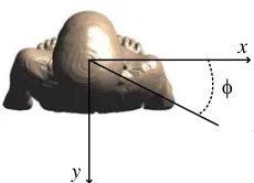
We assume that the data are part of a realization of an intrinsic random function with a variogram γ. The variogram represents the degree of spatial dependence of a spatial stochastic process. In kriging methods, the variogram is experimentally calculated and, then, in order to make estimation, a model of variogram must be set up. In the literature some variogram models exist [20]. Before calculating the experimental variogram, a discussion must be done on the variogram coordinates. SAR values depend on spherical angles of incidence indicated at Figures 1 and 2. These angles of incidence are the angles
θ
z
y
Figure 1. Elevation angle in relation with
Roberta’s body seen from the left.
φ
x
y
Figure 2. Azimuth angle in relation with
of arrival of the MPCs. The kriging method says that the variogram depends on the distance between data points. Since the data points are spherical angles, the variogram coordinates can be defined in two ways: the shortest distance on a sphere or the segment on a projected sphere (also known as geodesic distance and loxodrome). The use of the geodesic distance leads to a problem, when elevation angle is θ = 0◦ or 180◦, SAR values for all φ are located at the same point. Since φ angle modifies the polarization for θ = 0◦ or 180◦, it is better to choose the variogram coordinates as the segment on a projected sphere. The coordinates of variogram are then the angular distance in azimuth and elevation directions, we consider a projected sphere. The experimental variogram is
γexp(Δθ,Δφ) =
1 2N(Δθ,Δφ)
N(Δθ,Δφ)
i,j
(nSAR(θi, φi)−nSAR(θj, φj))2 (5)
with Δφ=φj−φi, Δθ=θj−θi andN(Δθ, Δφ) is the number of pairs ofnSAR spaced by (Δθ,Δφ).
The experimental variogram is obtained by calculating the dissimilarities between the different nSAR
values. For each distance, defined by (Δθ,Δφ), the mean is calculated. However, the experimental variogram cannot be used to assess estimation. A model must be used, the modelization is described in a later section.
By minimizing the estimation variance with the constraint on the weights, we obtain the ordinary kriging system
ΓΛ = Γ0 (6)
with
Γ = ⎛ ⎜ ⎜ ⎝
γ(θ1−θ1, φ1−φ1) . . . γ(θ1−θNs, φ1−φNs) 1
..
. . .. ... ...
γ(θNs−θ1, φNs−φ1) . . . γ(θNs−θNs, φNs −φNs) 1
1 . . . 1 0
⎞ ⎟ ⎟ ⎠
and
Λ = ⎛ ⎜ ⎜ ⎝
λ1
.. .
λNs
μ ⎞ ⎟ ⎟ ⎠
and
Γ0=
⎛ ⎜ ⎜ ⎝
γ(θ1−θ0, φ1−φ0)
.. .
γ(θNs −θ0, φNs−φ0)
1
⎞ ⎟ ⎟ ⎠
whereμ is the Lagrange multiplier. The estimation variance of ordinary kriging is
σ2E =−μ−γ(θ0−θ0, φ0−φ0) + 2
Ns
i=1
λiγ(θi−θ0, φi−φ0) (7)
2.2. Experimental Variogram
The variogram is the key tool of the kriging method. With (5), its estimation can be performed based on numerical nSAR values. We performed FDTD calculations at 2.45 GHz on a child body model, a girl of five years old (Roberta) from the virtual classroom of IT’IS foundation [28]. This body model is made of 66 different kinds of tissues and electrical parameters, permittivity and conductivity are defined thanks to [29].
called horizontal). It represents 684 (= 19×35) different FDTD simulations for each polarization. The source is defined by using the Huygens-Fresnel principle by placing the body model inside a box where the plane wave propagates. Figures 1 and 2 represent the spherical angles of incidence of the plane wave in relation with Roberta’s body position.
The experimental variograms (Figures 3 and 4) have been plotted as a function of (Δθ,Δφ) with Δθ ⊂ [−180◦; 180◦] and Δφ ⊂ [−360◦; 360◦] in order to detect any anistropic behavior. As we can see on Figures 3 and 4, starting from the central point (Δθ = 0◦,Δφ = 0◦), the displacement in any direction is equivalent to a displacement in any displacement in the opposed direction. The point (Δθ= 0◦,Δφ= 0◦) is the reflection point of the experimental variogram.
Thanks to this symmetry, the experimental variogram can be limited to Δθ ⊂ [0; 180◦] and Δφ ⊂ [0; 360◦]. The second observation is the periodicity of the variogram. Usually, the variogram are increasing functions and must present a maximum value. In our case, the variograms reach their maximum values for Δθ = Δφ = 90◦ but decrease further. This periodicity come from spherical symmetry ofSARvalues. The dissimilarity between twonSARvalues at different locations is maximum for a distance of 90◦ between them, in both angular directions. Then, from periodicity in Figures 3 and 4, clearly, we can only take into consideration variograms for 0 ≤ Δθ ≤ 90◦ and 0 ≤ Δφ ≤ 90◦ where are met the first sills. It means that estimation will be possible for a maximum distance of 90◦ in both angular directions and not further.
Figures 5 and 6 present the part of the variograms that will be used in order to find a model. It is important to note that these variograms (5 and 6) show zonal anisotropy: for γexp(Δθ0,Δφ) or
γexp(Δθ,Δφ0) with Δθ0 and Δφ0 taken as constants values, the ranges are always the same but the
sills are different.
-300 -200
-100 0 100
200 300 -100
0 100 x 10-11
Δφ Δθ
γexp
0 0.5 1 1.5
Figure 3. Experimental variogram for θ
-polarization.
-300-200-100 0 100
200 300 -100
0 100 0 0.5 1 1.5 x 10
-11
Δφ Δθ
γexp
Figure 4. Experimental variogram for φ
-polarization.
0 10 20 30 40 50 60 70 80 90
0 0.2 0.4 0.6 0.8 1 1.2
x 10-11
Δθ (°) γ exp
Δφ=0°
Δφ=10°
Δφ=20°
Δφ=30°
Δφ=40°
Δφ=50°
Δφ=60°
Δφ=70°
Δφ=80°
Δφ=90°
Figure 5. Experimental variogram for θ
-polarization.
0 10 20 30 40 50 60 70 80 90
x 10-11
γ exp
Δφ=0°
Δφ=10°
Δφ=20°
Δφ=30°
Δφ=40°
Δφ=50°
Δφ=60°
Δφ=70°
Δφ=80°
Δφ=90°
0 0.5 1 1.5
Δφ (°)
Figure 6. Experimental variogram for φ
2.3. Variogram Model
In the litterature there are few variogram models that are proposed (i.e., conditionnaly negative definite). Outside a fairly limited class of models (linear model with nugget effect) variograms are non-linear in some of their parameters, typically, ranges and anisotropies [21]. For this reason, fitting a variogram model cannot be done entirely automatically. Statistician uses both fitting algorithm and visual similarity between experimental variogram and model of variogram.
Among typical models of variograms, the most appropriate model was found to be the gaussian one:
γgauss(h) =C
1−e−(ha)2
(8)
with h the distance, C the sill and a the range. The literature provides solution for two dimensions variograms that ensure that the variogram is allowed [30].
γ(Δθ,Δφ) =γ1(Δθ) +γ2(Δφ) +γ3(
Δθ2+ Δφ2) (9)
Based on the Levenberg-Marquardt algorithm [31] the parameters ofγ1,γ2andγ3 have been determined
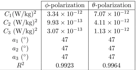
(Table 1) with the R2 in order to evaluate the quality of the fit.
Table 1. Parameters of variogram models for Roberta.
φ-polarization θ-polarization C1(W/kg)2 3.34×10⁻¹² 7.07×10⁻¹²
C2 (W/kg)2 9.93×10⁻¹³ 4.11×10⁻¹²
C3 (W/kg)2 3.07×10⁻¹³ 1.13×10⁻¹²
a1 (◦) 47 47
a2 (◦) 47 47
a3 (◦) 47 47
R2 0.9923 0.9964
3. ESTIMATION
3.1. Estimation on Roberta’s Results
Estimation has been done on Roberta’s nSARvalues by changing the total number of numericalnSAR
values taken into account in the estimation, and changing the number of samples (also called neighbors), Ns, taken into account in (6) to compute each estimation. The total number ofnSARvalues used during
estimation and Ns were adjusted until we found the best configuration that respect two constraints:
to estimate nSAR using a minimum of nSAR values with a limited mean relative error (< 5%) between estimated values and sampled values. We will use the minimum number of values from the 684
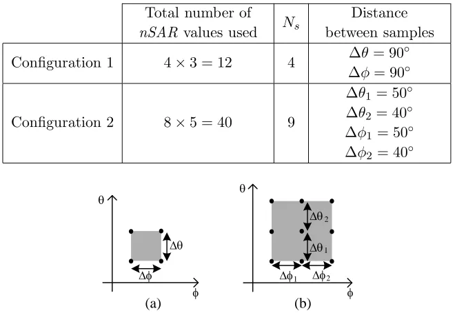
nSAR FDTD values in order to achieve estimation. In order to reach this goal we tested two different configurations described in Table 2.
First, we introduce the two different kinds of neighborhood. At Figure 7(b), Ns is equal to four
and the samples are the black points. These four neighbors are used in order to estimatenSAR values in the grey area. On the left,Ns is equal to nine, these nine samples are used in order to estimatenSAR
values in the grey area.
On Figure 8, configurations 1 and 2 are represented. The black circles represent the locations of
Table 2. Configurations of estimation scenarios.
Total number of
nSAR values used Ns
Distance between samples
Configuration 1 4×3 = 12 4 Δθ= 90
◦
Δφ= 90◦
Configuration 2 8×5 = 40 9
Δθ1 = 50◦
Δθ2 = 40◦
Δφ1 = 50◦
Δφ2 = 40◦
Δφ Δθ
φ θ
Δθ
Δθ
Δφ Δφ φ θ
1 2
1 2
(a) (b)
Figure 7. (a) The four samples neighborhood and (b) the nine samples neighborhood.
0 50 100 150 200 250 300 350 0 50 100 150 200 250 300 350
(a) (b)
0 20 40 60 80 100 120 140 160 180
θ
(°)
0 20 40 60 80 100 120 140 160 180
θ
(°)
φ (°) φ (°)
Figure 8. (a) Configuration 1 and (b) configuration 2.
3.1.1. Tuning the Confidence Interval
The estimation standard deviation can be used in order to introduce the confidence interval [27], at a location of estimation,
[nSAR−νσE,nSAR+νσE] (10)
The ν parameters can be determined by calculating the kriging error | nSAR −nSAR | for each estimation point where we have the value from FDTD calculation and to calculate the probability that the kriging error is greater thanνσE by tuning ν.
Since different configurations lead to different scales of distances between numerical values and estimated values, we choose to calculate the ν parameter on configuration 1 because it is the configuration that leads to the greatest kriging variance and has the most important number of kriging error to calculate. Theν parameter is found by calculating the probability that the distance between estimated values and numerical values are larger than νσE. This probability is equal to the ratio of
the number of kriging error that are bigger thanνσE over the total number of kriging errors [20]. We
search for ν that provides 95% confidence interval.
We foundν= 0.85 to be an appropriate value because: for φ-polarization
and for θ-polarization
Pr (|nSAR−nSAR|≥0.85σE)0.0410 (12)
It provides respectively 95.31% confidence interval forφ-polarization and 95.90% forθ-polarization. The confidence interval is then
[nSAR−0.85σE,nSAR+ 0.85σE] (13)
3.1.2. θ-polarization
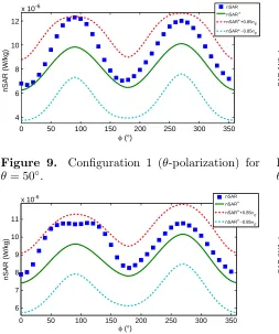
Since estimation cannot be plotted for all spherical angles, estimation plots are shown at θ = 50◦ for configuration 1 and atθ= 20◦ for configuration 2 in function ofφ. Configuration 1 consists in using the minimum number of nSAR values used to perform estimation. At Figure 9 there are a relatively large gaps between estimated values and sampled values. It is due to the fact that, atθ= 50◦, the sampled values are far away. However, the estimated and sampled values are both in the confidence interval.
Previous configuration enables us to minimize the total number of nSAR values used to perform estimation. The next configuration will consist in adding some samples, i.e., nSAR values, in order to decrease the gap between nSAR and nSAR.
Figure 10 represents results for configuration 2. As expected, the estimation is better because the distances between estimated values and numerical values are reduced. More generally, the level of estimation variances decreases because of the new configuration.
3.1.3. φ-polarization
Figures 11 and 12 represent the estimation results on Roberta forφ-polarized incident plane wave. In the point of view of the estimation for the different configurations, we obtain same kind of results as previously.
0 50 100 150 200 250 300 350
x 10-6 nSAR
nSAR * nSAR +0.85σ*
E
nSAR −0.85σ* E
4 6 8 10 12
nSAR (W/kg)
φ (°)
Figure 9. Configuration 1 (θ-polarization) for
θ= 50◦.
0 50 100 150 200 250 300 350
x 10-6
φ (°)
nSAR (W/kg)
nSAR
nSAR*
* E
* E
nSAR +0.85σ
nSAR −0.85σ
4.5 5 5.5 6 6.5 7 7.5 8
Figure 10. Configuration 2 (θ-polarization) for
θ= 20◦.
0 50 100 150 200 250 300 350
x 10-6
φ (°)
nSAR (W/kg)
*
*
E
*
E
nSAR nSAR nSAR +0.85σ nSAR −0.85σ
6 7 8 9 10 11
Figure 11. Configuration 1 (φ-polarization) for
θ= 50◦.
0 50 100 150 200 250 300 350
x 10-6
*
* E
*
E
φ (°)
nSAR nSAR nSAR +0.85σ nSAR −0.85σ
6 6.5 7 7.5 8 8.5
nSAR (W/kg)
Figure 12. Configuration 2 (φ-polarization) for
3.1.4. Results Analysis
All the results that were obtained on Roberta body model show that the estimated values and sampled values are always located inside the confidence interval defined by the kriging variance. However, it is possible to calculate the maximum relative error and mean relative error for configurations 1 and 2. The maximum relative error is defined by
MaxRE = max
|nSAR−nSAR|
nSAR ×100
(14)
And mean relative error is defined by
MeanRE =
|nSAR−nSAR|
nSAR
×100 (15)
Values are given in Table 3 and represent MaxRE and MeanRE over all numerical values. MeanRE for configuration 1 are 8.74% for φ-polarization and 10.7% for θ-polarization. These levels indicate that the error on estimated values are too large when using only 12 nSAR values. Another evidence is the level of MaxRE for configuration 1 (22.6% for φ-polarization and 30.7% for θ-polarization), at some location, the error reaches unacceptable level. The results of configuration 1 show that it is important to include more nSAR values to lead estimation. For configuration 2, MeanRE decreases compared to configuration 1. MeanRE is 2.52% for φ-polarization and 2.57% forθ-polarization which are small level of error. The MaxRE levels are below 15% which is far from the results obtained in configuration 1. By implementing configuration 2, we deeply improved the quality of estimation.
4. VALIDATION ON THELONIOUS RESULTS
The interest of the study on Roberta’s body model was to found the variogram model in order to be able to use the kriging method on any body model by doing the minimum number of simulations. Thanks to Roberta’s FDTD calculations we determine the variogram model (9) and we detected zonal anisotropy (a1 =a2=a3 = 47◦). The interest is then to use the same variogram model on another body model by
testing both configurations.
The sillsC1,C2 andC3 correspond to the variogram reached maximum values at (Δθ= 90◦,Δφ=
0◦), (Δθ= 0◦,Δφ= 90◦) and (Δθ = 90◦,Δφ= 90◦). These values can then be determined thanks to
Table 3. Maximum relative error and mean relative over estimation results.
Configurations Polarization MaxRE MeanRE
1 φ 22.6% 8.74%
θ 30.7% 10.7%
2 φ 14.1% 2.52%
θ 11.3% 2.57%
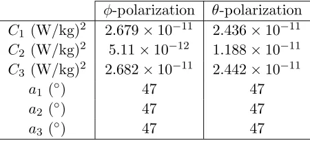
Table 4. Parameters of variogram models for Thelonious.
φ-polarization θ-polarization C1 (W/kg)2 2.679×10⁻¹¹ 2.436×10⁻¹¹
C2 (W/kg)2 5.11×10⁻¹² 1.188×10⁻¹¹
C3 (W/kg)2 2.682×10⁻¹¹ 2.442×10⁻¹¹
a1 (◦) 47 47
a2 (◦) 47 47
only 12 FDTD values located at (θe, φe) withθe= 0◦,90◦and 180◦φe= 0◦,90◦, 180◦and 270◦. Table 4
presents the parameters of Thelonious variogram model for both polarizations. Results of estimation are represented at Figures 13 and 16. Table 5 presents MaxRE and MeanRE for the different configurations over all numerical values.
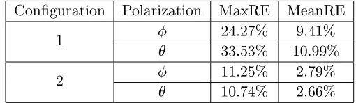
Figures 13 and 14 represent results of estimation of SAR in function of φ for θ = 50◦ in the framework of configuration 1 for both polarization. It can be seen that there is a relatively large gap between estimated values and values calculated by FDTD simulations. At Table 5, mean relative error is under 11% for both polarization but maximum relative error is over 33% for θ-polarization which is quite large.
Figures 15 and 16 represent results of estimation of SAR in function of φ for θ = 20◦ in the framework of configuration 2 for both polarization. Switching from four neighbors to nine neighbors (i.e., addingnSAR values calculated by FDTD simulations) improves greatly the quality of estimation because estimated values are really close to values calculated by FDTD simulations. At Table 5, mean relative errors are under 3% and maximum relative error are under 12%.
0 50 100 150 200 250 300 350
x 10-6
nSAR (W/kg) * * E * E φ (°) nSAR nSAR nSAR +0.85σ
nSAR −0.85σ 2 4 6 8 10 12 14 16
Figure 13. Configuration 1 (θ-polarization) for θ= 50◦ on Thelonious.
0 50 100 150 200 250 300 350
x 10-6
nSAR (W/kg) * * E * E φ (°) nSAR nSAR nSAR +0.85σ
nSAR −0.85σ 2 4 6 8 10 12 14 16
Figure 14. Configuration 1 (φ-polarization) for θ= 50◦ on Thelonious.
0 50 100 150 200 250 300 350
x 10-6
nSAR (W/kg) * * E * E φ (°) nSAR nSAR nSAR +0.85σ
nSAR −0.85σ
2 4 6 8 10
Figure 15. Configuration 2 (θ-polarization) for θ= 20◦ on Thelonious.
0 50 100 150 200 250 300 350
x 10-6
* * E * E φ (°) nSAR nSAR nSAR +0.85σ
nSAR −0.85σ
4 6 8 10 12 nSAR (W/kg)
Figure 16. Configuration 2 (φ-polarization) for θ= 20◦ on Thelonious.
Table 5. Maximum relative error and mean relative over estimation results of Thelonious.
Configuration Polarization MaxRE MeanRE
1 φ 24.27% 9.41%
θ 33.53% 10.99%
2 φ 11.25% 2.79%
5. CONCLUSION
For the first time, a statistical analysis of exposure leads to the development of an expression of expectation of SAR and its standard deviation over the complex random amplitude that is due to the electromagnetic environment. It has been noticed that these equations are expressed in functions of whole body Specific Absorption Rate values that are due to a simple plane wave exposure.
An estimation method is necessary in order to calculate allnSAR for each angle of incidence. The kriging method that has proven its efficiency in many domains has been applied to our results on two different children body models. By using the kriging method we demonstrate its efficiency by radically reducing the number of samples used to lead the estimation. First, we used the 684 nSAR values that come from FDTD simulations to calculate the experimental variogram. A model of variogram has been fitted on the experimental variogram. The estimation on configuration 1 uses only 12nSARvalues that come from FDTD simulations. The results of estimation and its analysis have shown that there were a relatively large gap between estimatednSARvalues andnSARvalues calculated by FDTD simulations. Configuration 1 leads to 30% of mean relative error at some location which is an unacceptable amount of error in our study. The reason is that our final goal is to do a sensitivity analysis of SAR and σSAR2 to the wireless channel parameters. Since, these analytical expressions SAR and σSAR2 depend onnSARvalues estimated by kriging method, then, estimatednSARvalues must be accurate otherwise the sensitivity analysis would be wrong. This is the reason why configuration 1 must be improved. Configuration 1 has been modified by adding some new samples in order to reduce the mean relative error and maximum relative error. Configuration 2 consists in estimating nSAR values thanks to 40 nSAR values that come from FDTD simulations. Analysis of results on configuration 2 shows that we radically reduced the errors (Mean relative error under 3% and Maximum relative error under 15%). It shows that the best configuration to estimate rapidly nSAR and with the minimum error is the configuration 2 using only 40nSAR values.
REFERENCES
1. ICNIRP, “Guidelines for limiting exposure to time-varying electric, magnetic, and electromagnetic fields (up to 300 GHz),” Health Physics, Vol. 75, No. 4, 442, 1998.
2. ICNIRP, “Statement on the guidelines for limiting exposure to time-varying electric, magnetic, and electromagnetic fields (up to 300 GHz),”Health Physics, Vol. 97, No. 3, 257–258, Sep. 2009. 3. ICNIRP, “Exposure to high frequency electromagnetic fields, biological effiects and health
consequences (100 kHz–300 GHz),” Review of the Scientific Evidence and Health Consequences, ICNIRP 16, 2009.
4. Habachi, A. E., E. Conil, A. Hadjem, E. Vazquez, M. F. Wong, A. Gati, G. Fleury, and J. Wiart, “Statistical analysis of whole-body absorption depending on anatomical human characteristics at a frequency of 2.1 GHz,” Phys. Med. Biol., Vol. 55, 1875–1887, 2010.
5. Dimbylow, P. J., A. Hirata, and T. Nagaoka, “Inter-comparison of whole-body averaged SAR in European and Japanese voxel phantoms,”Phys. Med. Biol., Vol. 53, 5883–5897, 2008.
6. Findlay, R. P. and P. J. Dimbylow, “Effects of posture on FDTD calculations of specific absorption rate in a voxel model of the human body,”Phys. Med. Biol., Vol. 50, 3825–3835, 2005.
7. Akimoto, S., T. Nagaoka, K. Saito, S. Watanabe, M. Takahashi, and K. Ito, “Comparison of SAR in realistic fetus models of two fetal positions exposed to electromagnetic wave from business portable radio close to maternal abdomen,”EMBC Annual International Conference of the IEEE, 734–737, Buenos Aires, 2010.
8. Quitin, F., “Channel modeling for polarized MIMO systems,” Ph.D. Thesis, Universit´e Libre de Bruxelles, 2011.
11. K¨uhn, S., W. Jennings, A. Christ, and N. Kuster, “Assessment of induced radio-frequency electromagnetic fields in various anatomical human body models,”Phys. Med. Biol., Vol. 54, 875– 890, 2009.
12. Vermeeren, G., G. Joseph, C. Olivier, and F. Martens, “Statistical multipath exposure of a human in a realistic electromagnetic environment,” Health Physics, Vol. 94, 345–354, 2008.
13. Kientega, T., E. Conil, A. Hadjem, E. Richalot, A. Gati, M. F. Wong, O. Picon, and J. Wiart, “A surrogate model to assess the whole-body sar induced by multiple plane waves at 2.4 GHz,” Ann. Telecommun., Vol. 66, 419–428, 2011.
14. Vermeeren, G., W. Joseph, and L. Martens, “Statistical multi-path exposure method for assessing the whole-body SAR in a heterogeneous human body model in a realistic environment,”
Bioelectromagnetics, Vol. 34, 240–251, 2013.
15. Thielens, A., G. Vermeeren, W. Joseph, and L. Martens, “Stochastic method for determination of the organ-specific averaged SAR in realistic environments at 950 MHz,” Bioelectromagnetics, Vol. 34, 549–562, 2013.
16. Bamba, A., W. Joseph, G. Vermeeren, E. Tanghe, D. P. Gaillot, J. Andersen, J. Nielsen, M. Lienard, and L. Martens, “Validation of experimental whole-body SAR assessment method in a complex indoor environment,”Bioelectromagnetics, Vol. 34, 122–132, 2013.
17. Bernardi, P., M. Cavagnaro, S. Pisa, and E. Piuzzi, “Human exposure to radio base-station antennas in urban environment,”IEEE Transactions on Microwave Theory and Techniques, Vol. 48, No. 11, 1996–2002, 2000.
18. Silly-Carette, J., D. Lautru, M. F. Wong, A. Gati, J. Wiart, and V. Fouad. Hanna, “Variability on the propagation of a plane wave using stochastic collocation methods in a bioelectromagnetic application,”IEEE Microwave Communications Letters, Vol. 19, No. 4, 185–187, 2009.
19. Ghanmi, A., N. Varsier, A. Hadjem, J. Wiart, C. Person, O. Picon, and E. Conil, “Exposure analysis of children reproductive organs to EMF emitted by a mobile phone placed nearby,”BioEM 2013: Joint Meeting of the Bioelectromagnetics Society (BEMS) and the European BioElectromagnetics Association (EBEA), 2013.
20. Wackernagel, H.,Multivariate Geostatistics, Springer, 1998. 21. Cressie, N., Statistics for Spatial Data, Wiley-Interscience, 1992.
22. Yee, K. S., “Numerical solution of initial boundary value problems involving maxwells equations in isotropic media,”IEEE Trans. on Antennas and Propagation, Vol. 14, No. 3, 302–307, 1966. 23. Taflove, A. and S. Hagness, Computational Electrodynamics: The Finite-DIfference Time-domain
method, 3rd Edition, Artech House, 2005.
24. Quitin, F., C. Oestges, F. Horlin, and P. De Doncker, “Channel correlation and cross-polar ratio in multi-polarized MIMO channels: Analytical derivation and experimental validation,” IEEE 68th Vehicular Technology Conference, VTC 2008-Fall, 1–5, 2008.
25. Sibille, A., C. Oestges, and A. Zanella, MIMO from Theory to Implementation, Elsevier, 2010. 26. IEEE Computer Society, “Part 11: Wireless LAN medium access control (MAC) and physical layer
(PHY) specifications,” IEEE Standard Association, Mar. 2012.
27. Chiles, J. P. and P. Delfiner,Geostatistics: Modeling Spatial Uncertainty,Wiley-Interscience, 1990. 28. Christ, A., et al., “The virtual family-development of surface-based anatomical models of two adults
and two children for dosimetric simulations,” Phys. Med. Biol., Vol. 55, 23–38, 2010.
29. Gabriel, S., R. W. Lau, and C. Gabriel, “The dielectric properties of biological tissues: III. Parametric models for the dielectric spectrum of tissues,” Phys. Med. Biol., Vol. 41, 2271–2293, 1996.
30. Myers, D. E. and A. Journel, “Variograms with zonal anisotropies non-invertible kriging systems,”
Mathematical Geology, Vol. 7, 779–785, 1990.
31. Gill, P. E. and W. Murray, “Algorithms for the solution of the nonlinear least-squares problem,”