Optimizing the usage of 2D and 3D transformations to improve the BM3D image denoising algorithm

(1)

Western University Western University

Scholarship@Western

Electronic Thesis and Dissertation Repository

8-26-2019 11:30 AM

Optimizing the usage of 2D and 3D transformations to improve

the BM3D image denoising algorithm

Zaied Zaman

The University of Western Ontario

Supervisor

El-Sakka, Mahmoud

The University of Western Ontario Graduate Program in Computer Science

A thesis submitted in partial fulfillment of the requirements for the degree in Master of Science © Zaied Zaman 2019

Follow this and additional works at: https://ir.lib.uwo.ca/etd

Recommended Citation Recommended Citation

Zaman, Zaied, "Optimizing the usage of 2D and 3D transformations to improve the BM3D image denoising algorithm" (2019). Electronic Thesis and Dissertation Repository. 6523.

https://ir.lib.uwo.ca/etd/6523

This Dissertation/Thesis is brought to you for free and open access by Scholarship@Western. It has been accepted for inclusion in Electronic Thesis and Dissertation Repository by an authorized administrator of

(2)

Image denoising is one of the most important preprocessing steps before a wide range of

applications such as image restoration, visual tracking, image segmentation, etc. Numerous

studies have been conducted to improve the denoising performance. Block Matching and 3D

(BM3D) filteringis the current state-of-the-art algorithm in image denoising and can provide

better denoising performance than other existing methods. However, still, there is scope to

im-prove the performance of BM3D. In this thesis, we have pointed out an aspect of the algorithm which can be improved and suggested an approach to improve it. We have proposed to perform

a 2D and 3D transformation on certain patches rather than performing a 3D transformation on

all the patches.

(3)

Lay Summary

Pixel values of natural images get corrupted by noise mostly in transmission and

acquisi-tion steps. It is needed to denoise or estimate the true pixel values from noisy pixel values

for sophisticated imaging applications. Block-Matching and 3D filtering (BM3D) algorithm

is one of the state-of-the-art algorithms to denoise natural images. In this thesis, we aim at

improving the denoising performance of BM3D even further. BM3D uses a fixed approach

(3D transformation) for the whole image. In this thesis, we have proposed an adaptive way to choose between two techniques (2D transformation and 3D transformation) for appropriate

scenarios.

(4)

I would like to express my heartiest gratitude to the Almighty for the strength, patience,

in-telligence and endless kindness he provided me with to finalize this thesis. I am grateful to

my honorable supervisor Dr. Mahmoud R. El-Sakka for his valuable direction, guidance,

com-ments, and encouragement throughout this work. It was an absolute honor and privilege to

work with such a modest and wise person like him. His wisdom and notable thoughts have

helped this thesis become an ultimate success. He redirected my view of thinking to a progres-sive path every time I discussed my research problems with him. This dissertation under his

supervision will always be a remarkable experience in my life. I would like to acknowledge

my heartiest gratitude to all the professors of The University of Western Ontario who helped

me through many courses to build my background for this dissertation. I acknowledge the

sup-port of my friends, family members and research group members throughout this long tiring

period. Finally, I would like to thank The Department of Computer Science at The University

of Western Ontario to fund my graduate study.

(5)

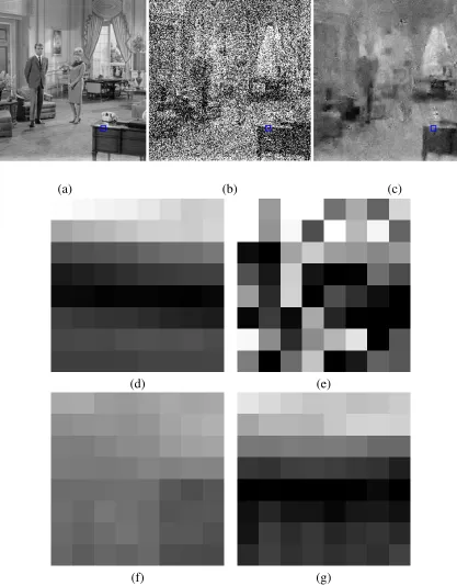
3.2 (a) Original image (b) Noisy image corrupted by gaussian noise of level 100 (c) Denoised image produced by BM3D (d) Original patch located at row 201 and column 185 (e) Noisy patch (f) the patch after 3D transform (g) the patch after 2D transform; we have marked the patch by blue square in the corresponding images . . . 45

3.3 (a) Original image (b) Noisy image corrupted by gaussian noise of level 100 (c) Denoised image produced by BM3D (d) Original patch located at row 209 and column 41(e) Noisy patch (f) the patch after 3D transform (g) the patch after 2D transform; we have marked the patch by blue square in corresponding images . . . 46

3.4 (a) Original image (b) Noisy image corrupted by gaussian noise of level 60 (c) Denoised image produced by BM3D (d) Original patch located at row 9 and column 225 (e) Noisy patch (f) the patch after 3D transform (g) the patch after 2D transform; we have marked the patch by blue square in corresponding images 47 3.5 (a) Original image (b) Noisy image corrupted by gaussian noise of level 100 (c) Denoised image produced by BM3D (d) Original patch located at row 249 and column 249 (e) Noisy patch (f) the patch after 3D transform (g) the patch after 2D transform; we have marked the patch by blue square in corresponding images . . . 48

4.1 Test Images: (a) Lena (b) Boats (c) Goldhill (d) Man (e) Barbara (f) Peppers (g) Couple (h) Baboon . . . 50

4.2 Visual result ((a) the original image, (b) the noisy image corrupted by gaussian noise of noise level 30, (c) the denoised image produced by BM3D and (d) the denoised image produced by our experimented method case 2: Applying 2D processing having the number of similar patches less than or equal to four) . . . 59

4.3 Visual result with zoom-in ((a) the original image, (b) the noisy image cor-rupted by gaussian noise of noise level 30, (c) the denoised image produced by BM3D and (d) the denoised image produced by our experimented method case 2: Applying 2D processing having the number of similar patches less than or equal to four) . . . 60

(10)

denoised image produced by our experimented method case 1: Applying 2D

processing having the number of similar patches less than or equal to two) . . . 61

4.5 Visual result with zoom-in ((a) the original image, (b) the noisy image

cor-rupted by gaussian noise of noise level 20, (c) the denoised image produced by

BM3D and (d) the denoised image produced by our experimented method case

1: Applying 2D processing having the number of similar patches less than or

equal to two) . . . 62

4.6 Visual result ((a) the original image, (b) the noisy image corrupted by gaussian noise of noise level 10, (c) the denoised image produced by BM3D and (d) the

processing having the number of similar patches less than or equal to four) . . . 63

2: Applying 2D processing having the number of similar patches less than or equal to four) . . . 64

4.8 Visual result ((a) the original image, (b) the noisy image corrupted by gaussian

noise of noise level 10, (c) the denoised image produced by BM3D and (d) the

cor-rupted by gaussian noise of noise level 10, (c) the denoised image produced by BM3D and (d) the denoised image produced by our experimented method case

(11)

processing having the number of similar patches less than or equal to four) . . . 69 4.13 Visual result with zoom-in ((a) the original image, (b) the noisy image

equal to four) . . . 70

processing having the number of similar patches less than or equal to two) . . . 71 4.15 Visual result with zoom-in ((a) the original image, (b) the noisy image

processing having the number of similar patches less than or equal to four) . . . 73 4.17 Visual result with zoom-in ((a) the original image, (b) the noisy image

equal to four) . . . 74

(12)

4.1 Comparison of PSNR of BM3D and Experimented Method Case 1: Applying

2D processing when having number of similar patches less than or equal to

two. Exp: The PSNR of the denoised image produced by our experimented

method, Imp: PSNR difference between the denoised images produced by our

experimented method and the BM3D method in dB . . . 52

4.2 Comparison of PSNR of BM3D and Experimented Method Case 2 : Applying 2D processing when having number of similar patches less than or equal to

four. Exp: The PSNR of the denoised image produced by our experimented

method, Imp: The PSNR difference between the denoised images produced by

our experimented method and the BM3D method in dB . . . 53

4.3 Comparison of average PSNR(dB) of BM3D, Experimented Method case 1:

(Applying 2D processing when having number of similar patches less than or

equal to two), Experimented Method Case 2: (Applying 2D processing when

having number of similar patches less than or equal to four) . . . 54

4.4 Comparison of runtime (seconds) of BM3D and Experimented Method case 1: Applying 2D processing when having number of similar patches less than or

equal to two, Exp: The runtime(seconds) of the denoised image produced by

our experimented method case 1, Imp: runtime (seconds) difference between

the denoised images produced by our experimented method and the BM3D

method . . . 55

4.5 Comparison of runtime (seconds) of BM3D and Experimented Method case 2:

Applying 2D processing when having number of similar patches less than or

equal to four, Exp: The runtime(seconds) of the denoised image produced by

our experimented method case 2, Imp: runtime (seconds) difference between the denoised images produced by our experimented method and the BM3D

method . . . 56

4.6 Percentage of patches having two similar patches . . . 57

4.7 Percentage of patches having two or four similar patches . . . 57

(13)

Chapter 1 Introduction

A digital image can be defined as two-dimensional discrete functions which can be represented

by a two-dimensional matrix. The height of the image is the number of rows of the matrix

and the width of the image is the number of columns of the matrix. Each of the entries in this

matrix is defined as a pixel. If we represent this matrix as f, then f(i, j) represents a specific

pixel which is located at spatial coordinate (i, j). The value of f(i, j) is called a pixel value,

intensity value, brightness value interchangeably.

During the acquisition or transmission, digital images may be contaminated by noise.

Faulty instruments, interfering natural phenomena, lossy compression can be accounted for

as some of the many reasons for contaminations. True pixel values of the image get distorted because of noise. This distorted pixel values can produce erroneous results in sophisticated

imaging applications such as satellite imaging, medical imaging, etc. So, the denoising is

needed to estimate the true pixel value before the image goes to these applications. Thus,

Image denoising performance is of high importance and considered as the most important

pre-processing step before these sophisticated applications.

Image denoising is well studied over the past decades. Among other approaches, Block

Matching and 3D(BM3D) filtering is an algorithm developed to improve the denoising

perfor-mance. BM3D is currently the state-of-the-art algorithm for image denoising.

In this chapter, we will discuss our problem description and will point out the objectives of this thesis. We will also describe the major contributions and outline of this thesis.

1.1 Motivations

Digital noise can be of many types. Different techniques are available to denoise different

types of noises in the literature. Noise is random. According to the central limit theorem [28],

irrespective of the base distribution, if we sum samples taken from a random distribution, the

(14)

distribution approaches to normal or Gaussian distribution. As we are simulating practical

scenarios, where the source of noise is seldom known, if we assume that the noise affecting our

image is Gaussian, we can have a better scenario.

During the years, various approaches have been developed to denoise gaussian noisy

im-ages. BM3D is the current state-of-the-art algorithm to denoise gaussian noisy imim-ages. BM3D

utilizes the redundancy of similar patches available in the image. BM3D works in two steps. It

produces a basic estimate image in the first step. Then, it uses Wiener filtering to compute the

final denoised image. The basic estimate image is to better facilitate the Wiener filtering.

It is worth mentioning that the performance of BM3D degrades for higher noise levels.

Hence, the performance is still not sufficient for sensitive applications.

1.2 Problem Statement

To exploit the existing correlation between patches in the natural images, BM3D performs 3D transform regardless of whether enough similar patches are available or not. If enough similar

patches are not available, exploiting the correlation between dissimilar patches might produce

degraded denoised estimation. Hence, we suggest exploiting only the correlation between the

patch itself to get a better-denoised estimate if enough similar patches are not available. We

can exploit the correlation between the patch itself by performing a 2D transform when enough

similar patches are not available.

1.3 Our Objective

Our objective is to improve the denoising performance of BM3D. BM3D uses 3D

transforma-tion irrespective of whether enough similar patches are available or not. We aim at finding an

optimized way of utilizing both 2D and 3D transformation.

1.4 Thesis Contribution

The major contribution of this thesis is the improvement of the performance of the BM3D

algorithm. We will show that if we attempt to combine dissimilar patches to perform 3D

trans-form to exploit the correlation between patches, we might end up with a degraded denoising

performance. We will also show that if enough number of similar patches are not available in

the image, it is better to perform a 2D transform to produce a denoised version with the help of

(15)

1.5. ThesisOutline 3

1.5 Thesis Outline

In Chapter 2, we will discuss the image denoising in details. We will introduce different types of noise, their effects on the images, our reason to consider a specific type, the different

techniques available to denoise this specific type of noise, details of BM3D and improvements

of BM3D in recent years.

In Chapter 3, we will discuss our approach to improve the performance of BM3D in de-tails.

InChapter 4, we will present the experimental results produced by our suggested approach and also compare these results with the results produced by BM3D.

(16)

Background Studies

Random variation of image intensities can be defined as a noise in digital images. An image

can be corrupted by noise in its acquisition and transmission. Mostly, the values acquired

by image sensors are contaminated by noise because of imperfect instruments, problems with

the data acquisition process and interfering natural phenomenas[30][2]. Figure 2.1 shows an

example of a noisy image. The left image is the original image and the right image is the noisy

image corrupted by Gaussian noise of standard deviation,σ=20.

Figure 2.1: Example of a noisy image

2.1 Image Noise

The noises which contaminate the image are random. Figure 2.2 will help us to understand the

effect of noise on the true pixel value. We have plotted the pixel values of a specific row of

both of the image from Figure 2.1. The left image is the plot of pixel values of row=10 from

the original image and the right image is the plot of the same row from the noisy image. We

(17)

2.2. NoiseTypes 5

can observe that the pixel values were almost uniform when they were not corrupted by noise.

When these pixel values are corrupted by Gaussian noise they took the shape of a Gaussian

distribution.

In order to denoise, we need to approximate the noise mathematically. In order to approximate the noise, we choose different noise models for different noise cases.

Figure 2.2: Effect of noise on pixel true value

2.2 Noise Types

We will divide the noise between two types based on the correlation of noise values with pixel

values.

1. Spatially independent noise

2. Spatially dependent noise

In the following sections, we will discuss these two types of noise. We will briefly discuss

another special type of noise named Impulse noise.

2.3 Spatially Independent Noises

If the noise is independent of spatial coordinates and has no correlation with pixel true value,

(18)

The following equation represents the spatially independent noise model,

z(i, j)= y(i, j)+η(i, j) (2.1)

Here, i and j represents the pixel coordinates. y(i, j) is the true pixel intensity. η(i, j) is the

spatially independent noise.z(i, j) is the noisy image.

There are many types of spatially independent noises and we will discuss a few of them in the following sections.

2.4 Gaussian Noise

The Gaussian noise follows the Gaussian distribution. The "Amplifier Noise" is a major part of

the "read noise" of an image sensor. Read noise is the amount of noise generated by electronics

as the charge present in the pixels is transferred to the camera. This "Amplifier Noise" is

modeled as Gaussian Noise.

Gaussian Noise is mostly used as a noise model for denoising because it is mathematically

convenient.

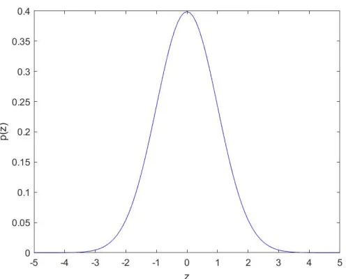
The Probability Density Function (pdf) of Gaussian distibution [20] is as follows,

p(z)= √ 1

2πσ2e

−(z−µ)2

2σ2 _(2.2)

Here,µis mean andσis the standard deviation of the distribution.

(19)

2.5. RayleighNoise 7

Figure 2.3: Gaussian Distribution pdf

The Normal distribution is a special case of Gaussian distribution where the mean is 0 and the standard deviation is 1. In Gaussian distribution, around 68% values will be within one

standard deviation from the mean.

Figure 2.4 shows an example of a noisy image corrupted by Gaussian noise with mean 0 and standard deviation 10.

Figure 2.4: Example of Gaussian noisy image

2.5 Rayleigh Noise

Rayleigh Noise follows Rayleigh distribution. Signal values are almost zero in the background

(20)

Figure 2.5: Rayleigh distribution pdf

Figure 2.6: Effect ofbon Rayleigh distribution

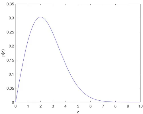
noise. The Pdf equation of the Rayleigh distribution is as follows [20],

p(z)=

        

2(z−a)

b e

−(z−a)2

b z≥ a

0 z< a

(2.3)

Here,brepresents the spread of the distribution andarepresents the shift from the origin.

Figure 2.5 shows the pdf of the Rayleigh distribution withb=2 anda=0.

The shape of the Rayleigh distribution is skewed to the right. It can be useful for

approxi-mating skewed histograms.

Figure 2.6 shows the effect of different values ofbon the Rayleigh distribution.

In Figure 2.7, the left image is the actual cameraman image and the right image is the

(21)

2.6. GammaNoise 9

Figure 2.7: Example of Rayleigh noisy image

2.6 Gamma Noise

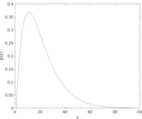
Noises which occur in the laser-based images can be modeled as Gamma noise. The following

is the equation of the pdf of Gamma noise,

p(z)=

        

abz(b−1) (b−1)! e

(−az) _z_≥₀

0 z<0

(2.4)

Here,bis the shape parameter andais the rate parameter.

Figure 2.8 shows the pdf of Gamma distribution withb=2 anda=0.

(22)

Figure 2.9 shows the effect of the parameters on the distribution. The left image is the effect

of variousavalues and the right image is the effect of variousbvalues.

Figure 2.9: Effect of parameters on Gamma distribution

cameraman image corrupted by Gamma noise with parametersa= 5 andb= 5.

Figure 2.10: Example of Gamma noisy image

2.7 Exponential Noise

In Channel-based communication, noises can be modeled as Exponential noise. Actually, the

Exponential distribution is a variant of Gamma distribution whereb= 1.

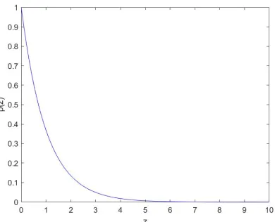
The following is the pdf equation of the Exponential noise[20],

p(z)=

        

ae−az _z_≥₀

0 z<0

(23)

2.8. UniformNoise 11

Here,ais the rate parameter. It represents how quickly the Exponential pdf is decaying.

Figure 2.11 shows the pdf of Exponential distribution witha=1.

Figure 2.11: Exponential distribution pdf

cameraman image corrupted by Exponential noise with parametera=0.1.

Figure 2.12: Example of Exponential noisy image

2.8 Uniform Noise

This noise model does not resemble any practical situation.

The pdf equation of the uniform noise is following[20],

p(z)=

        

1

b−a b≤z≥a

0 otherwise

(24)

Here, all the values between a and b have an equal probability of occurring. The pdf of

uniform noise is following,

Figure 2.13 shows the pdf of Exponential distribution withb=5 anda=2.

Figure 2.13: Uniform Distribution pdf

cameraman image corrupted by uniform noise with parameterb= 40 anda=20.

Figure 2.14: Example of uniform noisy image

2.9 Additive White Gaussian Noise

When the noise has constant power spectral density, it is called as White noise[20]. Power

spectral density shows how much power is contained in each of the spectral components. A

White noise signal is constituted by a series of samples that are independent and generated

(25)

2.10. SpatiallyDependentNoise 13

number generator in which all the samples follow a given Gaussian distribution is called White

Gaussian noise.

2.10 Spatially Dependent Noise

This type of noise gets multiplied with the original signal. Spatially dependent noise has a

correlation with a true pixel value. The spatially dependent noise model is following,

z(i, j)=y(i, j)η(i, j) (2.7)

Here, y(i,j) is the pixel intensity andη(i,j) is the spatially dependent noise at (i, j) coordinate.z(i, j)

is the noisy pixel intensity. In the following section, we will discuss a common spatially

de-pendent noise referred to speckle noise.

2.11 Speckle Noise

In almost all coherent systems, the noises can be modeled as speckle noise. Mainly, the source of this kind of noise is random interference between coherent returns. It follows Gamma

dis-tribution.

cameraman image corrupted by speckle noise.

(26)

2.12 Impulse Noise

The pdf equation of impulse noise is following[20],

p(z)=

                

Pa z= a

Pb z= b

0 otherwise

(2.8)

Figure 2.16 shows the pdf of impulse noise.

Figure 2.16: Impulse noise pdf

Ifb> a, gray-level b will appear as a light dot in the image. Conversely, level a will appear

like a dark dot. If either Pa or Pb is zero, the impulse noise is called unipolar. Otherwise, it

is called bipolar. If neither of them is zero and if they are approximately equal, impulse noise

values will resemble salt-and-pepper granules randomly distributed over the image. For this

reason, bipolar impulse noise is also called salt-and-pepper noise.

Noise impulses can be negative or positive. Impulse noises are very large compared to the

image pixel intensity values, impulse noise is digitized as extreme(pure black or white) values

in the image. Thus the assumption is thataandbis equal to the minimum and maximum values allowed in the digitized image. Negative impulses appear as a black dot and positive impulses

appear as a white dot in the image. For, 8 bit image,a=0(black) andb= 255(white).

In situations where quick transients, such as faulty switching, take place during imaging,

noises can be modeled as impulse noise.

In Figure 2.17, the left image is the actual image and the right image is the image corrupted

(27)

2.13. OurConsideredNoise 15

Figure 2.17: Example of impulse noisy image

2.13 Our Considered Noise

Noises of different types are different in nature. They also have different denoising techniques

for each of them. For the rest of our discussion, we are going to consider the additive White

Gaussian noise and some of the denoising techniques for the natural images which are cor-rupted by this noise. Our considered Noise has following properties,

• Additive: We are considering signal independent noise. Mathematically it will be added

to the original signal or pixel true value.

• Independent and Identically distributed: The noise samples we are considering, are

inde-pendent of each other. All of our considered noise samples will be drawn from the same

distribution.

• Gaussian: According to central limit theorem, irrespective of underlying distribution of

a population (with meanµand standard deviationσ, if we take a number of samples of size N from the population, then the sample mean to follow a normal distribution with a

mean ofµand a standard deviation of σ/√N [28][16][15]. It signifies that irrespective

of base distribution the probability distribution curve will approach Gaussian or normal

distribution. In other words, the sum of independent and identically distributed random

variables(with finite mean and variance) approaches normal distribution as sample size

(28)

2.14 Image Denoising

In the previous section, we have discussed the random noises and how to model them. In this

section, we will discuss various approaches to denoise noisy images.

There are two basic approaches to image denoising. They are following,

1. Spatial filtering methods

2. Transform domain filtering methods

We will discuss them in the following sections.

2.15 Spatial Filtering Methods

In the spatial filtering methods, we aim to denoise the noisy pixel values in the spatial domain.

Spatial filters can be further classified into two following types,

1. Linear spatial filters

2. Non-linear spatial filters

We will discuss them in the following sections.

2.16 Linear Spatial Filters

In linear spatial filtering, the value of an output pixel is a linear combination of neighborhood

values. There are various types of linear spatial filters. Mean filter is the most common one.

We will discuss the mean filter in the following section,

2.17 Arithmetic Mean Filter

The mean filter aims at finding an estimate which minimizes the mean square error between the noisy value and the respective estimate in the spatial domain. Let Sxy represent the set

of coordinates in a rectangular sub-image window size ofm×ncentered at point (x,y). The

Arithmetic Mean filtering process computes the average value of the corrupted image, g(x,y)

in the area defined bySxy. The value of the restored image ˆf at any point (x,y) is simply the

arithmetic mean computed using the pixels in the region defined by Sxy. The equation is as

(29)

2.18. MinimumMeanSquareError(Wiener) Filtering 17

ˆ

f(x,y)= 1 mn

X

(s,t)Sxy

g(s,t) (2.9)

Mean filters actually smooth the local variations in the image. The Denoised image might

be highly blurred.

Figure 2.18 shows an example of a denoised image by the Arithmetic Mean filtering.

(a) Actual Image (b) Noisy Image (c) Denoised Image

Figure 2.18: Example of denoised image by mean filter

2.18 Minimum Mean Square Error(Wiener) Filtering

The objective of this filter is to find an estimate, ˆf of the uncorrupted image f such that the

mean square error between them is minimized. This error measure is given by[20],

e2 = E{(f − fˆ)2} (2.10)

Here, E{.} is the expected value of the argument. Wiener filter is used in the frequency

domain. It is not a spatial filter but a linear filter. Let us assume, we have a noisy image, g(u,v)

and we will denote the Discrete Fourier Transform(DFT) of the image as G(u,v). In the spatial

domain, we usually convolute the filter kernel with the image to get the filtered output. In the

frequency domain, the convolution operation becomes the multiplication operation. So, if we

multiply the DFT of the Wiener filter with the noisy transformed image, we will get the filtered

image. The following is the equation of DFT of the image estimated by Wiener filter[20],

ˆ

F(u,v)= H

∗₍_u,_v₎_S

f(u,v)

Sf(u,v)|H(u,v)|2+Sη(u,v)

G(u,v) (2.11)

Here, H(u,v) is the DFT of the Degradation function or Point Spread Function,H∗(u,v) is

(30)

spectrum of the undegraded image. We will get the denoised image in the spatial domain by

the inverse transform the DFT estimate.

Figure 2.19 shows an example of a Wiener filtered image.

Figure 2.19: Example of Wiener filtered image

2.19 Non-linear Spatial Filter

One of the main problems associated with the linear spatial filters is that they blur the edges. Non-linear Spatial filters give better denoising result with less blurring for some of the noise

models. The Median filter is the most common Non-linear spatial filter. We will discuss the

Median filter in the following section.

2.20 Median Filter

The Median filter is one of the most popular order-statistics filters. Order-statistics filters are

spatial filters whose response is based on ordering the pixels contained in the image area

en-compassed by the filter. The response of the filter at any point is determined by the ranking

result. The Median filter replaces the value of a pixel by the median of the gray levels in the neighborhood of that pixel. We can understand it by the following equation[20],

ˆ

f(x,y)=median

(s,t)Sxy

{g(s,t)} (2.12)

Median filters are particularly effective in the presence of both unipolar and bipolar impulse

(31)

2.21. AdaptiveMedianFilter(ADM) 19

Figure 2.20: Example of Median filtered image

2.21 Adaptive Median Filter(ADM)

The performance of the Median filter discussed in the previous section degrades if the spatial

density of impulse noise is high[20]. The Adaptive Median filter can perform well even if

the density of impulse noise is high. Adaptive Median Filter (AMF) works in a rectangular window area, Sxy. Depending on the gray level values in the area, the algorithm changes the

size of the window area. We will representzminas the minimum gray level value inSxy,zmaxas

the maximum gray level value inSxy,zmed as the median of gray levels inSxy, zxy as the gray

level at coordinates (x,y),Smaxas the maximum allowed size ofSxy.

We will briefly describe the algorithm here. AMF works in two levels, we will denote them as

level A and level B. In level A, the algorithm searches for a region wherezmed is greater than

zminand less than zmax. It keeps increasing search size as long as this condition does not meet.

If the condition is satisfied in any region, the algorithm proceeds to level B. In level B, ifzxy

is more thanzmin and less thanzmaxin that region, then the denoised pixel value at (x,y) iszxy,

otherwise, the denoised value is zmed. If the algorithm could not proceed to level B and the

search area becomes greater thanSxy, then the denoised pixel value at (x,y) iszxy.

Figure 2.21 shows an example of ADM filtered image corrupted by Gaussian noise and

(32)

Figure 2.21: Example of ADM filtered image for Gaussian noisy image

Figure 2.22: Example of ADM filtered image for impulse noisy image

2.22 Transform Domain Filtering Based Methods

In transform domain filtering methods, we will not filter in the spatial domain, rather we will

transform the pixel intensity values into any other transform domain. We will choose transform

domain such that in that domain, we can separate noise and signal values as better as we can.

Then we will perform the filtering on the transformed coefficients so that the separated noise

gets eliminated and we get a sparse representation. Then we will invert the transform to get the

actual pixel values.

We will discuss two types of this kind of filtering. They are as following,

1. Spatial Frequency filtering

(33)

2.23. SpatialFrequencyFiltering 21

2.23 Spatial Frequency Filtering

In this method, we will transform the image pixel values into the frequency domain using the

Fast Fourier Transform(FFT). Then, we will use a low pass filtering to filter out the noise.

We will choose a cut off frequency such that noises are decorrelated from the useful signal.

Low pass filtering means that the filter will pass the low-frequency contents and block the

high-frequency components. The low frequency and high frequency will be decided upon the

choice of the cut-offfrequency. The frequencies higher than the cut-offwill be denoted as high

frequency and lower than that will be denoted as low frequency. Generally, the low-frequency

components of the image correspond to the uniform areas of the image and the high-frequency components correspond to the features(such as edges) and noises. Figure 2.23 shows us an

example of the low-frequency component and high-frequency components. The right image is

the FFT image of the left image. The bright values are the high valued coefficients and dark

values are otherwise. The center portion of the image signifies the low-frequency component

or uniform areas and the rest of the image contains high-frequency components.

Figure 2.23: Low and high frequency components

Then we will invert the Fourier transform on the transformed coefficients to get the spatial

domain denoised image. The main disadvantage of this filtering is that the edge information

spread across frequencies and it is also difficult to correctly separate out the edge and noise

from the frequency spectrum because sometimes they share the same frequencies. So, in times

(34)

2.24 Wavelet Domain Filtering

In Wavelet domain filtering, We will use the Discrete Wavelet Transform(DWT). DWT

de-composes the input image into different frequency subbands, labeled as LLj, LHk,HLk, HHk

where, k=1,2,....,j and k indicates the kth _{resolution level of Wavelet transform and j is the}

largest resolution level in the decomposition. The Figure below shows the decomposition up

to 3rd resolution level,

Figure 2.24: Decomposition upto 3rd level

The lowest frequency LLj subband, obtained by low-pass filtering along with both

direc-tions, contains the approximation coefficients of the image signal, the LHk, HLk and HHk

contains the horizontal, vertical and diagonal coefficients at kth resolution level respectively.

TheLLk−1 subband will be further decomposed to get the kth levelLLk, HLk, LHk andHHk.

The Figure below contains the actual cameraman image and noisy cameraman image

cor-rupted by Gaussian noise of mean 0 and standard deviation 10.

(a) cameraman image (b) Noisy image

(35)

2.24. WaveletDomainFiltering 23

Figure 2.26 shows respectively approximation, vertical, horizontal, diagonal coefficients of

the noisy cameraman image shown in the figure above.

(a) Approximation Coefficients (b) Vertical Coefficients

(c) Horizontal Coefficients (d) Diagonal Coefficients

Figure 2.26: Illustration of Wavelet coefficients

The advantage of DWT is that the signal energy will be concentrated in a small number of

coefficients and the noise energy will be distributed in the whole domain. So, in the DWT of

the noisy image, a small number of coefficients will have a high Signal to Noise Ratio(SNR)

while a larger number of coefficients will have low SNR. We will remove the coefficients with

low SNR as they will most likely be accounted to noise. Now, in order to eliminate noise we

can apply three types of techniques[48], we will discuss only one of them denoted as Wavelet-based thresholding. Let us discuss this technique in details.

• Wavelet-based thresholding: It refers to modify the coefficients that are irrelevant relative

(36)

estima-tion. If the threshold is small then the noisy coefficients will still exist after thresholding

and if it is large then important features might be removed. The thresholds available in

literature can be divided into two types[24],

– Non-adaptive threshold estimation

– Adaptive threshold estimation

We will discuss only Non-adaptive threshold estimation here.

– Non-adaptive threshold estimation: Visushrink is a non-data adaptive threshold es-timation criterion. We will discuss VisuShrink briefly. Visushrink is threshold-ing the Wavelet transform coefficients by applying universal threshold proposed by

Donoho and Johnstone [14][35]. The VisuShrink threshold can be expressed by

following equation,

tF_d =σp2logM (2.13)

and we will consider the noise variance,σ, as following,

σ=median(|Wc|)/0.6745 (2.14)

Where,tF

d is the VisuShrink threshold,Wc is the Wavelet coefficients inHH1

sub-band and M is the number of pixels in the image. However, in terms of denoising, if

we threshold by VisuShrink, we get an overly smoothed image because this

thresh-old tends to be high for large values of M. Because of being high, it removes many

coefficients alongside the noise. This threshold does not perform well with the

discontinuities of the image.

• Thresholding rule:

Now, we will discuss the ways to apply the thresholds. We will discuss two different

ways to apply thresholds on DWT coefficients,

– Hard-thresholding: Hard-thresholding was proposed by Donoho[13]. In this rule, the coefficients that are less than or equal to the threshold will be zero and the

remaining coefficient will be unchanged. This method creates artifact if the noise

coefficients are moderately large. Hard-thresholding can be expressed by following

expression,

DH(d|λ)=

      

0, for|d| ≤λ

d, for|d|> λ

(37)

2.25. EdgeGuidedImageDenoising 25

– Soft-thresholding: Soft-thresholding was also introduced by Donoho[12]. Accord-ing to this rule, the coefficients larger than the threshold are reduced by the

thresh-old value. We can represent the Soft-threshthresh-olding by the following expression,

DS(d|λ)=

            

0, for|d| ≤λ

d−λ, ford> λ

d+λ, ford <−λ

            

Soft-thresholding is also referred as Wavelet shrinkage, as coefficients which are larger than threshold are being reduced toward zero. On the other hand Hard-thresholding is

either keep or remove the coefficients.

Figure 2.27 shows an example of a Wavelet denoised image. We have used Soft-thresholding

and universal threshold.

Figure 2.27: Example of a Wavelet denoised image

2.25 Edge Guided Image Denoising

Edges posses critical importance to the visual appearance of the image. At the same time

as reducing noise, it is also important to preserve important features, such as edges, corners,

and other sharp structures. We will discuss some methods which gave special importance to

preserve these features. The Median filter is one of them which we discussed earlier.

2.26 Total Variation (TV) Based Filtering

If the signal possesses excessively high and spurious details, it is termed as the signal has

(38)

Variation.

If u0(x,y) represents the noisy pixel value at (x,y), u(x,y) is the desired image, n(x,y)

represents the additive noise then the following equation represents the considered model,

u0(x,y)=u(x,y)+n(x,y) (2.15)

IfΩ represents the set which includes all the pixel of the image, then the following is the

equation of the Median for the considered model,

Z

Ω

q

u2

x+u2ydxdy (2.16)

Excessively high and spurious details likely represent noise in the image. So, if we can

minimize the Median, it is likely that noise will also be minimized.

In this method, the denoised image is produced by minimizing the Median norm of the

esti-mated solution. A constrained minimization algorithm has been proposed [36][46] as a

time-dependent nonlinear PDE, where the constraints are determined by the noise statistics.

The constraints are following,

•

Z

Ωdxdy=

Z

Ωu0dxdy (2.17)

•

Z

Ω

(u−u0)2

2 dxdy=σ

2 _(2.18)

Here,σ represents the standard deviation of the noise n(x,y).These constraints were

im-posed using Lagrange multiplier,λ.The constrained minimization problem is the following equation,

J(u)=

Z

Ω

q

(u2

x+u2y)dxdy+ λ

2

Z

Ω

(u−u0)2dxdy (2.19)

If we represent the number of iteration bynand the time step by∆t.The proposed iterative

solution to this constrained optimization problem is following,

un+1 =un+ ∆t(div(∆u

|∆u)−λ

n

(39)

2.27. AnisotropicDiffusionFiltering(ADF) 27

2.27 Anisotropic Di

ff

usion Filtering(ADF)

The idea [32][42][31] is to denoise the image and also preserve the edges. So, if we try to

diffuse the image in the uniform region and limit the diffusion in the presence of an edge,

highly likely, we can get better denoising. This is the idea of the anisotropic diffusion method.

Mathematically, it is the diffusion equation with a variable term to limit smoothing at the edge.

The term is a function of the gradient magnitude of the image at each pixel. The anisotropic

diffusion equation is following,

It =div(c(|∆I|)∆I) (2.21)

Here, It = δI/δt. Following function can be represented as the variable term or diffusivity

parameter,

c(|∆I|)= _q 1 1+ |∆_λI2|2

(2.22)

The function is monotonically decreasing. λdefines the threshold between the image

gra-dients that are attributed as noise and that are attributed as an edge. if we denote n as each iteration step, the iterative formulation of the equation 1.21 is following,

It+1 =It +div(c(∆I)∆) (2.23)

The choice ofλand the number of iteration is of great importance. If the number of iteration

is less than the denoising likely will not be good and if more then image will be over-smoothed.

In Figure 2.28 the left image is the actual image. We have added Gaussian noise of mean

0 and standard deviation 10 with this image.The right image is the ADF denoised image with

number of iteration=4, lambda=0.1373, 0.1216,0.1098,0.1020 respectively for 4 successive

(40)

(a) cameraman image (b) ADF denoised image

Figure 2.28: Example of ADF denoised image

2.28 Non-local Means(NLM) Algorithm

Non-local means algorithm [5][4][6] attempts to utilize the redundancy of the natural image. Natural image likely has lots of instances of similar blocks. NLM denoised pixel value is the

averaged value of all the pixels in the image when averaging, it imposes greater weight for

those pixels who have similar neighborhood as the current pixel values neighborhood.

In order to explain mathematically, we will denote y(i) as the observed noisy pixel value

at indexi, x(i) is the original pixel value at indexi, η(i) is the independent and identically

dis-tributed (i.i.d) Gaussian noise with zero mean and varianceσ2

n. We will consider the following

model,

y(i)= x(i)+η(i) (2.24)

For the computational purpose, we will consider a search region rather than the whole

image and will define it bySt. If we want to denoise the pixel at index, i, then the denoised

value will be calculated as the weighted average of all grey values within the search region.

The denoised pixel value, ˆxNLM(i) can be found by the following equation,

ˆ

xNLM(i)= P

jSt

w(i, j)y(j)

P

jSt

w(i, j) (2.25)

The weight assigned for the pixel jis denoted byw(i, j) in the above equation and can be

(41)

2.29. Variants ofNon-localMeansAlgorithm 29

w(i, j)= 1 Z(i)e

−||N(i)−N(j)||2

2,a

h2 _(2.26)

whereZ(i) is the normalizing constant and can be evaluated by the following equation,

Z(i)=X

j

e

−||N(i)−N(j)||2

2,a

h2 (2.27)

Here, his the smoothing parameter. N(i) and N(j) denotes a square neighborhood of size

P× P centered on pixel i and j respectively. The vector norm used in the above equation is Gaussian weighted euclidean distance with standard deviation,a.

If we assign a small value for h, then the denoised pixel value will be almost as existing

noisy value, otherwise, a large h value will produce an overly smoothed pixel value.

Figure 2.29 depicts the visual performance of the NLM algorithm. The left image is the

original cameraman image. We have added Gaussian noise of mean 0 and standard deviation

of value 10 with the image. The right image is the image denoised by NLM withh= 0.0461,

s=21 andP= 5.

(a) cameraman image (b) NLM denoised image

Figure 2.29: Example of NLM denoised image

2.29 Variants of Non-local Means Algorithm

During recent years, there were a lot of improvements on traditional Non-Local Means

algo-rithm. As we have discussed in the previous section, in the original NLM, the search window

size, St is fixed for all the pixels. If any pixel lies in a smooth region and small window size

(42)

non-smooth region and we apply a larger search window then, we will likely lose features. So, if

the search window size is adaptive with the region being considered, likely, we can achieve

better denoising.

In this approach[41], this window size will be adaptive for each of the pixels. In the first

step, we will utilize the traditional NLM and will get the denoised image. Let us consider it

as the basic image. Then we will calculate the Gray Level Difference(GLD) image. In GLD

image, the pixel value will be the absolute difference between the basic image pixel value and

the mean value of the neighborhood centered on that pixel. In GLD image, the pixel value will

be smaller if the region is smooth and larger otherwise. Then we will consider two thresholds and based on these thresholds we will divide the whole image in three regions namely as large,

medium and small region. We will apply a larger window size for the pixels which fall into the

large region, medium for medium region pixels and smaller for small region pixels. Finally, we

will apply NLM with these adaptive search window sizes. This approach helps us preserving

some image details and gives us slightly better results in terms of PSNR with the expense of

using original NLM in the first step.

The original NLM algorithm uses a Gaussian weighted template with fixed weight coeffi

-cients for all the pixels in the neighborhood. This fixed weights can be susceptible to noise and

when calculating the average, highly likely, that it will affect the denoising performance. So, if

we can make this weight template adaptive with the noise level, we may get a better result.

In this approach[29], the Gaussian weight coefficient will be adjusted with the Laplace

operator. In this approach at first, we will denoise the noisy image with traditional NLM. Let us call this denoised image as a basic image. In the basic image, if in any point still, noise

exists then, the Laplace operator at that point will be of large intensity. Now, we will divide

the neighborhood into some disjoint regions. We will calculate the weight of each region by

utilizing the gradient and Laplace information. Now we will get a new weighting factor matrix

by multiplying the original Gaussian weighting coefficient matrix with the weight matrix we

calculated. Finally, we will apply NLM with this new weighting factor matrix. This method

also shows better results in terms of both visually and PSNR and also preserves more textures

and edges than original NLM with the expense of using original NLM in the first step.

2.30 Block Matching and 3D(BM3D) Filtering Based

Denois-ing

At first, we will explain the algorithm stepwise in details and then we will summarise the

(43)

2.31. BM3D FirstStep 31

Now, let us consider the following image model,

z(x)=y(x)+η(x) (2.28)

Here, xis the 2D spatial coordinate in the image.z(x) is the noisy pixel value atxandy(x)

is the true pixel value atxandηis i.i.d zero mean Gaussian noise with varianceσ2_.

Figure 2.30 shows the block diagram of the BM3D algorithm.

Figure 2.30: BM3D Block Diagram

We will use fragments, blocks, patches interchangeably. The algorithm works in two steps,

2.31 BM3D First Step

• Grouping and collaborative hard-thresholding:

We want to utilize both of the intra-fragment correlation and inter-fragment correlation.

We want to make a data structure which will be able to utilize both of these. We will

denote this data structure asgroupand we will make thisgroupfor each of the fragments in the whole image. Now, in order to explain better, let us consider a current fragment

of size Nht

1 × N

ht

1 for which we want to make a group. We will consider each of the fragment of size Nht

1 × N

ht

1 inside the search window, centered on the current patch and let us define each of them as a reference fragment. Now, we will measure the distance of

each of the reference fragment with the current fragment. This distance measurement is

(44)

dnoisy(ZxR,Zx)=

||ZxR−Zx||2₂

(Nht

1 )2

(2.29)

Here,ZxRis the noisy reference block andZxis the current block.||.||2denotes asl2-norm.

We will form a set of similar blocks for this current block by the following equation,

Sht_xR = xX:d(ZxR,Zx)≤τhtmatch (2.30)

Here,Sht_xRis the set of all similar blocks for this current block andτht_match is the maximum d-distance for which two blocks are considered similar. Now, we will stack all these

similar blocks in this set alongside the current block and will get a 3D data structure

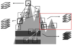
which we will call as group.This step is Block Matching(BM). Figure 2.31 can well

explain how we aregrouping.

Figure 2.31:grouping and collaborative thresholding

Collaborative filtering is a very important step in this algorithm. We will choose a 3D

transform or separable 2D+1D transform which is capable of utilizing the inter-fragment

and intra-fragment correlation and provide us with sparse representation.

Sparse representation is another very important aspect of this algorithm. Sparse

repre-sentation is to represent the data as coefficients such that most of the coefficient turns

to almost zero or zero. Sparse representation helps to reduce redundancy and express

correlation, we also want to detect the correlation between the pixels in the current

frag-ment and also between the current and reference fragfrag-ments. In this algorithm, after the

3D transform, we will hard-threshold the coefficients to get sparse representation. After

the hard-thresholding, we will inverse the 3D transform to get the spatial values from the

transformed coefficients. The process can be described by the following equation,

ˆ YSht

xR = τ

ht−1

3D (γ(τ ht

3D(ZSht

(45)

2.31. BM3D FirstStep 33

Here, γ is a hard-thresholding operator,τht₃_D is the 3D transform,τht₃_D−1 is the inverse 3D

transform, ˆYSht

xR is the 3D array of block-wise estimate we are getting after the

collabora-tive filtering.

• Aggregation: Now as we are considering overlapping blocks, we will have multiple

estimates for the same pixel. We will denote the final estimate of the first step as the basic

estimate for each of the pixels. We will perform aggregation to get the basic estimate for

each of the pixels. To find the basic estimate, ˆybasic _{for each of the pixel} _x_{, we will}

perform weighted average of the block-wise estimates ˆYSht

xR using the weights w

ht xR. If

we can reduce the effect of the estimate which is coming from of noisier block at times

of averaging, it is highly likely that we will get a better estimate. So, we will consider that a noisier block would have a larger sample variance. So, if we reward the estimate

coming from the noisier block with low weight, likely, we will get a better estimate. So,

we will consider our weight inverse proportionately to the total sample variance of the

corresponding block-wise estimates. Our considered weight can be understood by the

following equation,

whtxR=        1 σ2_NxR

har

, ifNxR

har ≥1

1, otherwise

      

Here,NxR

haris the number of non-zero coefficients after hard-thresholding. We can

calcu-late the basic estimate for each of the pixels by the following equation,

ˆ

ybasic(x)=

P

xRX

P

xmShtxR

wht_xRYˆxhtm,xR

P

xRX

P

xmSht_xR

wht_xRχxm(x)

,∀xX (2.32)

Here, χx_m : X → {0,1} is the characteristic function of the square support of a block

located atxmX, the blockwise estimates ˆYxhtm,xRare zero outside their support.

In the figure below, the left image is the actual cameraman image, the middle image is the

noisy cameraman image corrupted by Gaussian noise of mean 0 and standard deviation 10 and

(46)

(a) cameraman image (b) Noisy image (c) Denoised image

2.32 BM3D Second Step

After performing the first step, we have a basic estimate for all the pixels. We will denote this

image as the basic image.

• grouping and collaborative filtering: We will form the group of similar blocks in the

same as we have done in the previous step and can be expressed by following,

SwiexR =

||Yˆ_xRbasic−Yˆxbasic||22

(N₁wie)2 < τ

wie

match∀xX (2.33)

Here, ˆYxbasic is the considered current block of sizeN wie

1 ×N

wie

1 from basic image, ˆY

basic xR

is the reference block of same size ,Swie_xR is the set of all blocks which has normalized

squaredl2distance between ˆYbasic_xR and ˆYxbasic less than threshold,τ wie

match. Now, according

to the set, Swie_xR we will form two groups respectively from the basic image and noisy

image and denote them as following,

– Yˆbasic Swie

xR

by stacking together the basic estimate blocks ˆYbasic xSwie

xR

.

– ZSwie

xR by stacking together the basic estimate blocksZxSwiexR.

Let us define the Wiener shrinkage coefficients as following,

WSwien xR =

|τwie₃_D( ˆY_Sbasic xR )|

2

|τwie₃_D( ˆY_Sbasic xR )|

2+σ2 (2.34)

Here, WSwien

xR is the Wiener shrinkage coefficients for the setS

wien

xR . We will perform the

collaborative Wiener filtering of ZSwie

xR by element-by-element multiplication of the 3D

transform coefficientsτwie₃_D(ZSwie

(47)

2.32. BM3D SecondStep 35

WSwiexR. We will inverse transform to get actual coefficients from the transformed coeffi

-cients by following equation,τwie₃_D( ˆY_Sbasic

xR ) consists the 3D transform coefficients of ˆY

basic SxR .

ˆ Y_Swiewie

xR =

τwie−1

3D (WSwie xRτ

wie

3D(ZSwie

xR)) (2.35)

Now, ˆYwie

Swie_xR is thegroupof block-wise estimates.

• Aggregation: As we have considered overlapping blocks, we might have multiple

esti-mates for the same pixel. We can find the final estimate using the same procedure as we

have used in the aggregation portion of the first step. For this step, the weight we will use is following,

wwie_xR = σ−2||WSwie xR||

−2

2 (2.36)

Now, We will get the final estimate, ˆyf inal_{by a weighted average of the block-wise}

esti-mates, ˆYwie

Swie xR

using the weights described in the above equation for each of the pixels.

In the figure below, the left image is the actual cameraman image and the middle image is

the noisy cameraman image corrupted by Gaussian noise of mean 0 and standard deviation of

10 and the right image is the final denoised image by BM3D algorithm.

(a) cameraman image (b) Noisy image (c) Denoised image

Now, we will summarise the whole algorithm in simple steps,

1. Step 1. Getting the basic image

(a) Block-wise estimates:

i. grouping:

A. Find the blocks which are similar to the currently processing block

(48)

ii. Collaborative hard-thresholding:

A. Apply a 3D transform on thegroup.

B. In order to attenuate the noise, apply hard-thresholding on the transform

coefficients.

C. To produce estimates for allgrouped blocks, invert the transform

D. Return the estimates of the blocks to their original positions.

(b) Aggregation: Compute the basic estimate for all the pixels by weighted averaging

all of the obtained block-wise estimates that are overlapping.

2. Step 2. Final estimate: Use the basic image to perform grouping and collaborative Wiener filtering

(a) Block-wise estimates:

i. grouping:

A. Find the location of blocks that are similar to the current processing block.

B. Form twogroups using these locations, one from the basic image and one

from the noisy image.

ii. Collaborative Wiener filtering:

A. Apply a 3D transform on bothgroups.

B. Using the energy spectrum of the basic image as true energy spectrum for

Wiener filter, perform Wiener filtering on the noisygroup.

C. Apply inverse 3D transform on the filtered coefficients to produce final

estimates.

D. Return the estimates of the blocks to their original positions.

(b) Aggregation: Compute the final estimate for all the pixels by weighted averaging

all of the obtained block-wise estimates that are overlapping.

We will discuss the limitations of BM3D and some recent approaches to improve

perfor-mance in the next section.

2.33 Improvements of BM3D

Although BM3D shows better denoising performance than most of the denoising methods in

(49)

2.33. Improvements ofBM3D 37

years. The authors Dabov et al.[7] who proposed BM3D extended their algorithm for color

images [10].

Discrete cosine transform(DCT)[39][1] is representing the image in terms of sum of

dif-ferent cosine functions of different frequencies. Two-dimensional separable DCT possesses

very good energy compaction properties and is a very efficient transform in order to achieve

a sparse representation. However, if there are edges and singularities, then sparsity perfor-mance degrades[18]. So,the authors here [18] proposed to use the shape-adaptive

dct(SA-DCT)[37][38] to process the arbitrarily shaped image segments where the underlying signal

is uniform. SA-DCT has adaptive support and computed by cascaded application of

varying-length DCT transforms on the columns and on the rows respectively for the region. The authors

have utilized the Anisotropic Local Polynomial Approximation(LPA)-Intersection of

Confi-dence Intervals(ICI) [26][25][19] technique to decide the adaptive support. In this technique, a

varying-scale family of directional-LPA convolution kernels is used to produce a set of

direc-tional varying scale estimates for every specified direction. These estimates are then compared

by ICI rule to get an adaptive scale for every direction. These estimates altogether in an adap-tive convex combination provides us with the final anisotropic LPA-ICI estimate. Although

this work itself is a separate denoising algorithm we are discussing it here because the authors

later have used this approach with BM3D[8]. In this work, authors have decided the adaptive

support for the transform with LPA-ICI technique and used the SA-DCT as the 3D transform

of BM3D in both of the steps.

In order to improve the sparsity more, the authors proposed PCA on the adaptive shape

neighborhood decided by LPA-ICI technique in this paper [9] as a part of the employed

3-D transform. From groups of similar adaptive-shape neighborhoods, an empirical

second-moment matrix is formed and utilizing the eigenvalue decomposition of that matrix the PCA

bases are formed. Depending on a threshold, in some cases, the SA-DCT is used and for some

cases, the above mentioned PCA is used.

As the performance of BM3D degrades when the standard deviation of noise reaches 40, in

this paper [11] the authors proposed to combine tetrolet prefiltering with BM3D when the noise is strong. They have proposed to use tetrolet transform in the first step of BM3D to remove

part of the noise before Wiener filtering. Tetrolets are adaptive haar-type Wavelet filter bank

whose supports are the shapes called tetrominoes[27].

In this paper [17], after decomposing the bm3d restored image into three orthogonal

sub-bands, authors have observed that in the subband of the high-frequency component where the

Wavelet coefficients are less than a given threshold, some textures of the original image are

lost during denoising. Because of this loss, the Peak Signal to Noise Ratio(PSNR) in that band

Optimizing the usage of 2D and 3D transformations to improve the BM3D image denoising algorithm

Scholarship@Western

Scholarship@Western

Optimizing the usage of 2D and 3D transformations to improve

Optimizing the usage of 2D and 3D transformations to improve

the BM3D image denoising algorithm

the BM3D image denoising algorithm

Lay Summary

Contents

Chapter 1

Introduction

1.1

Motivations

1.2

Problem Statement

1.3

Our Objective

1.4

Thesis Contribution

1.5

Thesis Outline

Background Studies

2.1

Image Noise

2.2

Noise Types

2.3

Spatially Independent Noises

2.4

Gaussian Noise

2.5

Rayleigh Noise

2.6

Gamma Noise

2.7

Exponential Noise

2.8

Uniform Noise

2.9

Additive White Gaussian Noise

2.10

Spatially Dependent Noise

2.11

Speckle Noise

2.12

Impulse Noise

2.13

Our Considered Noise

2.14

Image Denoising

2.15

Spatial Filtering Methods

2.16

Linear Spatial Filters

2.17

Arithmetic Mean Filter

2.18

Minimum Mean Square Error(Wiener) Filtering

2.19

Non-linear Spatial Filter

2.20

Median Filter

2.21

Adaptive Median Filter(ADM)

2.22

Transform Domain Filtering Based Methods

2.23

Spatial Frequency Filtering

2.24

Wavelet Domain Filtering

2.25

Edge Guided Image Denoising

2.26

Total Variation (TV) Based Filtering

2.27

Anisotropic Di

ff

usion Filtering(ADF)

2.28

Non-local Means(NLM) Algorithm