Power System Short-Term Load Forecasting Using Artificial Neural Networks

(1)

IJEDR1602012

International Journal of Engineering Development and Research (www.ijedr.org)

78

Power System Short-Term Load Forecasting Using

Artificial Neural Networks

1_{Dr. Hassan Kuhba,}2_{Hassan A. Hassan Al-Tamemi} 1_{Assistant Professor,}2_{M. Sc.}

Electrical Engineering Department Engineering College/Baghdad University

________________________________________________________________________________________________________

Abstract - In this paper, a multi-layer perceptron with back-propagation algorithm as learning strategy is used to train the

neural networks. One of the important features of using (MLP) NNs is the weather variation such as temperature, humidity, cloudiness … etc., can be simulated as the most essential parameters that affect on the predicted load. The proposed method, by computation of the predicted loads for different parameters variations, is demonstrated on practical system (Iraqi National Grid, 14 load buses), and tested by 5-busses test system. The results of short-term load forecasting are obtained for on-line applications with high accuracy and reasonable error.

Keywords - Short –Term Electrical Load Forecasting (STLF), Artificial Neural Networks, Back propagation, Multi-Layer

perceptron.

________________________________________________________________________________________________________

I.INTRODUCTION

Load forecasting is an important component for power system energy management system. Precise load forecasting helps the electric utility to make unit commitment decisions, reduce spinning reserve capacity and schedule device maintenance plan properly [1]. Besides playing a key role in reducing the generation cost, it is also essential to the reliability of power systems. The system operators use the load forecasting result as a basis of off-line network analysis to determine if the system might be vulnerable. If so, corrective actions should be prepared, such as load shedding, power purchases and bringing peaking units o n line. Since in power systems the next days’ power generation must be scheduled every day, day-ahead short-term load forecasting (STLF) is a necessary daily task for power dispatch. Its accuracy affects the economic operation and reliability of the system greatly. Under prediction of STLF leads to insufficient reserve capacity preparation and, in turn, increases the operating cost by using expensive peaking units. On the other hand, over prediction of STLF leads to the unnecessarily large reserve capacity, which is also related to high operating cost. It is estimated that in the British power system every 1% increase in the forecasting error is associated with an increase in operating costs of 10 million pounds per year [2]. In spite of the numerous literatures on STLF published since 1960s, the research work in this area is still a challenge to the electrical engineering scholars because of its high complexity. How to estimate the future load with the historical data has remained a difficulty up to now, especially for the load forecasting of holidays, days with extreme weather and other anomalous days. With the recent development of new mathematical, data mining and artificial intelligence tools, it is potentially possible to improve the forecasting result.

With the recent trend of deregulation of electricity markets, STLF has gained more importance and greater challenges. In the market environment, precise forecasting is the basis of electrical energy trade and spot price establishment for the system to gain the minimum electricity purchasing cost. In the real-time dispatch operation, forecasting error causes more purchasing electricity cost or breaking-contract penalty cost to keep the electricity supply and consumption balance. There are also some modifications of STLF models due to the implementation of the electricity market. For example, the demand-side management and volatility of spot markets causes the consumer’s active response to the electricity price. This should be considered in the forecasting model in the market environment. Load forecasting is one of the central functions in power systems operations. The motivation for accurate forecasts lies in the nature of electricity as a commodity and trading article; electricity cannot be stored, which means that for an electric utility, the estimate of the future demand is necessary in managing the production and purchasing in an economically reasonable way [3].

II.ELECTRICALLOADFORECASTING

Load forecasting in power system is an important subject and has been studied from different point of view in order to achiev e better load forecasting results [4]. Techniques such as regression analysis, expert system, artificial neural network and multi-objective evaluations has been used based on different choices of inputs and available information. Distribution system load forecasting has been challenging problem due to its spatial diversity and sensitivities to land usage and customer habits. Different tools have been developed to assist utilities to simulate and estimate the future land, usage land and load growth in their territory, so that distribution system planners can plan according to their goal and interests. Many factor need to be considered for this purpose, namely,

 What type of land usage will be in their territory in the future?  What type of power consumption will be in their territory?

(2)

IJEDR1602012

79

Load forecasting is an essential tool for operation and planning of power system. It is required for unit commitment, energy transfer scheduling and load dispatch. The different types of load forecasting [5] can be classified according to forecast period as:

a. Short –term load forecasting (STLF), which are usually from one hour to one month. It is important for various applications

such as unit commitment, economic dispatch, energy transfer scheduling and real time control. A lot of studies have been done for using of short-term load forecasting [5] with different methods. Some of these methods may be classified as follow: Regression, Kalman filtering, Box &Jenkins model, Expert system, Fuzzy inference, Neuro-fuzzy models and Chaos time series analysis. Some of these methods have main limitations such as neglecting of some forecasting attribute condition, difficulty to find functional relationship between all attribute variable and instantaneous load demand, difficulty to upgrade the set of the rules that govern at expert system and disability to adjust themselves with rapid nonlinear system –load change. The NNs can be used to solve these problems. Most of these projects using NNs considered many factors such as weather condition, holidays, weekends and special sport matches days in forecasting model, successfully. This is because of learning ability of NNs with many input factors.

b. Medium-term load forecasting (MTLF) , which are usually from month to a year, used to purchase enough fuel for power

plant after electricity tariffs are calculated [6].

c. Long-term load forecasting (LTLF), which are longer than a year, used by planning engineers economists to determine the

type and the size of generating plants that minimize both fixed and variable costs [7].

The system load of an area is dependent on its industrial, commercial and agricultural activities as well as its weather condition [8]. Special events on religious and social occasions also add-up a component to the system load on particular days. The portion of the demand which is found to be dependent the overall economic activities and climatic condition of an area is known as the base load of the system. Superimposed on this base load is a demand which can be attributed to the fluctuations of the weather

condition from normalcy and special events. Thus the demand D at any instant consist of the following components,

D = L+W+C (1)

Where L is the base load, W the weather-dependent component and C represents the part which is due to some festival or event. The meteorological factors which are responsible for the weather-Sensitive component of load are temperature, humidity, cloudiness, wind velocity… etc. An increase or decrease of temperature above or below the normal causes an increased consumption of electricity due to operation of the cooling / heating component and thus the demand shoots up beyond the base load. Cloudiness during the daytime affects the visibility and hence the customers' demand increases. Similarly the wind velocity has a bearing on the traction load.

III.CHARACTERISTICSOFPOWERSYSTEMLOAD

The system load is the sum of all the consumers’ load at the same time. The objective of system STLF is to forecast the future system load. Good understanding of the system characteristics helps to design reasonable forecasting models and select appropriate models in different situations. Various factors influence the system load behavior, which can be mainly classified into the following categories

● Weather ● Time ● Economy

● Random disturbance.

IV.ARTIFICIALNEURALNETWORKS

(3)

IJEDR1602012

80

powerful technique to solve many real world problems. They have the ability to learn from experience in order to improve their performance and to adapt themselves to changes in the environment. In addition to that, they are able to deal with incomplete information or noisy data and can be very effective especially in situations where it is not possible to define the rules or steps that lead to the solution of a problem. They typically consist of many simple processing units, which are linked together in a complex communication network.

V.LEARNINGTHENEURALNETWORKS

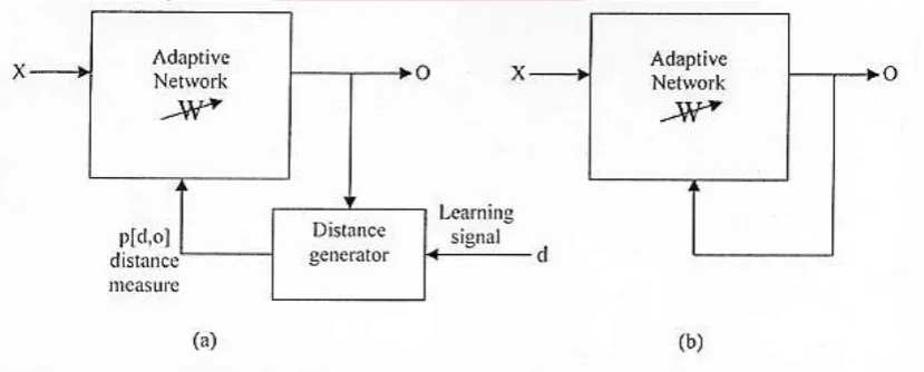
The learning algorithm is a procedure for modifying the weight on the connection links in neural network, also known as training algorithms or learning rule. Training is accomplished by sequentially applying input vector, while adjusting network weights is done according to pre-determined procedure. During training, the network weight gradually converges to a value, so that each input vector produces the desired output vector. The network becomes more knowledgeable about its environment after each iteration of learning process. All learning methods used for adaptive neural network can be classified into two major categories as shown in Fig.1:

Supervised Learning

Which is a process of adjusting the weights in a neural net using a learning algorithm; the desired output for each of a set of training input vectors is presented to the net. The network then processes the inputs and compares its resulting outputs against the desired outputs. Errors are then propagated back through the system, causing the system to adjust the weights which control the network. Much iteration through the training data may be required. When the input is applied the desired response of the system is provided by a teacher. The distance between the actual and the desired response serves as an error measure and is used to correct network parameters externally (weights). Adjusting the weight, the teacher may implement a reward and punishment scheme to adapt the network weight matrix.

Unsupervised Learning

The network has no feedback on the desired or corrected output. There is no teacher to present desired patterns. It is also referred to a self-organization, it is expected to organize itself into some useful configuration, and recall the weights to produce output vector that are consist within the network. Learning must somehow be accomplished based on .observation of response to input that has marginal or no knowledge about.

Fig.1 Schematic diagram of adaptive weight: (a)Supervised learning, (b) Unsupervised learning

BACK PROPAGATION ALGORITHM

Back-propagation is a supervised learning technique used for training artificial neural networks. It was first described by Paul Werbos in 1974, and further developed by David E. Rumelhart, Geoffery E. Hinton and Ronald j. Williams in 1986. It is most useful for feed-forward networks (networks that have no feedback, or simply, that have no connections that loop). The term is an abbreviation for "backwards propagation of errors". Back-propagation requires that the transfer function used by the artificial neurons (or "nodes") be differentiable. Back propagation networks are among the most popular and widely used neural networks because they are relatively simple and powerful. Back propagation was one of the first general techniques developed to train multi-layer networks, which does not have many of the inherent limitations of the earlier, single -layer neural nets criticized by Minsky and Papert.These networks use a gradient descent method to minimize the total squared error of the output. A back propagation net is a multilayer, feed forward network that is trained by back propagating the errors using the generalized Delta rule. The input is the input to the hidden layer and the output layer is the output from the immediate previous layer, so it is called feed forward neural network. The number of the input units and the output units are fixed to a problem, but the choice of the number of the hidden units is somehow flexible. Too many hidden units may cause over fitting, but if the number of hidden units is too small, the problem may not converge at all. Usually a large number of training cases may allow more hidden units if the problem requires so.

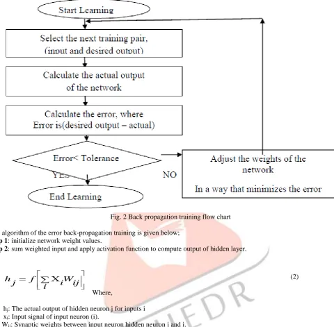
VI.TRAININGABACK-PROPAGATIONNETWORK

(4)

IJEDR1602012

81

Fig. 2 Back propagation training flow chart

The algorithm of the error back-propagation training is given below;

Step 1: initialize network weight values.

Step 2: sum weighted input and apply activation function to compute output of hidden layer.

(2) Where,

hj: The actual output of hidden neuron j for inputs i xi: Input signal of input neuron (i).

Wij: Synaptic weights between input neuron hidden neuron j and i. ƒ: The activation function.

Step 3: sum weighted output of hidden layer and apply activation function to compute output of output layer.

(3)

Where, Ok: The actual output of output neuron k.

Wjk: Synaptic weight between hidden neuron j and output neuron k.

Step 4: compute back propagation error.

(4) Where,

f’′:The derivative of the activation function.

dk: The desired of output neuron

Step 5: calculate weight correction term.

 











1 



W

_jk

n



_k

h

_j



W

_jk

n

(5) where, η: is the learning ratio and α: is the moment coefficient

Step 6: sums delta input for each hidden unit and calculate error term

    

  

 



i

ij

W

i

f

j

h

















j

jk j

k

f

h

W

O



k k



(

_o

_K

)

k



d



O

f



(5)

IJEDR1602012

82 



















k i ij i jk k

j



W

f

X

W



(6)

Step 7: calculate weight correction term.

 











1 



W

_ij

n



_j

X

_i



W

_ij

n

(7)

Step8: update weights



n

1 

W

(

n

)

W

(

n

)

W

_jk





_jk





_jk (8)

(9)

Step 9: repeat step2 for given number of error



















p k

p

k

O

p

k

d

p

MSE

(

)

2

1

(10)

Where, p: The number of patterns in the training set and MSE is the mean square error.

Step 10: END

VII.NEURALNETWORKSBASEDSTLF

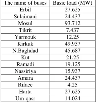
In the current study, neural networks are used to fit a set of experimental points in order to provide a purely empirical model. The experimental points are called the training cases (or learning cases) and another are called testing cases. They consist of input vectors (values of input variables) associated with the experimental output value. To solve a problem with aback-propagation network, it is shown sample inputs with the desired outputs, while the network learns by adjusting its weights. If it solves the problem, it would have found a set of weights that produce the correct output for every input. The inputs to the network need to contain sufficient information pertaining to the target, so that there exist relating correct outputs to inputs with the desired degree of accuracy. This work is tested by using 5-busses test system, and applied on symbol of Iraqi national grid fourteen busbars to forecast the load for each one for one month in winter. The name of buses and its basic load at normal temperature 20 C˚ and blue sky 132KV is illustrated in table (1). ANNs can only perform what they were trained to do. As for the case of STLF, the selection of the training set is a crucial one. The criteria for selecting the training set is that the characteristics of all the training pairs in the training set must be similar to those of the day to be forecasted. Choosing as many training pairs as possible is not the correct approach for the following reasons:

1. Load periodicity. The 7 days of a week have rather different patterns. Therefore, using Sundays' load data to train the network which is to be used to forecast Mondays' loads would yield wrong results.

2. Because loads possess different trends in different periods, recent data is more useful than old data. Therefore, a very large training set which includes old data is less useful to track the most recent trends. As discussed in 1), to obtain good forecasting results, day type information must be taken into account.

In all, because of the great importance of appropriate selection of the training set, several day type classification methods are proposed, which can be categorized into two types. One includes conventional method which uses observation and comparison. The other, is based on unsupervised ANN concepts and selects the training set automatically.

Table (1) the name of busbar and its basic load The name of buses Basic load (MW)

Erbil 27.625

Sulaimani 24.437

Mosul 93.712

Tikrit 7.437

Yarmouk 12.25

Kirkuk 49.937

N.Baghdad 45.687

Kut 21.25

Ramadi 19.125

Nassiriya 15.937

Amara 24.437

Rifaee 4.25

Harta 27.625

Um-qasr 14.024

)

(

)

(

)

1

(6)

IJEDR1602012

83

In this study there are two input parameters to every one of the above bas bar, temperature and weather. The weighting factors used by Philadelphia Electric Co. of USA to assess the weather-dependent load of their system due to fog and cloudiness during the day time are used to choose the historical load. The above mentioned company also used a correction factor of 2% for every 5C˚ variation in temperature from the normal temperature of the month, established by weather experts.

VIII.BACKPROPAGATIONSTRUCTURE

In this work, a multilayer neural network has been used, as it is effective in finding complex non-linear relationships. It has been reported that multilayer ANN models with only one hidden layer are universal approximates. Hence, a three layer feed forward neural network is chosen as a correlation model. The weighting coefficients of the neural network are calculated using MATLAB programming. Structure of artificial neural network built as:

1. Input layer: A layer of neurons that receive information from external sources and pass this information to the network for

processing. These may be either sensory inputs or signals from other systems outside the one being modeled. In this work two input neurons in the layer and there is a set of (35) data points available of the training set.

2. Hidden layer: A layer of neurons that receives information from the input layer and processes them in hidden way. It has no

direct connections to the outside world (inputs or output). All connections from the hidden layer are to other layers within the system. The number of neuron in the hidden layer chosen (trial and error) for this network is seven neurons.Determination the optimal number of hidden neurons is a crucial issue. If it is too small, the network cannot posse’s sufficient information, and thus yields inaccurate forecasting results. On the other hand, if it is too large, the training process will be very long. The best number of hidden neurons depends in a complex way on:

 the numbers of input and output units  the number of training cases

 the amount of noise in the targets

 the complexity of the function or classification to be learned etc

In most situations, there is no way to determine the best number of hidden neurons without training several networks and estimating the generalization error of each.

The number of input units and output units are fixed to a problem, but the choice of the number of the hidden units is flexible. The number of hidden layer neuron should be as minimum (2N+1); here N is the number of input neurons.

3. Output layer: A layer of one neuron that receives processed information and sends output signals out of the system.

4. Bias: The function of the bias is to provide a threshold for activation of neurons. The bias input is connected to each of hidden

(7)

IJEDR1602012

84

for Erbil busbar

IMPLEMENTATION RESULTS

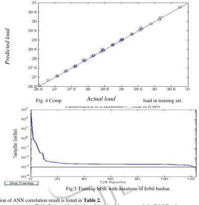
The network architecture used for prediction the load in Erbil bus bar illustrated in Fig.3 consist of two inputs neurons corresponding to the state variables of the system, with seven hidden neurons and one output neuron. All neurons in each layer were fully connected to the neurons in an adjacent layer. Resulting in (21) connection links, (7) of which bias links. Fig. 4

compares the predicted load with actual load for training set. Epochs are usually increased in ANN to make the network repeatedly understand the trends of the data. Fig.5 illustrates the number of epochs with MSE for Erbil busbar

Fig. 4 Comparison between the predicted and actual load in training set.

Fig.5 Training MSE with iterations of Erbil busbar. The prediction of ANN correlation result is listed in Table 2.

Table 2. Actual load and predicted load for one month for Erbil Bus-bar. Days Actual load A

(MW)

Predicted load P (MW)

1 29.603 28.7337

2 29.890 29.0446

3 30.178 29.3244

4 30.752 29.5833

5 31.040 30.2206

6 31.635 30.7529

7 29.022 28.1103

8 29.304 28.4633

9 29.585 28.7599

10 30.149 29.0096

11 30.431 29.2987

12 30.994 30.0926

13 28.453 27.5727

14 28.730 27.9084

15 29.006 28.1820

16 29.558 28.4330

Pre

dicte

d load

(8)

IJEDR1602012

85

17 29.835 28.7216

18 30.387 29.5274

19 27.884 27.0505

20 28.154 27.3655

21 28.425 27.6221

22 28.967 27.8617

23 29.237 28.1459

24 29.779 28.9443

25 27.326 26.5455

26 27.592 26.8353

27 27.857 27.0691

28 28.388 27.5625

29 28.653 27.9225

30 29.184 28.3653

The ANN also tested with 5-busses test system, B1and B2 are generation busses B3, B4and B5are load busses. We will take B3 as example to explain the test result. The same procedure that applied on Iraqi National Grid is applied here. Fig.6 illustrate the number of epochs with MSE for B3bus bar. Fig. 7 compares the predicted load with actual load. The prediction of ANN correlation result is listed in Table. 3.

Fig. 6. Training MSE with iterations of B3 bus bar

Fig. 7. Comparison between the predicted load and actual load of B3bus bar Table 3. Actual load and predicted load for one month for B3 busbar

Pre

dicte

d

(9)

IJEDR1602012

86

Days Actual load A

(MW)

Predicted load P (MW)

1 46.818 46.7979

2 47.286 47.2459

3 47.754 47.6998

4 48.222 48.1715

5 48.690 48.6728

6 49.158 49.1660

7 45.900 45.9183

8 46.359 46.3686

9 46.818 46.8077

10 47.277 47.2620

11 47.736 47.7330

12 48.195 48.2262

13 45.000 45.0004

14 45.45 45.4589

15 45.900 45.8873

16 46.350 46.3277

17 46.800 46.7846

18 47.250 47.2570

19 44.100 44.0907

20 44.541 44.5424

21 44.982 44.9690

22 45.423 45.3970

23 45.864 45.8420

24 46.305 46.3034

25 43.218 43.2260

26 43.650 43.6478

27 44.082 44.0845

28 44.514 44.5026

29 44.946 44.9366

30 45.378 45.3882

IX.CONCLUSION

The general objective of this work is to provide power system dispatchers with an accurate and convenient short-term load forecasting (STLF) system, which helps to increase the power system reliability and reduce the system operation cost. From the implementations of the proposed method, we conclude the following:

1. Among other methods of short-term load forecasting, the artificial neural networks have established as a promising tool in power system load forecasting problem solution.

2. The weather variation such as temperature, humidity, cloudiness, fogs … etc., can be emulated with Artificial Neural Networks whereas conventional methods cannot simulate the above factors.

3. The solution of STLF using Multi-layer perceptron with back-propagation algorithm was achieved in a very short computing time, so it can be implemented for on-line applications.

4. Neural computing has attractive features such as its robustness in dealing with incomplete or bad data by reprocessing the input information.

5. The demonstration of the proposed method on Iraqi National Grid practical system and 5-busses test system was shown high accuracy results with very reasonable error.

X.REFERENCES

[1] Jingfei Yang, 2006, ″power system Short-term load forecasting″, Ph.D. Thesis, Der Technischen University Darmstadt.

[2] G. Gross, F. D. Galiana, ″Short-term load forecasting″, Proceedings of the IEEE, 75(12), 1987, pp. 1558 – 1571.

[3] Pauli Murto, ″Neural Network models for short-term load forecasting″, M.Sc. Thesis, Helsiki University of Technology, January 1998.

[4] Mo-yuen Chow and Hahn Tram, ″Methodology of Urban Re-Development Consideration in Spatial Load Forecasting″, IEEE Transactions on Power Systems, Vol. 12, No. 2, May 1997.

[5] M.Tarafdar Haque and A.M.Kashtiban, ″Application of Neural Networks in Power System; A Review″, Transactions on Engineering, Computing and Technology, Vol. 6, June 2005, ISSN1305-5313.

[6] M. Gavrilas, I. Ciutera and C. Tanasa , ″Medium-Term Load Forecasting with Artificial Neural Network Models″, IEE Cried Conference, June 2001, pp. 482-486.

[7] M.S. Kandil, S.M. El-Debeiky and N.E. Hasasien, ″Long –Term Load Forecasting for Fast Developing Utility Using a Knowledge-Based Expert System″, IEEE Trans. on Power Systems, Vol. 17, No. 2, May 2002, pp. 491-496.

(10)

IJEDR1602012

87

[9] H.S Hippert, C. E. Pedreira, and R. C. Souza, ″Neural Network for Short –Term load Forecasting: A Review and