University of South Carolina
Scholar Commons
Theses and Dissertations
1-1-2013
Modeling Approaches, Physiological Responses,
and Climate Change: How Good is "Good
Enough?"
Nicole KishUniversity of South Carolina
Follow this and additional works at:https://scholarcommons.sc.edu/etd Part of theLife Sciences Commons
This Open Access Thesis is brought to you by Scholar Commons. It has been accepted for inclusion in Theses and Dissertations by an authorized administrator of Scholar Commons. For more information, please [email protected].
Recommended Citation
i
MODELING APPROACHES, PHYSIOLOGICAL RESPONSES, AND CLIMATE CHANGE: HOW GOOD IS “GOOD ENOUGH?”
By
Nicole E. Kish
Bachelor of Science
University of South Carolina, 2012
Submitted in Partial Fulfillment of the Requirements
For the Degree of Master of Science in
Marine Science
College of Arts and Sciences
University of South Carolina
2013
Accepted by:
Brian Helmuth, Major Professor
David Wethey, Committee Member
Claudia Benitez-Nelson, Committee Member
ii
ACKNOWLEDGEMENTS
I received assistance from many people during the course of my research. I am
grateful to my adviser, Brian Helmuth, for his guidance and insight into expanding my
research. David Wethey helped to streamline my research question and presentation and
provided insight into the technical details regarding how to conduct my research. Claudia
Benitez-Nelson provided support regarding the presentation and interpretation of my
analyses. Sally Woodin also provided insight and ideas. I am grateful to Evan Kodra and
Greg Carbone regarding their insight into the realm of forecast verification, and to
Nirnimesh Kumar for assistance with programming in Matlab. I would also like to thank
the Helmuth lab (Mackenzie Zippay, Cristian Monaco, Shadow Gulledge, Nick Colvard,
iii ABSTRACT
Predicting spatial and temporal patterns in the responses of organisms and
ecosystems to climate change has emerged as a major focus of macrophysiological
research, with much work centered on the impacts of temperature. A potential difficulty
lies in the observation that measures of “habitat” such as air, land and sea surface
temperature often differ greatly from the body temperature actually experienced by
organisms, as the latter drives reproduction and survival. As a result, it is unclear how
often these simple measurements of habitat are “good enough” for predicting
physiological stress in the field, and when more complicated methods are needed. Using
a dataset of body temperatures of rocky intertidal mussels, I compared the predictive
capacity of four methods for mapping patterns of physiological stress at five sites along
the west coast of the United States. Using a thermal physiology framework, I divided
predicted and measured temperatures into lethal, suboptimal (both too hot and too cold)
and optimal categories. Results suggest that while the various methods have similar
accuracy (skill) when compared using common metrics such as Root Mean Square Error,
they differ significantly in their ability to predict physiological responses, especially
extremely high temperatures. My results emphasize that tests of model skill need to be
matched to physiologically meaningful metrics when attempting to predict patterns of
iv
TABLE OF CONTENTS
Acknowledgements…...………..ii
Abstract………...iii
List of Tables………...………...….v
List of Figures……….…………vi
Introduction………..1
Chapter 1………12
1.1 Introduction……….13
1.2 Methods………...17
1.3 Results……….27
1.4 Discussion………...31
Tables……….36
Figures………38
Conclusion……….42
v
LIST OF TABLES
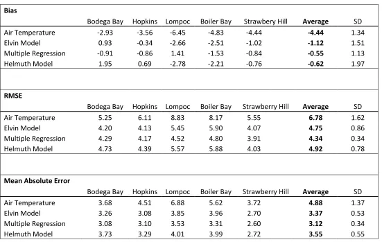
Table 1.1 Bias, RMSE, and MAE of all models at all sites………..36
vi
LIST OF FIGURES
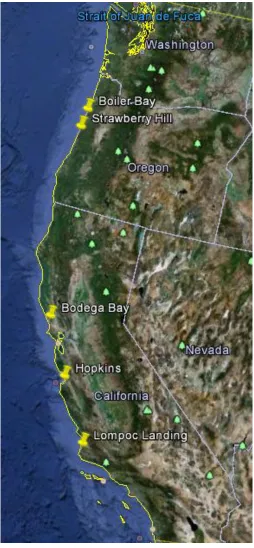
Figure 1.1 Location of study sites……….38
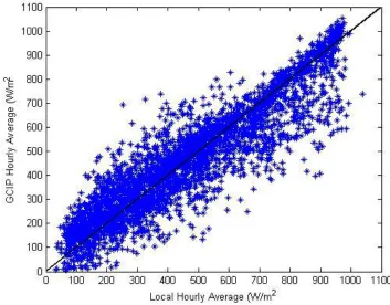
Figure 1.2 Comparison of local and gridded solar radiation data………39
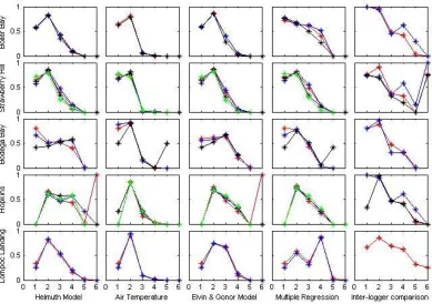
Figure 1.3 Hit rates for all models at all sites………...40
1
INTRODUCTION
Due to greenhouse gas emissions resulting from anthropogenic activities, global
surface air temperatures have been increasing since the mid-19th century. Changes in the
hydrologic cycle, wind and precipitation patterns, and the duration and intensity of
extreme heat events are predicted to accompany the warming trend (IPCC, 2007). As
surface, air and sea temperatures warm, species ranges are predicted to shift poleward,
toward higher altitudes (Walther et al., 2002; Parmesan & Yohe, 2003) or into less
thermally stressful refuges (Helmuth et al., 2002). Since some warming would still take
place even if greenhouse gas emissions were stabilized (IPCC, 2007) accurately
predicting the effects the changing climate will have on species is imperative to
understanding future species distributions and changes in ecosystem function.
Specific physical factors limit the physiological performance and survival of all
organisms—taken together, these factors comprise the axes of Hutchinson’s niche, or
“n-dimensional hypervolume” within which a species can survive (1957). Hutchinson
further divided the concept into that of the “fundamental niche” which accounted for
limits set only by physical parameters (and the organism’s physiological tolerance of
those parameters), and the “realized niche,” which included the effects of biotic
interactions such as competition and predation. Here I focus on the concept of the
fundamental (physiological) niche, although changes in the extent of one organism’s
fundamental niche may affect another’s realized niche as a result of biotic interactions.
1
potentially future extent of habitat suitable for a particular organism (Kearney, 2006).
Since external conditions interact with an organism’s behavioral, morphological, and
physiological traits, two species exposed to the same environment can experience very
different levels of physiological stress, i.e. exist at different locations within their
respective niche (Kearney 2006, Kearney et al., 2010). Moreover, two organisms with
similar physiological tolerances can also experience different levels of stress- and live
within different regions of their respective niche spaces- as a result of differences in how
“habitat” (such as air and surface temperature) are translated into conditions more
relevant to the organism’s physiology, such as body temperature. Since the
Hutchinsonian niche concept is in essence a property inherent to a particular organism,
rather than that organism’s environment, Kearney suggests that the term “niche” be
reserved only for mechanistic interactions between organism and environment, and
“habitat” used to refer to parameters that describe the physical nature of an the region the
organism occupies (Kearney, 2006), regardless of how that habitat is perceived at a
physiological level by each species. I use these definitions throughout the remainder of
this paper.
Since temperature has long been shown to influence a wide variety of
physiological processes (e.g.; Somero, 2002; Denny, 2011; Huey & Kingsolver, 2011),
climate change will alter the extent of an organism’s fundamental niche in space and
time. Physiological responses to temperature are represented by thermal performance
curves, the breadth of which represents fundamental thermal niche width (Huey &
Stevenson, 1979; Roughgarden, 1972). Performance curves are often asymmetric around
2
gradually declines; as temperatures rise above optimum, performance drops off sharply
(Huey & Stevenson, 1979). Therefore, even a relatively small increase of only a few
degrees in temperature may result in a sharp decline in physiological performance when
the organism is already living at or slightly above its optimal body temperature. Because
of this asymmetric nature of performance curves, organisms are predicted to center their
body temperature range at a value slightly below optimal when they experience a range
of temperatures, in order to maximize total fitness (Martin & Huey, 2008).
Frequently, changes in a species thermal niche are predicted by correlating
species presence data with a single environmental parameter, quite often air temperature,
and forecasting or hindcasting changes in abundance (e.g. Lesser et al., 2010; Firth et al.,
2011). Because these correlative models rely on data taken at the “habitat” level, they do
not account for the mechanisms by which environmental conditions are translated into
physiological stress and as a result can be problematic, especially when applied to novel
climatic conditions (Kearney et al., 2008). For example, because convection by wind can
cool organisms exposed to solar radiation, an organism with a morphology that enhances
turbulence may experience a lower body temperature than one that is more “streamlined”
even when both organisms are exposed to precisely the same conditions of weather. As a
result, it has been suggested that commonly used metrics of “habitat temperature” such as
air or surface temperature may not effectively represent body temperature, which
ultimately controls physiological performance.
The parameters that define the fundamental niche vary temporally: both
short-term, infrequent exposures to extremes and prolonged or repeated exposures to sublethal
3
2011). Extreme events themselves may not necessarily be caused by extremes in any one
particular aspect of the environment, but rather the simultaneous occurrence of several
stressors which interact synergistically (Denny et al, 2009), such as elevated air
temperature and maximal levels of solar radiation (Marshall et al. 2010). Temporal
non-coincidence of sublethal stressors can also affect physiological performance, since they
do not allow for a period of recovery (Pincebourde et al., 2012). In this instance,
correlative approaches using a single climatic variable do not account for interactions
between these drivers, especially if a non-climatic factor is of importance (Marshall et al.,
2010).
Other approaches seek to overcome these drawbacks. Mechanistic niche models,
though significantly more complex than correlative models as they require extensive
parameterization and detailed knowledge of the characteristics of both organism and
environment, can potentially more accurately predict the effects of climate change as they
account for the means by which environmental parameters are translated into
physiologically relevant characteristics (Kearney, 2006; Kearney et al, 2010). For
example, a mechanistic model designed to predict the fundamental thermal niche as a
function of body temperature will account for the sources, sinks, and stores of heat within
the organism (Porter & Gates 1969; Helmuth, 1998). Heat may be gained from short
wave solar radiation; gained or lost due to radiation with the sky, radiation with the
ground, conduction with the ground, and convection with the surrounding air; and lost
due to evaporative cooling. By accounting for the ways in which an organism’s traits
4
a mechanistic niche model will predict stored heat within an organism, which in turn
determines body temperature (Porter & Gates 1969; Helmuth, 1998).
An example of the complexity involved in predicting physiological stress due to
climate is body temperature of intertidal ectotherms, since these organisms must contend
alternatively with terrestrial and marine conditions. Body temperature—the factor
responsible for stress—of intertidal ectotherms is driven by multiple aspects of the
environment, such as air temperature, water temperature, solar irradiance, wave splash,
wind speed, and the timing of the tides (Helmuth 1998, 1999; Helmuth et al., 2002) and
often differs greatly from the temperature of the ambient air or water (e.g. Southward,
1958; Lewis, 1963; Etter, 1988; Helmuth, 1998). As a result, body temperatures of these
organisms are believed to frequently approach the physiological limits of their species
(Somero, 2002). Because their survival is so closely tied to aspects of the physical
environment, intertidal ectotherms may be especially vulnerable to the changes brought
about climate change and can serve as an effective tool for predicting its effects (Denny
& Harley 2006).
In order to accurately predict the effects of a change in body temperature on
species distributions and ecosystem function, models must be grounded in a physiological
framework; i.e., they must account not only for the conditions an organism experiences
but where those conditions place it along its performance curve or within its fundamental
niche. During stressful conditions, organisms make potentially ecologically-significant
trade-offs, such as reallocating energy used for processes such as reproduction and
growth towards energetically costly defense and repair mechanisms (Petes et al., 2008).
5
to protein damage (e.g. Helmuth & Hofmann, 2001), diminished growth, and decreased
energy allocated to reproduction (e.g. Petes et al., 2007). Predictions of the effects of a
changing climate must account for changes in ecosystem function due to sublethal stress
as well as changes due to mortality.
A central problem facing climate scientists is how to quantify the accuracy of
imodels, especially when forecasting future responses under what will likely be novel
conditions. Several studies have attempted to compare mechanistic (process-based)
models against correlative models (e.g. Buckley et al. 2010). Yet, a key assumption in
these comparisons is that the metric being used to test accuracy is biologically relevant.
For example, mechanistic models that use weather data collapsed into monthly averages
may fail for the same reason as correlative approaches (Kearney et al. 2012). As a result,
they may appear to perform with similar accuracy to correlative models (Buckley et al.
2010) when in reality both are failing to account for the role of high frequency variation
in body temperature (Kearney et al. 2012).
I tested the predictive capacity of four methods for quantifying body temperature
(and thus, thermal stress) of the California mussel, Mytilus californianus. In situ body
temperatures of living mussels were collected by biomimetic sensors deployed at five
sites spanning ten degrees of latitude along the west coast of the United States. Using a
thermal physiology framework, I divided both measured and predicted temperatures into
categories of optimal, suboptimal (in terms of both heat and cold stress), and lethal
conditions. I analyzed the overall ability of each method to predict body temperature
using both common statistical metrics such as Root Mean Squared Error, but in addition-
6
capture the physiological stress experienced by mussels. I hypothesized that simple
metrics of the environment such as air temperature might be sufficient for predicting
average conditions. However, because high body temperatures have been shown to differ
significantly from the temperature of the mussel’s surroundings, I hypothesized that
mechanistic models would be necessary to predict extreme (and ecologically significant)
events.
1.1.1 Model stationarity
Both correlative and mechanistic approaches assume “model stationarity,” i.e. that
models developed and tested in one location and/or time can be applied to different
geographic regions and future conditions. This assumption is based on the idea of “niche
conservatism,” that the limitations on the fundamental niche remain constant over time. It
also assumes that the mechanisms setting limits in the region being tested are the same as
those in the location for which the model is being applied. Such an assumption may be
faulty because, for example, both lethal extremes and chronic exposure to sublethal
extremes that ultimately result in death or reproductive failure have been shown to set
range limits (Wethey et al. 2011a, Woodin et al. 2013). Thus, while the validity of the
model stationarity assumption is essential for accurately predicting the effects of climate
change biogeographic models have been observed to fail when applied to novel
conditions (Woodin et al., 2013). Even mechanistic models may not accurately reflect
body temperatures at sites other than the ones for which they were developed (e.g.
7
The models used in this study aim to predict body temperature from habitat-level
measurements; thus, failure of these models at certain locations would not imply a
fundamental niche shift or changes in the mechanism by which distribution is limited.
Instead, it would indicate inability to accurately reflect the interaction between
environment and organism at that site.
I explored the concept of model stationarity in space by performing analyses at
five different sites spanning ten degrees of latitude on the west coast of the United States
and varied the level of site-specificity in the models I chose. One model, developed by
Elvin & Gonor (1979) was developed and tested only for one particular site; however, I
applied this model to all five sites without modification. I used a general biophysical
model (Helmuth et al., 2011), developed at one particular site and applied to others, to
generate predictions of body temperature. The use of air temperature as a proxy was also
intended to be a general approach applicable to all sites. Finally, I used a multiple
regression approach to create simple models tailored to each particular location. The aim
of this approach was to investigate any potential patterns in geography that might lead to
model failure at one site as opposed to another.
1.1.2 Ecology of Mytilus californianus
The California mussel, Mytilus californianus, is a sessile invertebrate that inhabits
rocky shores of North America, whose range extends from Alaska to Baja California
(Smith et al, 2006), and whose ecology has been extensively studied. It is competitively
dominant throughout the mid-intertidal zone, with predation from the seastar Pisaster
8
temperature stress restricting coupled with reduced feeding time assumed to limit its
upper intertidal limit (Seed & Suchanek, 1992). M. californianus uses byssus threads to
attach to hard substrata and others of it species, thus providing structure and stability to
the intertidal ecosystem (Smith et al. 2006; Zippay & Helmuth, 2012). This species of
mussel does not have a distinct spawning season, but instead “dribbles” gametes
throughout the year (Seed & Suchanek, 1992).
The ability of M. californianus to behaviorally regulate its body temperature is
limited, as it cannot move to a less-thermally stressful location, and laboratory
experiments have demonstrated little effect of gaping behavior on the body temperature
of these organisms (Fitzhenry et al, 2004). Optimal temperatures for this species range
from 17° to 22°C (Bayne et al, 1976). Exposure to freezing conditions is lethal (Seed &
Suchanek, 1992), and Denny et al. (2011) report the LT50 (temperature at which 50%
mortality is observed) for M. californianus as 38.2° C, with 100% mortality when body
temperatures exceed 41°C. During periods of aerial exposure, the body temperature of
M. californianus has been observed to regularly exceed 30°C (e.g. Elvin & Gonor, 1979).
Thermal stress in this species does not increase with decreasing latitude along the Pacific
coast of the US; midday low tides, during which mussels are exposed to the “harshest”
terrestrial conditions, occur more frequently during the summer at northern sites in
Washington and Oregon than at southern sites in California (Helmuth et al, 2002), and
“risky” days, when low tides coincide with high solar elevation, have a greater likelihood
of occurrence at northern sites than at southern (Mislan et al, 2009). Individuals of the
closely related species Mytilus edulis displayed a negative energy balance (energy
9
warm conditions (Widdows & Bayne, 1971), resulting in decreased physiological
performance and sublethal effects such as decreased tissue weight and reproductive
output.
1.1.3 Forecast Verification
The appeal of physiological niche modeling lies in its ability to potentially predict
how species might respond to future climatic conditions. While only a single incident of
exposure to lethal temperatures can cause mass mortality within a community,
commonly-used metrics of model skill may necessarily reflect a model’s ability to predict
these rare but extreme events. Additionally, since considerable temperature variability
can exist between individual mussels located within the same bed, it is less important that
a model reproduces reality per se than that it indicates if certain thresholds of stress were
reached, and what these stress levels were.
Forecast verification techniques have received considerable attention in
meteorological research, since an unskilled weather forecast can compromise public
safety and result in economic loss (Thornes, 2001). As a result, a variety of verification
metrics and skill scores designed to assess different aspects of forecast quality; these skill
scores reflect the overall association between a previous forecast and previous
observations and measure how much more skillful a forecast is than some reference, such
as climatology, persistence, and chance (Stephenson, 2000; Thornes, 2001). Due to the
potential of rare extreme weather events to cause significant societal impacts and losses
10
climate change, interest in verification methods for extreme events has grown in recent
years (Casati et al., 2008).
Here, I applied several forecast verification techniques used in meteorological
research to predictions made by the simple and biophysical models. I applied the
physiological framework mentioned previously to the calculation of the verification
metrics, to assess the skill of each model in predicting certain thresholds of stress.
Overall skill scores indicate how much skill is gained using each predictive method as
opposed to a random forecast, while the hit rate and false alarm ratios provide measures
of skill within particular regions of the physiological performance curve. These
approaches allow the assessment of a models ability to predict all temperatures, rather
11
CHAPTER 1
MODELING APPROACHES, PHYSIOLOGICAL RESPONSES, AND
CLIMATE CHANGE: HOW GOOD IS “GOOD ENOUGH?”1
1
12 1.1 INTRODUCTION
Accurately predicting the effects of a changing climate on species is imperative to
understanding future species distributions and changes in ecosystem function. Frequently,
changes in a species thermal niche are predicted by correlating species presence data with
a single environmental parameter, quite often air temperature, and forecasting or
hindcasting changes in abundance (e.g. Lesser et al., 2010; Firth et al., 2011). Because
these correlative models rely on data taken at the “habitat” level, as defined by Kearney
(2006), they do not account for the mechanisms by which environmental conditions are
translated into physiological stress and as a result can be problematic, especially when
applied to novel climatic conditions (Kearney et al., 2008). Mechanistic niche models can
potentially more accurately predict the effects of climate change as they account for the
means by which environmental parameters are translated into physiologically relevant
characteristics (Kearney, 2006; Kearney et al, 2010).
A perfect example of the complexity involved in predicting physiological stress
due to climate is body temperature of intertidal ectotherms. The rocky intertidal zone is a
stressful, constantly changing environment, in which organisms must contend
alternatively with terrestrial and marine conditions. Body temperature—the factor
responsible for stress—of intertidal ectotherms is driven by multiple aspects of the
environment, such as air temperature, water temperature, solar irradiance, wave splash,
wind speed, and the timing of the tides (Helmuth 1998, 1999; Helmuth et al., 2002).
Body temperatures of intertidal organisms often differ greatly from the temperature of the
ambient air or water (e.g. Southward, 1958; Lewis, 1963; Etter, 1988; Helmuth, 1998)
13
2002). Because their survival is so closely tied to aspects of the physical environment,
intertidal ectotherms may be especially vulnerable to the changes brought about climate
change and can serve as an effective tool for predicting its effects (Denny & Harley
2006).
A central problem facing climate scientists is how to quantify the accuracy of
models, especially when forecasting future responses under what will likely be novel
conditions. Several studies have attempted to compare mechanistic (process-based)
models against correlative models (e.g. Buckley et al. 2010). Yet, a key assumption in
these comparisons is that the metric being used to test accuracy is biologically relevant.
For example, mechanistic models that use weather data collapsed into monthly averages
may fail for the same reason as correlative approaches (Kearney et al. 2012). As a result,
they may appear to perform with similar accuracy to correlative models (Buckley et al.
2010) when in reality both are failing to account for the role of high frequency variation
in body temperature (Kearney et al. 2012).
In order to accurately predict the effects of a change in body temperature on
species distributions and ecosystem function, models must account not only for the
conditions an organism experiences but where those conditions place it along its
performance curve or within its fundamental niche. During stressful conditions,
organisms reallocate energy used for processes such as reproduction and growth towards
energetically costly defense and repair mechanisms (Petes et al., 2008). This trade-off
can be ecologically significant, since the cost of survival is paid in terms of future
reproduction. In addition, while only a single incident of exposure to lethal temperatures
14
tendency do not necessarily reflect a model’s ability to predict these rare but extreme
events.
Forecast verification techniques have received considerable attention in
meteorological research, since an unskilled weather forecast can compromise public
safety and result in economic loss (Thornes, 2001). As a result, a variety of verification
metrics and skill scores designed to assess different aspects of forecast quality; these skill
scores reflect the overall association between a previous forecast and previous
observations and measure how much more skillful a forecast is than some reference
(commonly used baselines include climatology, persistence, and chance) (Stephenson,
2000; Thornes, 2001). Due to the potential of rare extreme weather events to cause
significant societal impacts and losses and the predicted increase in the frequency of
these events resulting from anthropogenic climate change, interest in verification
methods for extreme events has grown in recent years (Casati et al., 2008).
Here, we tested the predictive capacity of four methods for quantifying body
temperature (and thus, thermal stress) of the California mussel, Mytilus californianus. In
situ body temperatures of living mussels were collected by biomimetic sensors deployed
at five sites spanning ten degrees of latitude along the west coast of the United States.
Using a thermal physiology framework, we divided both measured and predicted
temperatures into categories of optimal, suboptimal (in terms of both heat and cold
stress), and lethal conditions. We analyzed the overall ability of each method to predict
body temperature using both common statistical metrics such as Root Mean Squared
Error, but in addition- and in contrast to most previous studies- we also compared the
15
also applied several forecast verification techniques used in meteorological research to
predictions made by the models. These approaches allow the assessment of a models
16 1.2 METHODS
Data were collected from five sites along the west coast of the United States: Boiler Bay
(Lat.: 44.83, Lon: -124.06) and Strawberry Hill (Lat: 44.25, Lon: -124.11), OR, and
Bodega Bay (Lat: 38.32, Lon:-123.07), Pacific Grove (Lat: 36.62, Lon:-121.91), and
Lompoc Landing (Lat: 34.72, Lon: -120.61), CA. At each site, “robomussels,”
biomimetic sensors designed to replicate the thermal characteristics of mid-size (~75 mm
shell length) M. californianus mussels (Fitzhenry et al., 2004) were deployed in the
growth position in the mid intertidal zone (MLLW +1.5 m). Robomussels consisted of a
Tidbit datalogger (Onset Computer Corporation) encased in polyester resin; temperatures
recorded by these loggers fall within ~2°C of living mussels (Fitzhenry et al., 2004).
Because local topography and substratum angle can result in significant differences in the
body temperature of individuals separated by only meters (e.g. Helmuth & Hofmann,
2001; Seabra et al.,2011), only loggers deployed on horizontal surfaces on wave exposed
benches (where thermally-stressful high temperatures are most likely to occur) were
considered in this analysis. Loggers were programmed to collect data every ten minutes
and deployed for approximately six months, at which point they were collected and
replaced with new loggers. Five loggers were deployed at each site; however, due to
wave action, some instrument loss occurred. On average, three loggers were recovered at
each time of instrument retreival. Brief gaps (~1-2 days) in the data record occur when
17
Weather station data (air temperature, wind speed, and significant wave height)
were obtained from the nearest National Buoy Data Center (http://www.ndbc.noaa.gov/),
with two exceptions. Hourly average air temperature and wind speed data for Bodega
Bay were obtained from the Bodega Ocean Observing Node
(http://bml.ucdavis.edu/boon/), and ten-minute air temperature and wind speed data for
Pacific Grove were obtained from a local weather station maintained by the Hopkins
Marine Station Marine Life Observatory (http://mlo.stanford.edu/) and located
immediately adjacent to the logger deployment site. Data from the Hopkins station were
averaged over the course of each hour. At certain times, NDBC data were available only
as point measurements on the hour; since air and water temperature were assumed to
change slowly, during these intervals each observation was averaged with the following
observation to obtain an hourly mean.
Direct solar radiation is not frequently measured by weather stations. Local solar
radiation data were available at Hopkins station for the entire period of record and for
Bodega Bay beginning in August 2008. For all other sites, gridded direct solar radiation
data were obtained from the GEWEX Continental Scale International Project (GCIP;
Pinker & Lazlo, 1992) Surface Radiation Budget (http://www.atmos.umd.edu/~srb/gcip/).
Surface downwelling shortwave hourly average data are available from a ½ degree grid
for the years 1996-2010; the data were found to be closely correlated with local solar
radiation measurements from Hopkins station (Figure 1: Pearson correlation: 0.909,
p<0.01). When included in a biophysical model, results using GCIP solar data as inputs
were similar to results using local weather station data (Mislan & Wethey, 2011). The
18
16:00 local standard time, so apparent solar azimuth and elevation for each site were
obtained from the NASA Jet Propulsion Laboratory HORIZON’s web interface
(http://ssd.jpl.nasa.gov/?horizons). Solar radiation observations were assumed to be zero
at times when apparent solar elevation was negative; remaining missing observations
were obtained by linearly interpolating from sunrise until 9:00 local or from 16:00 local
until sunset.
Since M. californianus experiences its most thermally stressful conditions during
periods of aerial exposure, only data taken when mussels were exposed to the air were
considered in this analysis. For each study site, observed tidal height data were obtained
from the nearest NOAA Center for Operational Oceanographic Products and Services
observing station (http://tidesandcurrents.noaa.gov/). The effect of wave splash was
estimated using metrics of significant wave height and shore slope data presented in
Gilman et al (2006b). Wave run-up for each site was added to measurements of still tidal
height; these data were used to separate periods of emersion and immersion based on the
absolute tidal height of the loggers.
I took four different approaches to modeling body temperatures of Mytilus
californianus. The first of these was to use air temperature as a proxy for body
temperature. Although the body temperature of intertidal ectotherms frequently differs,
often greatly, from ambient air temperature (e.g. Southward, 1958; Helmuth, 1998;
Chapperon & Seuront, 2011), this approach is frequently used in climate envelope studies
of species distributions. In addition, while air temperature may not accurately reflect
19
interest (e.g. Firth et al., 2010), or when one is modeling the distribution of refuges for
populations (e.g. Jones et al., 2010).
The second approach was a simple thermal model first presented in Elvin &
Gonor (1979). Between 1970 and 1974, Elvin and Gonor collected data on M.
californianus tissue temperatures, water temperature, air temperature, wind speed, and
relative humidity at Yaquina Head, OR, located approximately 20 km from Boiler Bay
and approximately 45 km from Strawberry Hill. Their aim was to estimate the thermal
regime for M. californianus to determine scope for growth. From these data, they
calculated that hourly tissue temperatures could be estimated by the formula : Tmussel =
Tair +5.03L, where L represents solar isolation in langleys per minute and Tair and Tmussle
represent air temperature and mussel body temperature, respectively. I applied this
formula to data collected at Boiler Bay and Strawberry Hill as well as my study sites in
California; hereafter I refer to it as the Elvin & Gonor model.
I also modified the Elvin & Gonor model at each site to test the concept of model
stationarity. For each study site, I performed multiple regressions of air temperature and
solar irradiance against robomussel temperature. Although use of a multiple regression
introduces error into the predictions, since correlation exists between air temperature and
solar radiation, this method is used in situations such as the Elvin & Gonor model or in
the prediction of sea turtle nest temperatures (Hawkes et al., 2007).
The final approach was a steady-state full biophysical model, presented in
Helmuth et al. (2011) and based on data first presented in Helmuth (1999) and modified
upon in Kearney et al. (2010). I refer to it as the Helmuth biophysical model. This
20
hourly body temperatures of mid-size (~75 mm) mussels in a horizontal bed. The model
uses hourly measurements of direct shortwave solar radiation, air temperature, and wind
speed as inputs to estimate heat gain and/or loss due to short-wave solar radiation,
infrared radiation to and from the sky, infrared radiation to and from the ground,
conduction to and from the ground, and convection to and from the surrounding air as
modified by the morphological characteristics of the mussels themselves (Helmuth,
1999). For simplicity, the model assumes that ground temperature and air temperature
equivalent, that cloud cover is constant in regards to infrared heat exchange, and that the
effect of evaporative cooling is negligible (Helmuth et al, 2011). The model assumes that
mussels reach equilibrium within an hour; “thermal inertia,” or the time constant that
reflects the ability of an organism to resist changes in temperature, for a mid-size mussel
is approximately 20-30 minutes (Helmuth, 1999; Helmuth et al, 2011).
For Boiler Bay, Bodega Bay, Hopkins Station, and Lompoc Landing, only data
collected when all observations were present were included in the analysis. That is, if
data were missing from one microsite or one environmental parameter, observations of
other parameters taken at that same time were not included. Throughout the Strawberry
Hill period of record, three out of any four mid exposed horizontal microsites had loggers
deployed at any particular time. Since excluding data where observations were missing
for one microsite would have limited the dataset to only a few hundred observations
(when four loggers were deployed at once), I analyzed each microsite individually.
A thermal physiology framework was developed to categorize results. “Optimal”
temperature was defined to be 17°-22°C, the range at which the highest scope for growth
21
(Bayne el al., 1976); heat shock proteins are observed when body temperatures exceed
32°C, and Denny et al. (2011) report the LT50 to be 38.2° C; “high suboptimal” was
therefore defined to range from 22°-32° C, “high sublethal” as 32°-38°C, and “high
lethal” as temperatures exceeding 38°C. Less work has been done regarding cold stress
in M. californianus; however, exposure to freezing conditions is known to be lethal (Seed
& Suchanek, 1992). Yao & Somero (2012) report double-stranded DNA breaks and
caspase-3 activation, a signal of apoptosis, in M. californianus at 2° and 6°C, but not at
13°C; it is also important to note that the stress response was time-dependent. “Cold
suboptimal” was defined to range from 10°-17°C and “cold sublethal” as 0°C-10°C.
Temperatures less than 0°C were defined as “cold lethal.”
Since forecasting the effects of climate change on ecosystems requires accurately
predicting temperatures along the entire range of the probability distribution as well as
mean conditions, I calculated a number of forecast verification statistics used in
meteorological research. Since these metrics rely on paired data consisting of one
forecast value and one observed value (Wilks, 1995), I calculated the daily maximum
temperature, defined as the highest hourly average measurement in a 24 hour period, for
both the forecast and observed values. The daily maximum was chosen as a metric since
it eliminates the need for the models to match temperature trajectory of the observations
while still remaining indicative of physiological stress.
Using daily maximum data, I calculated the bias, mean absolute error (MAE), and
root mean squared error (RMSE)—metrics which have commonly been used to evaluate
ecological model performance—for each model relative to logger temperature. I also
22
the meteorological community to my data. Hit rate and false alarm ratios were used to
assess performance within a particular temperature band and the Heidke score, Peirce
score, and Gerrity score to assess overall model performance. The hit rate indicates the
relative number of times an event that was forecasted occurred, and can be calculated
using the formula:
Scores range from 0 to 1, where 0 indicates no skill and 1 indicates a perfect forecast.
(http://www.cawcr.gov.au/projects/verification/)
The false alarm ratio indicates the relative number of times an event that was
forecast to occur did not:
Like the hit rate, scores range from 0 to 1, but here, 1 indicates no skill and 0 a perfect
forecast. (Stephenson, 2000; Center for Australian Weather and Climate Research,
http://www.cawcr.gov.au/projects/verification/). An occurrence where both the predicted
and observed temperatures fell within the same range of physiological stress was defined
as a “hit.” If models predicted temperatures to fall within one range of physiological
performance, while in reality they fell within another temperature band, this occurrence
was defined as a “false alarm” for the predicted range. Because temperatures fall along a
continuum, a “false alarm” within one band is also a “miss” within another.
For multi-category forecasts, the Heidke skill score is calculated using the
23
where n(FiOi) is the number of forecasts in category i that have observations in category
i, N(Fi) is the number of forecasts in category i, N(Oi) is the number of observations in
category i, and N is the total number of forecasts. (Center for Australian Weather and
Climate Research, http://www.cawcr.gov.au/projects/verification/). This score compares
the proportion of correct forecasts to the proportion correct obtained from a no-skill
random forecast (Stephenson, 2000), and relies on the hit rate as the basic measure of
accuracy (Wilks, 1995). This score ranges from -1 to 1,where a score of 0 indicates no
skill and a score of 1 indicates a perfect forecast. The Heidke skill score is considered a
more impartial measure of forecast skill than the proportion correct, since proportion is
strongly influenced by the most common category (such as “no event” for rare
occurrences) and, as a result, can be misleading. (Stephenson 2000). The Peirce score,
(Peirce 1884) represents the difference between the hit rate and false alarm rate. It is
calculated using the equation:
When the score is greater than 0, number of hits exceeds number of false alarms. (Center
for Australian Weather and Climate Research,
http://www.cawcr.gov.au/projects/verification/).
The Gerrity score (Gerrity, 1992) is calculated using the equation:
24
sijare elements of a scoring matrix. On the diagonal, (i=j), sij is given by:
and off-diagonal (i≠j), sijis given by:
where: and
Like the Peirce and Heidke scores, the Gerrity evaluates the skill of a forecast in
tipredicting the correct category relative to random chance. (Center for Australian
Weather and Climate Research, http://www.cawcr.gov.au/projects/verification/).
Hit rate, false alarm rate, and the Peirce, Heidke, and Gerrity scores were
calculated using the “verification” package (NCAR-Research Application Program,
2012) in the R statistical software system (cran.r-project.org). Because of the high
within-site variability of temperatures in the intertidal (Denny et al., 2011), bias, RMSE, MAE,
and forecast verification metrics were calculated using daily maximum temperatures from
each individual microsite as a separate set of observations. The result is a range of
statistics that may be indicative of variability in the field.
To further quantify the effect of variability, verification statistics were compared
25
particular site were considered a “forecast” and data from another “observations;” hit rate
and false alarm ratios were calculated accordingly. If verification statistics calculated
using a model as a forecast were similar to those calculated for the inter-logger
comparison, that model could be considered at least as useful as deploying an additional
logger in the field. The results from the inter-logger analysis are displayed alongside the
26 1.3 RESULTS
With the exception of air temperature, for which errors were larger than for other metrics,
bias, MAE, and RMSE reflected relatively little difference in model skill when applied to
the same site (Table 1.1). These methods also indicated larger errors at the northernmost
(Boiler Bay) and southernmost (Lompoc Landing) sites.
Bias, MAE, and RMSE are all measures of average error between a prediction
and a model. Because sample sizes are small near the tails of a probability distribution,
errors in this region would need to be very large to outweigh small errors nearer to the
mean. While these metrics indicated relatively little difference between models (Table
1.1), forecast verification techniques indicated larger differences in model skill and
provide a more detailed understanding of the strengths and weaknesses of each approach.
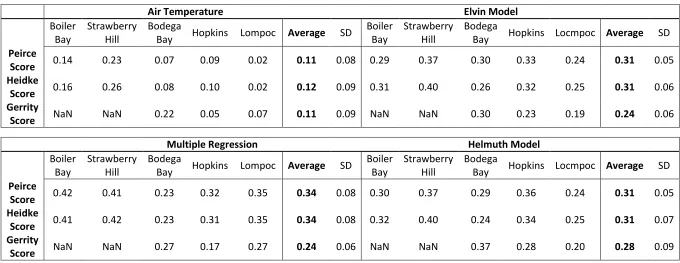
Pierce and Heidke scores for the use of air temperature as a proxy were poor overall; at
Bodega Bay, Hopkins, and Lompoc Landing, they indicated very little improvement in
skill versus a random forecast, although they indicated a slightly larger improvement in
skill at Boiler Bay and Strawberry Hill (Table 1.2). Still, scores for air temperature at the
northern sites were poorer than for other methods at the same locations, strongly
cautioning against the use of air temperature alone as a proxy, especially when heat stress
is of concern. It is also important to note the inter-logger variability in skill scores,
especially considering that each set of observations was taken by instruments separated
27
Pierce, Heidke, and Gerrity scores indicated relatively little difference between
the Helmuth biophysical model, the Elvin model, and the multiple regression approach
(Table 1.2). However, when applied to a physiological framework, each predictive
method demonstrated different levels of skill at different points along the physiological
performance curve, and the temperatures at which each model was most skilled varied
with geographic location. At all sites, hit rates indicated more success (values closer to
1) at low to mid temperatures than at high temperatures, with the highest values being
reported for the 10°-17° C range at most sites (Figure 1.3). On the other hand, false alarm
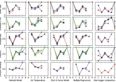
ratios for the lowest temperature category were also high at all sites, indicating the
tendency of all models to “run cold” (Figure 1.4).
Results from the inter-logger analysis indicated almost-perfect hit rates at all sites
for temperatures falling between 10° and 17°C. Overall, hit rates tended to decrease as
temperatures increased at all sites, although at Boiler Bay, Strawberry Hill, and Hopkins,
hit rates for the 22-32°C category were higher than those for 17-22°C. At four sites, hit
rates decreased to 0 for temperatures above 38°C; the notable exception is Strawberry
Hill, for which inter-logger hit rates indicated that loggers were recording similar high
temperatures.
False alarm ratios for the inter-logger analysis varied across categories and across
sites. Due to the nature of forecasts with multiple categories, a “miss” in one category is
a “false alarm” in another. Because of the high variability in maximum temperatures and
small sample sizes for the two highest categories (32-38°C and>38°C), the false alarm
28
for the inter-logger analysis had values closer to 1 (indicating less skill) at high
temperatures, although this trend is not consistent across sites.
At all sites, hit rates for air temperature were highest for the cold suboptimal band
of 10°-17°C; at Bodega Bay and Lompoc Landing, cold suboptimal hit rates exceeded
0.9. However, hit rates for the next highest temperature category (optimal, 17°-22° C)
were quite poor, and virtually no skill was gained by using air temperature as a proxy for
body temperature within the suboptimal high, sublethal high, and lethal high categories.
Results strongly caution against the use of air temperature as a metric for heat stress,
since, at all sites, air temperature greatly under-predicted the number of instances mussels
experienced optimal, high suboptimal, high sublethal, and high lethal temperatures.
Hit rates for the Elvin & Gonor model were generally comparable to or slightly
lower than hit rates for air temperature alone at the cold sublethal and cold suboptimal
levels and indicated more model skill in predicting temperatures at optimal levels.
Although the Elvin and Gonor model was developed for a site near to Strawberry Hill
and Boiler Bay, the hit rate was relatively low for high suboptimal temperatures at these
sites. Hit rates indicated some skill at predicting high suboptimal temperatures at Bodega
Bay and Hopkins.
The skill of multiple regression approaches varied from site to site and from
category to category. At Strawberry Hill, Bodega Bay, and Hopkins, hit rates for
multiple regression approaches were similar to those of the Elvin and Gonor model,
whereas at Lompoc Landing and Boiler Bay, hit rates indicated more skill at predicting
29
Hit rates for the Helmuth biophysical model were generally lower than other
approaches at cold sublethal and cold suboptimal temperatures. The biophysical model
had higher hit rates than other methods for the 22-32°C range at Bodega Bay and
Hopkins.
A common trend among all models were hit rates of 0 and incalculable false
alarm ratios for temperatures greater than 38°C, which indicates that although loggers
reached high temperatures, these conditions were not predicted by the models. Since the
ability to predict extreme conditions is imperative to predicting the potential effects of
30 1.4 DISCUSSION
In light of a changing climate, it is important to be able to predict sublethal levels of
stress as well as lethal conditions, and models designed to make these predictions must
perform well along the entire width of the physiological performance curve. Results from
this study emphasize the importance of evaluating model performance in context of an
organism’s physiology. While statistics such as RMSE indicated that models were
performing relatively well, hit and false alarm rates indicated different levels of
performance within different regions of the performance curve Probability distributions
of body temperature are predicted to be centered slightly below optimal in order to
maximize overall fitness under fluctuating conditions (Martin & Huey, 2008); therefore,
the most ecologically damaging conditions are stressful events and extremes, since
organisms that cannot withstand the harshest conditions that occur at a particular location
will not be able to occupy it (Gaines & Denny, 1993). In light of this, the tendency of
model performance to decrease as organisms experienced higher temperatures is
especially troubling. The fact that, in many cases, hit rates were 0 (and false alarm ratios
incalculable due to division by 0) for the sublethal high and lethal high categories
indicate that these particular models may be unable to predict high temperatures.
It is important to note that all three of the methods I used are based only on one or
two environmental parameters, and that even the biophysical model used in this study
makes a number of simplifying assumptions. More complex biophysical models designed
to predict body temperatures of M. californianus exist (ex. Gilman et al., 2006a; Wethey
et al., 2011b) future work would involve applying this same physiological framework to
31
Should a model be capable of predicting extreme high temperatures, a
physiologically-grounded approach will also elucidate some of the difficulties faced in
predicting and verifying a model’s ability to predict extreme events. Extreme events are
also rare events (Casati et al, 2008; IPCC, 2012) and this rarity leads to small sample
sizes and, as a result, large sampling uncertainties. For example, though several years of
data were pooled at each site in this study, sample sizes of observed temperatures for the
high sublethal and high lethal categories consisted of only a handful of data points.
A second difficulty in predicting extreme events, especially extreme highs, in this
context lies in the variable nature of the intertidal zone itself. In this case, the use of data
from one logger as a forecast for another also indicated low levels of skill at high
temperatures, even though data were collected from microsites with similar wave
exposures and substratum angles, further emphasizing how localized heat stress events
may be. Denny et al. (2011) found that, while the mean range of maximum body
temperatures between individual mussels in a single exposed bed was 3.7°C,
inter-individual variation in body temperature could be as large as 11.7°C. The rocky intertidal
zone is spatially heterogeneous, and factor such as substratum angle strongly influence
the temperatures organisms experience (e.g. Helmuth & Hofmann, 2001; Wethey, 2002).
Furthermore, wave splash modulates patterns of emersion and immersion in intertidal
systems (Gilman et al., 2006b), and predictions generated using the Helmuth biophysical
model were sensitive to changes in estimates of wave run-up (pers. obs). As a result, even
the most skilled models available may not be able to explicitly predict the temperatures
organisms in the field will experience but rather the probability that certain thresholds of
32
Despite the inter-individual variability in predicting high body temperatures and
uncertainty in verifying predictions in this region, this analysis provides some insight into
the methods necessary to gain an understanding of physiological stress in the field. The
ability of air temperature to serve as an effective proxy for body temperature decreases
sharply once body temperatures reach what could be considered “optimal” (17-22°C).
Although a variety of factors influence the thermal regime of rocky-shore organisms,
high temperatures are driven primarily by interactions of air temperature (a climatic
factor) and solar radiation (a non-climatic factor) (Denny & Harley, 2006). Solar
radiation, in particular, has a profound effect on maximum temperatures experienced by
M. californianus (per sobs), reflected in the poor predictive capacity of air temperature in
regards to physiological heat stress. Recent studies have suggested that thermal
adaptation of certain intertidal species may be driven primarily by adaptation to
non-climatic sources of heat (Marshall et al, 2010); however, most studies do not distinguish
between heating from the ambient air and solar heating (Helmuth et al., 2006). Although
climate change will not directly affect the amount of solar irradiance reaching the surface,
a thorough understanding of non-climatic sources of heat and their interaction with
climatic sources will be necessary to gain an understanding of how climate change might
affect intertidal systems.
Surface air temperatures are predicted to increase under future climate scenarios
(IPCC, 2007); in conjunction with high solar radiation, this will likely shift an organism’s
average location along its physiological performance curve to the right. Because of the
left-skewed nature of physiological performance curves, even a slight increase in body
33
lethal temperatures, high suboptimal temperature temperatures are not rare occurrences.
At the two central sites (Bodega Bay and Hopkins), hit rates for the biophysical model for
high suboptimal temperatures were higher than those for other methods, which suggests
some skill of this approach at predicting high temperatures.
Cold stress in M. californianus has typically received less attention than heat
stress. Except for situations when the loss of infrared radiation in high (e.g. clear nights),
air temperature sets the lower limit to body temperature in the absence of evaporative
cooling, and air temperature was shown to be an effective proxy for cold stress when
applied to a winter mortality even in the invasive mussel Perna viridis. (Firth et al.,
2011). Air temperature alone tended to overestimate the number of hourly occurrences
within the coldest temperature bins, likely due to the influence of solar heating during the
day. However, since both minimum air temperature and the most stressful cold
temperatures are likely to take place at night, when the effect of solar insolation is absent,
minimum air temperature may still remain a useful proxy for cold stress.
It is important to note that both cold stress and heat stress events are
time-dependent. While short-term exposures to extremes can result the restructuring of an
ecosystem (Wethey et al., 2011a), sublethal effects can lead to reproductive failures
(Petes et al., 2008) and negative energy balance. In addition, while organisms may be
able to withstand short term exposures to extreme temperatures, more moderate
temperatures may become lethal as the window of exposure is expanded. For example,
while M. californianus was shown to survive short term (8-hour) exposures to extreme
cold temperatures (2°C), as of yet, it is unknown how chronic or long-term exposures to
34
exposures to sublethal temperatures can be as ecologically relevant as short-term extreme
events, any models designed to predict the effects of climate change be able to accurately
reflect sublethal temperatures as well as lethal.
Results also indicate a lack of model stationarity at certain sites, most notably at
Lompoc Landing. Here, recorded temperatures exceeded temperatures predicted by the
biophysical model (Figure 1.4), and in terms of both physiological bins and overall
statistics, the most “skilled” model at higher temperatures was the multiple regression
tailored specifically for that site. The failure of the general models at Lompoc Landing
may indicate gaps in our ability to account for the effect of local topography. Since more
complex biophysical models have been observed to perform well at certain sites and less
well at others (e.g. Gilman et al., 2006a, Wethey et al., 2011), this suggests that a more
thorough understanding of the effect of topography on the interactions between
environment and organism is necessary to apply the assumption of model stationarity to
35
TABLE 1.1 Bias, RMSE, and MAE of all models at all sites
Bias
Bodega Bay Hopkins Lompoc Boiler Bay Strawbery Hill Average SD
Air Temperature -2.93 -3.56 -6.45 -4.83 -4.44 -4.44 1.34
Elvin Model 0.93 -0.34 -2.66 -2.51 -1.02 -1.12 1.51
Multiple Regression -0.91 -0.86 1.41 -1.53 -0.84 -0.55 1.13
Helmuth Model 1.95 0.69 -2.78 -2.21 -0.76 -0.62 1.97
RMSE
Bodega Bay Hopkins Lompoc Boiler Bay Strawberry Hill Average SD
Air Temperature 5.25 6.11 8.83 8.17 5.55 6.78 1.62
Elvin Model 4.20 4.13 5.45 5.90 4.07 4.75 0.86
Multiple Regression 4.29 4.17 4.52 4.80 3.91 4.34 0.34
Helmuth Model 4.73 4.39 5.57 5.88 4.03 4.92 0.78
Mean Absolute Error
Bodega Bay Hopkins Lompoc Boiler Bay Strawberry Hill Average SD
Air Temperature 3.68 4.51 6.88 5.62 3.72 4.88 1.37
Elvin Model 3.26 3.08 3.85 3.96 2.70 3.37 0.53
Multiple Regression 3.08 3.10 3.53 3.31 2.60 3.12 0.34
36
TABLE 1.2 Forecast verification skill scores for all models at all sites
Air Temperature Elvin Model
Boiler Bay
Strawberry Hill
Bodega
Bay Hopkins Lompoc Average SD
Boiler Bay
Strawberry Hill
Bodega
Bay Hopkins Locmpoc Average SD
Peirce
Score 0.14 0.23 0.07 0.09 0.02 0.11 0.08 0.29 0.37 0.30 0.33 0.24 0.31 0.05 Heidke
Score 0.16 0.26 0.08 0.10 0.02 0.12 0.09 0.31 0.40 0.26 0.32 0.25 0.31 0.06 Gerrity
Score NaN NaN 0.22 0.05 0.07 0.11 0.09 NaN NaN 0.30 0.23 0.19 0.24 0.06
Multiple Regression Helmuth Model
Boiler Bay
Strawberry Hill
Bodega
Bay Hopkins Lompoc Average SD
Boiler Bay
Strawberry Hill
Bodega
Bay Hopkins Locmpoc Average SD
Peirce
Score 0.42 0.41 0.23 0.32 0.35 0.34 0.08 0.30 0.37 0.29 0.36 0.24 0.31 0.05 Heidke
Score 0.41 0.42 0.23 0.31 0.35 0.34 0.08 0.32 0.40 0.24 0.34 0.25 0.31 0.07 Gerrity
38
39
40
Figure 1.4 False alarm ratios for all models at all sites. Category labels are as follows: 0 represents temperatures from less than 0°C; 1 represents 0-10°C. 2 represents 10-17°C; 3 represents 17-22°C; 4 represents 22-32°C; 5 represents 32-38°C; and 6 represents 38°
41
CONCLUSION
In light of a changing climate, it is essential that any model used to predict the
thermal conditions an organism experiences performs well for the prediction of extreme
events as well as mean conditions. In my thesis, I applied forecast verification metrics
commonly used to analyze meteorological models to several simple and biophysical
ecological models. I also applied a physiological framework to the predictions made by
the models, to assess model performance based on levels of physiological stress the
organisms experienced.
While all models performed relatively well at low temperatures, model
performance decreased as temperatures rose. Variability in body temperatures of
individual mussels also increases as temperatures increase; however, none of the models
were capable of predicting extreme high temperatures. This poor performance was not
reflected in commonly used methods of measuring model skill, such as RMSE. Since
both sublethal stressors and extreme conditions affect an organism’s survival and fitness
(Petes et al. 2008; Jones et al. 2009, 2010; Sorte et al. 2011), the models’ lack of ability
to predict these conditions is troubling and limits their use for the purpose of predicting
the effects of climate change. My thesis emphasizes the need to match tests of model
skill with physiologically meaningful metrics to ensure that the models use for the
42
REFERENCES
Bayne, B.L., Bayne, C.J., Carefoot, T.C., et al. The physiological ecology of Mytilus californianus Conrad. Oecologia. 22. 211-228.
Buckley, L.B., Urban, M.C., Angilletta, M.J. et al. (2010). Can mechanism inform species distribution models? Ecology Letters. 13: 1041-1054.
Casati, B., Wilson, L.J., Stephenson, D.B. et al. (2008). Forecast verification: current status and future directions. Meteorological Applications. 15:1. 3-18.
Chapperon, C., Seuront, L. (2011). Behavioral thermoregulation in a tropical gastropod: links to climate change scenarios. Global Change Biology. 17. 1740-1749.
Denny, M.W., Harley, C.D.G. (2006). Hot limpets: predicting body temperature in a conductance-mediated thermal system. Journal of Experimental Biology. 2409-2419.
Denny, M.W., Hunt, L.J.H., Miller, L.P. et al. (2009). On the prediction of extreme ecological events. Ecological Monographs. 79:3. 397-421
Denny, M.W., Dowd, W.W., Bilir, L., et al. (2011). Spreading the risk: Small-scale variation among intertidal organisms and its implications for species persistence. Journal of Experimental Marine Biology and Ecology. 400. 175-190.
Elvin, D.W., Gonor, J.J. (1979). Thermal regime of an intertidal Mytilus californianus conrad population on the central Oregon coast. Journal of Experimental Marine Biology and Ecology. 39. 265-279.
Etter, R.J. (1988). Physiological stress and color polymorphism in the intertidal snail Nucella lapillus. Evolution. 42:4. 660-680.
Firth, L.B., Knights, A.M., Bell, S.S. (2011). Air temperature and winter mortality: Implications for the persistence of the invasive mussel Perna viridis in the intertidal zone of the south-eastern United States. Journal of Experimental Marine Biology and Ecology. 400. 250-256.
Fitzhenry, T., Halpin, P.M., Helmuth, B. (2004). Testing the effects of wave exposure, site, and behavior on intertidal mussel body temperatures: applications and limits of temperature logger design. Marine Biology. 145: 339-349.
Gaines, S.D., Denny, M.W. (1993). The largest, smallest, highest, lowest, longest, and shortest- extremes in ecology. Ecology. 74:6. 1677-1692.
43
Gilman, S.E., Wethey, D.S., Helmuth, B. (2006). Variation in the sensitivity of
organismal body temperature to climate change over local and geographic scales. Proceedings of the National Academy of Sciences. 103:25. 9560-9565.
Gilman, S.E., Harley, C.D.G., Strickland, D.C. et al. (2006). Evaluation of effective shore level as a method of characterizing intertidal wave exposure regimes. Limnology and Oceanography: Methods. 4. 448-457.
Hawkes, L.A., Broderick, A.C., Godfrey, M.H. et al. (2007). Investigating the potential impacts of climate change on a marine turtle population. Global Change Biology. 13. 923-932.
Helmuth, B. (1998). Intertidal mussel microclimates: predicting the body temperature of a sessile invertebrate. Ecological Monographs. 68:1. 51-74
Helmuth, B. (1999). Thermal biology of rocky intertidal mussels: quantifying body temperatures using climatological data. Ecology. 80:1. 15-34
Helmuth, B., Hofmann, G.E. (2001). Microhabitats, thermal heterogeneity, and patterns of physiological stress in the rocky intertidal zone. Biological Bulletin. 201. 374-384.
Helmuth, B. (2002). How do we measure the environment? Linking intertidal thermal physiology and ecology through biophysics. Integrative and Comparative Biology. 42. 837-845.
Helmuth, B., Yamane, L., Lalwani, S., et al. (2011). Hidden signals of climate change in intertidal ecosystems: What (not) to expect when you are expecting. Journal of Experimental Marine Biology and Ecology. 400. 191-199.
Huey, R.B., Kingsolver, J.G. (2011). Variation in universal temperature dependence of biological rates. Proceedings of the National Academy of Sciences. 108:26. 10377-10378.
Huey, R.B., Stevenson, R.D (1979). Integrating thermal physiology and ecology of ectotherms-discussion of approaches. American Zoologist. 19:1. 357-366.
Hutchinson, G.E. (1957). Concluding Remarks, Cold Spring Harbor Symposium, Quantitative Biology. 22: 415-427